Article

Multi-Objective Optimized Aggregation of Demand Side Resources Based on a Self-organizing Map Clustering Algorithm Considering a Multi-Scenario Technique

1
School of Electrical and Electronic Engineering, North China Electric Power University, Baoding 071003, China
2
College of Electrical Engineering, Zhejiang University, Hangzhou 310027, China
*
Authors to whom correspondence should be addressed.
Energies 2017, 10(12), 2144; https://doi.org/10.3390/en10122144
Submission received: 9 November 2017 / Revised: 29 November 2017 / Accepted: 6 December 2017 / Published: 15 December 2017

Abstract

:
To fully investigate the characteristics and the complementarities of demand side resources (DSRs), and to achieve efficient utilization of resources, the aggregation of DSRs is studied in this paper. Considering the uncertainty of DSRs, the characteristics analysis and the selection of relevant daily feature corresponding to various types of DSR are carried out. Then a multi-scenario model based on quarter division and self-organizing map (SOM) neural network algorithm is proposed. In the model, the clustering feature vector is selected as the input vector of the SOM algorithm to perform DSR clustering analysis to get the different scenarios. In addition, to obtain the resource aggregation (RA) with good load characteristics, response characteristics and distributed generation (DG) consumption, a multi-scenario objective optimization aggregation model of DSR based on scenario partition is established, and an the model is solved by an improved niche evolutionary multi-objective immune algorithm. Finally, the case studies are given to verify the validity of the model.

1. Introduction

The active distribution network (ADN) concept provides a new solution for the access and consumption of distributed energy resources (DERs) and the efficient utilization of distribution network (DN) resources [1,2,3]. In this paper, the resources with enormous quantities and various different features in ADN are collectively referred to as the demand side resources (DSRs). Currently, for the study of the resource utilization, how to fully extract the characteristics and complementarities of various DSRs and achieve efficient utilization of resources has become a hot issue in the resource utilization research area [4]. However, due to the features of DSRs, with dispersed distribution, various kinds and different features, it is difficult for a single DSR to directly participate in the electricity market transaction, so aggregation technology is widely used [5]. Aggregation refers to the integration of a large number of dispersed resources into a polymer with large scheduling capacity, good regulation characteristics and simple regulation according to the external environment or the operation purpose, which is an important means for distributed resources management and coordination. Lots of studies have been done for the resource aggregation [6,7,8,9,10,11,12,13]. In [6], considering the complementarity of DERs, the landscape theory is taken to aggregate a multi-microgrid (MG). Through the aggregation, the different MGs can help each other, which may effectively reduce the impact of the uncertainty of MG output power, and increase the individual economic benefit and enhance the security of power system. In [7], an electric vehicle (EV) aggregation method based on the load aggregator (LA) idea is proposed, in which the dispersed EV energy storage resources are effectively aggregated with the uncertainty of EV behavior features taken into account. In [8], based on the device level simulation DSR evaluation mechanism and the DSR quality division standard, the DSR aggregation model with multi-user load group is proposed. In [9], the virtual power plant (VPP) is employed to aggregate the large amount of wind power and EV in the integration system. With the goal of maximizing the comprehensive income of VPP and EV discharge, the optimal model of power generation plan is established under the constraints of power balance. In [10], the controllable air conditioner load is composed of VPPs, and the optimization model in which the maximize load reduction in VPPs is taken as the objective is established to determine the load reduction during each period.
Through the analysis of the existing literature, it can be found that the research of the DSR aggregation is relatively abundant. In some literatures, the same kind of DSR is aggregated to improve the DSR scale and capacity, and in others the complementary features and capacity of different kinds DSR are considered to aggregate them into LA, MG or VPP. The aggregation schemes are usually aimed at the single aggregation under the typical scenarios of long time scale, and less consideration is given to the uncertainty in the system operation. However, the existence of the uncertainty of DSR is inevitable, and some of the effects for the system operation cannot be ignored [14].
Considering that the DG represented by wind turbines (WTs) and photovoltaic (PV), residential loads and commercial loads are easily affected by meteorological factors and show certain seasonal differences. In this paper, a separate season aggregation thought is introduced for a certain area of DSR, and the existing uncertainty of daily DG output and daily load fluctuation in each season aggregation are considered. The Monte Carlo method is used to solve the probability models of uncertainty in [15,16]. In [17,18,19], Latin hypercube sampling and sample reduction technology are used to deal with the uncertainty of DG output and load fluctuation, and the construction of the multiple scenarios is carried out. In [20], The K-means clustering and multi-scenario probability analysis is adopted to reduce the effect of uncertainty on the DG output and load fluctuation. Therefore, on the basis of the above research, the characteristics analysis and the selection of relevant daily feature corresponding to various types of DSR are carried out, and the DSR clustering feature vector is selected as the input vector of SOM algorithm to perform DSR clustering analysis to get the different scenarios [21]. Then, the multi-objective optimization aggregation model of DSR in single season is established based on the scenario partition. Finally, a practical case study is employed to verify the validity and effectiveness of the method proposed in this paper.

2. Multiple Scenarios Construction of DSR Aggregation

2.1. Demand Side Resource Characteristics Analysis and Features Quantities Extraction

2.1.1. Demand Side Resource Introduction

ADN contains many types of resources, including load resources and distributed generation resources. In this paper, all resources are defined as DSR in ADN. The DSR include inflexible loads, flexible loads, distributed generation, electric vehicles and energy storage, which are located on the user side and closely linked with users. The DSR also have the characteristics of dispersed distribution, widely variety, different features, and so on. Figure 1 shows a detailed composition of the DSR.

2.1.2. The Timing Characteristics Analysis and Daily Features Quantities Extraction of DG Output and Load Fluctuation

DG (taking WT and PV as example in this paper) output has obvious seasonality due to the different wind speed and light intensity in different seasons, but it is not accurate enough to artificially take each season of a year as a scenario (each scenario lasts for three months) based on experience alone. Considering the obvious daily periodicity of DG output, representative daily feature quantities can be selected, and the clustering method is used to cluster the daily output curve in each season and refine the rough scenarios. The daily average value, the daily maximum value and the daily peak valley difference value of DG output are selected as the features quantities of DG generation in this paper. Similarly, the demand side load also has obvious daily periodicity. In order to distinguish the seasonal and holiday characteristics of load fluctuations, the daily average value, the daily maximum value and the daily peak valley difference value of daily load curve are selected as the features quantities of the load characteristic curve.

2.1.3. The Response Characteristics and Features Quantities Extraction of the Demand Response Resources

DSR contains a lot of demand response resources (DRRs), including flexible loads, EV charging loads, etc., and the response characteristics of the same response resource are uncertain in different periods. For example, a user’s daily response capacity, response speed, and default power will be different under different power consumption conditions. However, users with different response capabilities will receive different levels of reward and punishment. It is unfair to apply a single policy of reward and punishment to a user in different scenarios. It will also lead to irrationality of response resource regulation in the long term. Therefore, it is necessary to divide the scenarios according to the differences of response capability of the demand response resources.
DRRs mainly include transferable load (TL) and interruptible load (IL), which have different response characteristics in them. In the assessment of response capability, firstly, the response potentials of different response type resource are respectively analyzed based on different load characteristics. Then, a response aggregation model of multi-type response resources is constructed to represent the response capabilities of user response resources.
(1) The response characteristic and mathematical model of TL
TL is flexible in power consumption, and the total power consumption required for the completion of the work is certain, and it has the ability of load transfer. This type of equipment is represented by ATL and its electrical characteristic is described as follows:
V a = [ p a min , p a max , t a s t a r t , t a e n d , Q a min ] ,    a A T L
where, Va is the load characteristic; p a min and p a max are the minimum power consumption and the maximum power consumption of equipment a; t a s t a r t and t a e n d are the starting run time and the ending run time of equipment a; Q a min is the minimum power consumption to complete task.
Based on the Equation (1), the power consumption of TL in time t is described as (2):
{ p a min p a t p a max , t [ t a s t a r t , t a e n d ] p a t = 0 , t [ t a s t a r t , t a e n d ] Q a min p a t , t [ t a s t a r t , t a e n d ]
It can be known from Equation (2) that the power is in the allowable range during the operation period of TL and the power consumption should meet the minimum power consumption requirement at the end of the operation. TL can participate in load dispatching response to power grid demand by transferring electrical time period and guaranteeing completion of work requirements.
(2) The response characteristic and mathematical model of IL
The power consumption of IL can be interrupted at any time, but its working state will change. The power consumption will be reduced by the interruption of the load. The interruption time of IL is usually limited by the user comfort. This type of equipment is represented by AIL and its electrical characteristic is given by Equation (3):
V a = [ p a min , p a max , t a s t a r t , t a e n d , θ a min ] ,    a A I L
where, θ a min is the minimum comfort requirement that the equipment a needs to meet.
Then the power consumption of IL in time t is defined as:
{ 0 p a t p a max , t [ t a s t a r t , t a e n d ]    and    θ a t > θ a min p a min p a t p a max , t [ t a s t a r t , t a e n d ]    and    θ a t θ a min p a t = 0 , t [ t a s t a r t , t a e n d ]
where, θ a t is the user’s actual comfort value in time t.
During the operation of IL, the minimum power consumption can be 0 when the equipment actual state meets the user's comfort requirement. IL can participate in load dispatching to meet grid requirements within user comfort levels.
After analyzing the response potential of different types response resources, the ladder aggregation model proposed in [22] is adopted to obtain the users response capacity, and the response characteristics including the daily response capacity and response time are received. In addition, the user cannot respond to the contract completely when they participate in the demand response. The difference between the actual response capacity and the contract capacity is defined as the default power. The default power is also an important index to reflect the user response capability. So, the daily response capacity, response time, and default power of the response resource are selected as the characteristic quantities of the response characteristic of the demand response resource based on the load power statistics characteristic in this paper.

2.1.4. The Constitution of Clustering Analysis Features Quantities

Based on the above introduction of DSR characteristics analysis and daily related features quantities extraction, the clustering features quantities X is represented by Equation (5) when DSR that participate in aggregation in a certain region is used for aggregation analysis:
X = ( x 1 1 , x 2 1 x m 1 , x 1 2 , x 2 2 x n 2 , x 1 3 , x 2 3 x q 3 )
where, x m 1 is the daily output feature vectors of the mth DG (defined as the first class DSR), x m 1 = ( x m , 1 1 , x m , 2 1 , x m , 3 1 ), x m , 1 1 , x m , 2 1 , x m , 3 1 represent the daily average value, the daily maximum value and the daily peak valley difference value of the mth DG output, respectively; x n 2 is the daily load feature vectors of the nth inflexible load (defined as the second class DSR) which participate in the aggregation, x n 2 = ( x n , 1 2 , x n , 2 2 , x n , 3 2 ), among them, x n , 1 2 , x n , 2 2 , x n , 3 2 represent the daily average value, the daily maximum value and the daily peak valley difference value of the nth inflexible load respectively; x q 3 is the daily output feature vectors of the qth demand response load (defined as the third class DSR, including flexible load and electric vehicle charge load); x q 3 = ( x q , 1 3 , x q , 2 3 , x q , 3 3 , x q , 4 3 , x n , 5 3 , x n , 6 3 ), among them, x q , 1 3 , x q , 2 3 , x q , 3 3 , x q , 4 3 , x n , 5 3 , x n , 6 3 represent the daily average value, the daily maximum value, the daily peak valley difference value of , the daily response capacity, response time and default power of the qth demand response load, respectively.

2.2. The Multiple Scenarios Building Based on Quarterly Division and SOM Algorithm

2.2.1. DSR Quarterly Analysis

The DG represented by WT and PV, whose output is greatly influenced by meteorological factors, and meteorological factors show different patterns with the changes of the seasons, so the DG output has obvious seasonality. In [23], a functional nonparametric regression model is established, which uses historical output data of a wind farm in recent years to predict the typical daily curves of the WT output under four seasons. This is shown in Figure 2a. Similarly, the typical daily curve of the PV power is obtained by using the historical output data of a photovoltaic power station in recent years, which is shown in Figure 2b.
It can be known from Figure 2 that WT and PV power are basically below the rated power, and WT is decreasing in the order of winter, spring, autumn and summer; the PV power is decreasing in the order of summer, spring, autumn and winter.
For residential loads and commercial loads (taking the north user as an example), the residential load is commonly a type of peak facing load, and there are two peak periods of electricity consumption: the morning peak and the evening peak. For commercial loads, during the business day, the load value is obviously increased. There is a constant peak load during daytime and a valley load period at night. In addition, due to the existence of summer air conditioning loads and winter heating equipment use, the load values in summer and winter are higher than the load values in spring and autumn. Therefore, there are also obvious seasonal differences in the residential and commercial loads. The typical daily curves of the residential load and commercial load are shown in Figure 3.
According to the above analysis, the aggregation of DSR is divided into four typical quarters considering all kinds of DSR seasonal differences in this paper. For each quarter, the SOM algorithm is used to cluster analysis according to the daily characteristics of aggregated resources, and several subdivision scenarios and their probability of occurrence are obtained. In the subsequent chapters, the existence of multiple scenarios will be fully considered in the multi-types resource optimization selection to get an optimal aggregation solution which satisfies the multi-scenarios situation, makes the aggregation of resources more reasonable and gives full play to the features of multi-type resources and the complementarity between them.

2.2.2. SOM Algorithm

The SOM neural network is an unsupervised and competitive learning network. It can identify environmental features and cluster them automatically. It is widely used in load clustering analysis [21,24]. The SOM neural network consists of two layers (an input layer and an output layer). Through the variable weights each input layer neuron is connected to the output layer neuron, and the output neuron forms a two-dimensional planar array.
In this paper, the feature vector X, which is composed of various DSR features, is trained as the input vector of the SOM neural network, and its topological structure is shown in Figure 4.
The training steps are described as follows:
(1)
Confirm the neural network structure. The number of neurons in the input layer is i = 3m + 3n + 6q (the dimension of the vector X), each neuron corresponds to a component of the input vector, and the output neuron number is j = J.
(2)
Initialization. The connection weight wij(t) of the input layer neuron to the output layer neuron is given a random values between [0,1] intervals.
(3)
The feature vector X, which is composed of various DSR features, is provided to the input layer of the network and deals with it normalized:
X ¯ = X X = ( x 1 1 , x 2 1 x m 1 , x 1 2 , x 2 2 x n 2 , x 1 3 , x 2 3 x q 3 ) ( x 1 1 ) 2 + ( x m 1 ) 2 + ( x 1 2 ) 2 ( x n 2 ) 2 + ( x 1 3 ) 2 + ( x q 3 ) 2
(4)
Calculate the Euclidean distance. Among them, the neuron j* with minimum Euclidean distance is the winning neuron:
d j = i = 1 3 m + 3 n + 6 q ( x i ¯ w i j ) 2 , j = 1 , 2 , , J
(5)
Adjust connection weight vector. Updated the connection weight vector of neurons of j* and its neighborhood Nj*(t):
{ w i j ( t + 1 ) = w i j ( t ) + η ( t ) [ x i ( t ) ¯ w i j ( t ) ] , j = 1 , 2 , , J 0 < η ( t ) < 1
where η(t) is variable learning speed; j* and neighborhood Nj*(t) are decreased along with time.
(6)
Select the feature vector of the new day of aggregation DSR, repeat the learning process from step 3, and until complete the daily feature samples training of each quarter.
(7)
At the end of training, the same output number of neuron represent the class with similarity feature which can be divided into the same class and record the number of days of each category. Taking each category as a segmentation scenario, the probability of occurrence of the scenario is determined by Equation (9).
p s = n s / i = 1 K n i
where K is the number of categories after clustering, and the number of each category is n1, n2, …, ns, …, nK; ps is the probability of the s scenario.
(8)
Obtain the clustering centers of each cluster DSR feature quantities and take it as the features quantities of DSR in each scenario.
It should be emphasized that in the training process of SOM, the difference of network structure, size and training times of the output layer make the training results different. The relative quantization error index Qe and topological error index Te are introduced to represent the quality of SOM clustering [25] to achieve better clustering results. Otherwise, the minimum Davies-Bouldwin Index (DBI) [26] can be selected automatically as the final classification for the display of SOM clustering results.
According to the above analysis, the flow chart of DSR multiple scenarios building based on quarterly division and SOM algorithm is shown in Figure 5.

3. The Multi-Scenario Optimized Aggregation Model of DSR

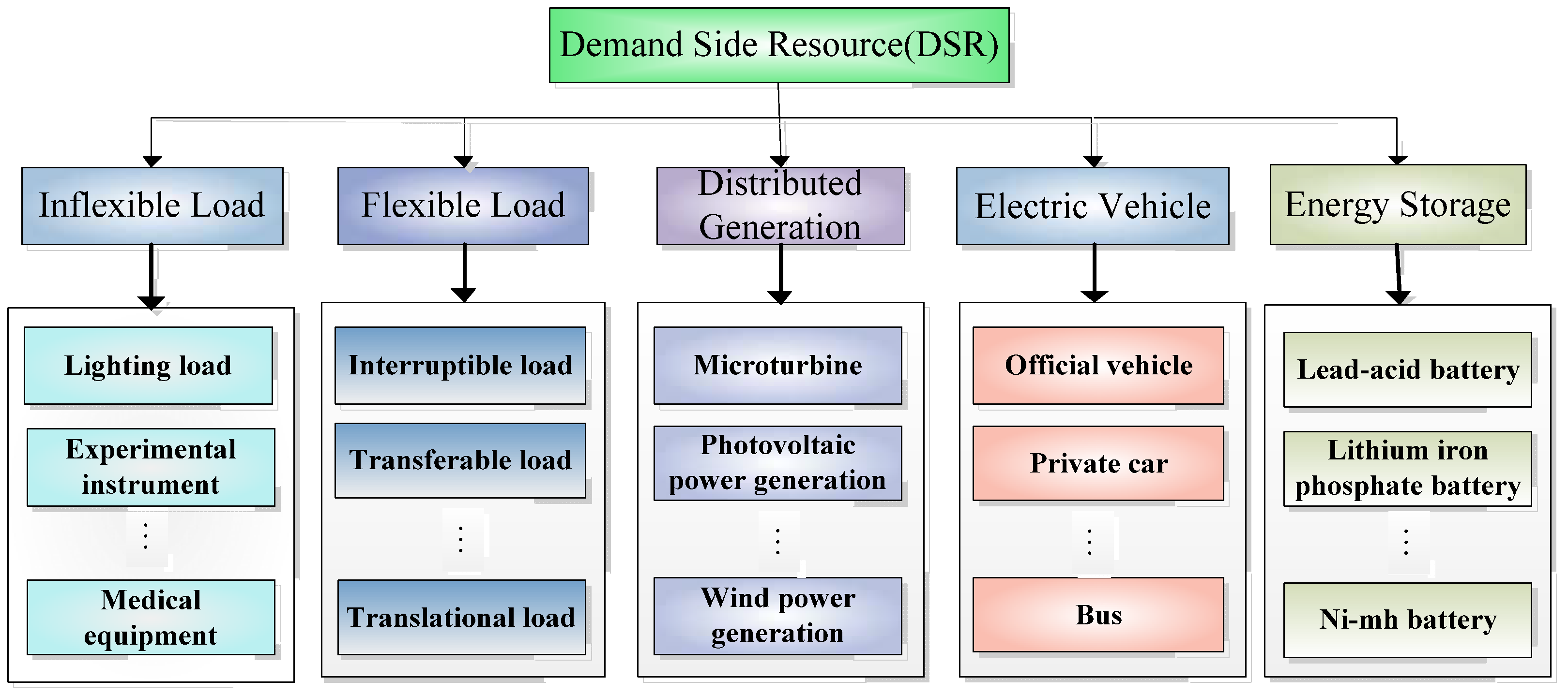
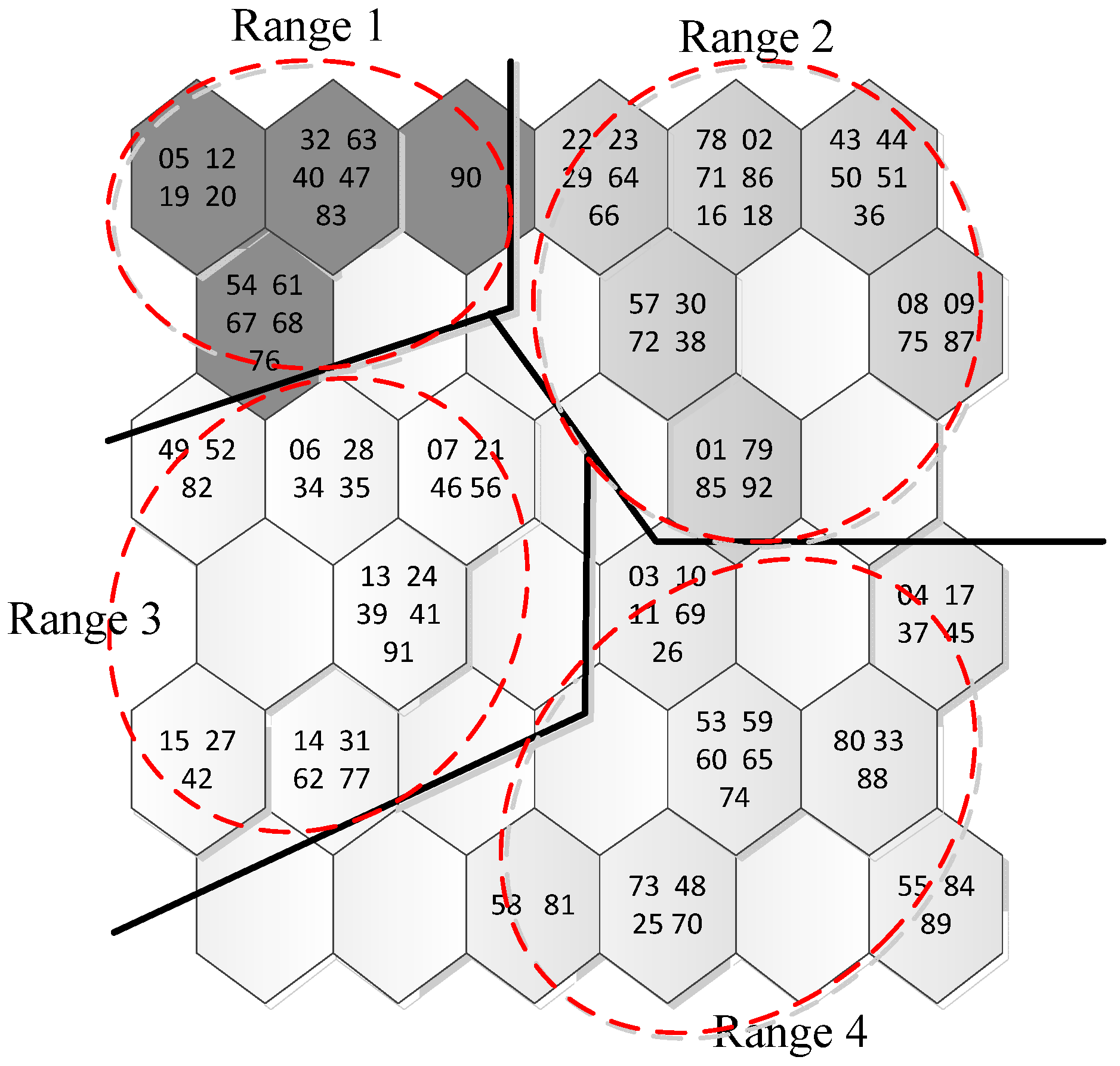
In order to give play to the characteristics of all kinds of DSR and their complementarity, and to fully exploit the response characteristics of the response resources, in the case of ensuring that the interests of users participating in the aggregation are not compromised, many scattered, small capacity and different characteristics DSR are aggregated by multi-objective optimization to form a Resource Aggregation (RA) with good load and response characteristics, to realize the efficient utilization of resources and promote the accommodation of DG, but the aggregation of resources requires a certain amount of time, real-time aggregation is unrealistic and it is not easy to achieve, so this paper takes a quarter as a time measure, aggregates separately in each quarter, and fully considers the existence of multi-scenario in the same quarter. This aggregation thought considers not only DSR temporal difference, but also the influence of non-temporal uncertainty. For example, the responsive uncertainty of response resource, the fluctuation of DG daily output force caused by the change of weather and so on. Otherwise, for certain aggregation areas, the rationality of the number of RA should also be taken into consideration, different locations of different participating users should be considered and the principle of nearby aggregation is adopted. Therefore, this paper makes a simplified treatment, regulates that in a certain area, select the suitable object, and construct an RA. Based on the above analysis, in this chapter, a single-quarter DSR optimized aggregation model is established for a specific region.

3.1. Objective Functions

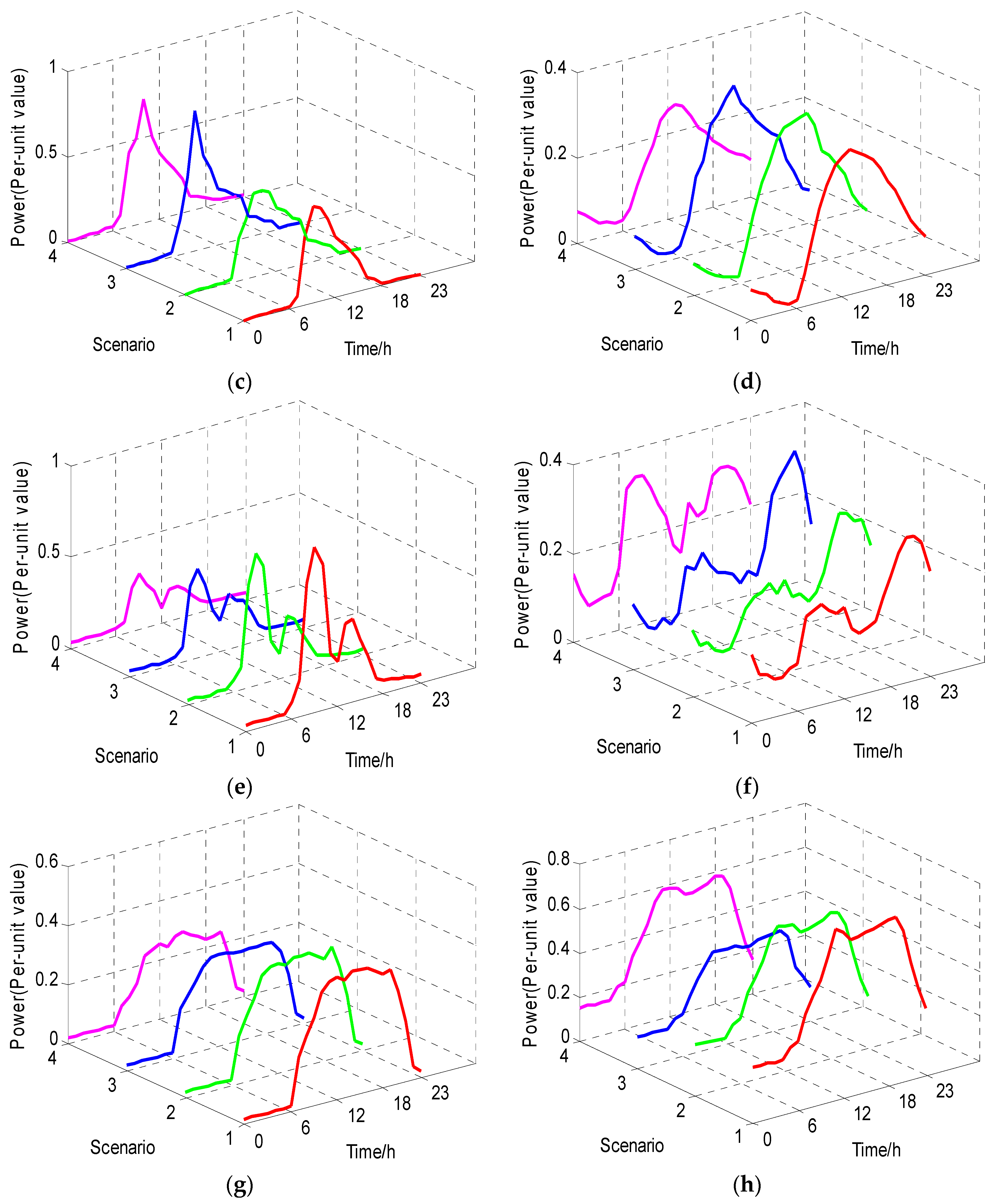
In order to get the optimal construction of the quarterly RA, it needs to take into account the probability of the existence and the appearance of the multi-scenarios. Taking the probability of the scenario as the weight of the single scenario optimization target, the weighted target function of quarterly aggregation is obtained.
(1) Optimal RA load characteristics
(a) The smallest of RA daily peak valley difference:
{ min f 1 = s = 1 K p s [ L o a d max R A ( s ) L o a d min R A ( s ) ] L o a d R A ( s ) = a = 1 m P a t D G ( s ) λ a + b = 1 n L b t l o a d ( s ) λ b + c = 1 q L c t D R ( s ) λ c
where LoadRA(s) represents the daily load curve of the RA in the sth scenario, which the L o a d max R A (s) and L o a d min R A (s) represent the maximum and minimum values of the daily load curve respectively; T = 24, it represents the 24 moments of the load curve; P D G a t (s) is active power of the ath DG in the scenario s at time t; L b t l o a d (s) is the load power of inflexible load b at time t in scenario s; L c t D R is the load power of flexible load c at time t in scenario s; λa, λb, λc are variables, which value are 0 or 1, they represent whether the ath user in the first class DSR, the bth user in the second class DSR and the cth user in the third class DSR participates in the aggregation, respectively. If the value is 1, then it participates in the aggregation and if the value is 0, it does not participate in the aggregation.
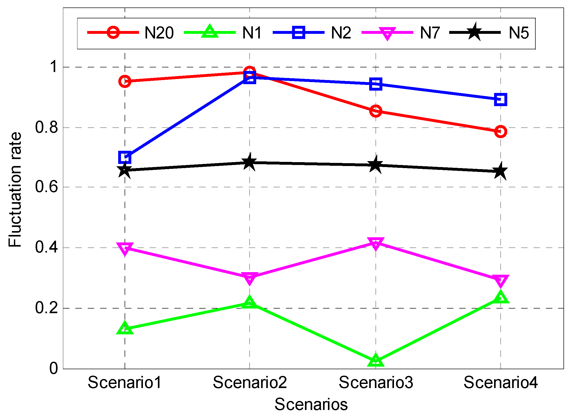
(b) The minimum average daily load volatility of RA
The load fluctuation rate is defined as the ratio of the standard deviation of the load active power σ to the geometric mean μ of the load active power. The geometric mean of load active power σ reflects the level and concentration of the load active power, the standard deviation μ reflects the degree of dispersion of the load active power, and the ratio of the standard deviation of the load active power to the geometric mean reflects the relative size of the load dispersion [27]:
{ min f 2 = s = 1 K ( p s · σ s μ s ) σ s = 1 T t = 1 T ( L o a d t R A ( s ) α s ) 2 μ s = L o a d 1 R A ( s ) · L o a d 2 R A ( s ) · · L o a d T R A ( s ) T
where, σs, μs, αs are the standard deviation, geometric mean and arithmetic mean of the RA load active power in the Scenario s. L o a d t R A (s) is the active power value of the RA load at time t in the Scenario s.
(2) Optimal response characteristics of RA
(a) The largest daily response capacity of RA:
max f 3 = s = 1 K ( p s · c = 1 q Q D R c ( s ) · λ c )
where, Q D R c (s) is the daily response capacity of the response load c in the scenario s.
(b) The lowest RA average daily response cost
In order to encourage the demand response resources to participate in response actively, and to restrain the response user’s default situation of power utilization, we adopt the policy of reward and punishment. First, the resource level (RL) and penalty level (PL) of users are divided according to the response capacity, response time and the default power of different users in a certain scenario, different compensation measure and penalty price are adopted for different resource levels and penalty levels, the classification of different grades for response resources is shown in Table 1.
This paper analyzes the response cost of resources from the perspective of simplified calculation and defines the response cost as the difference between the cost of compensation and the penalty cost to get the target function with the lowest response cost as follows:
min f 4 = s = 1 K ( p s c = 1 q λ c ( Q D R c ( s ) · c i Q b r e c ( s ) · p i ) )
where, Q b r e c (s) is the daily default power of the response load c in Scenario s; ci (i = 1, 2, 3) is the compensation price for the resource level 1, 2, 3 respectively (electricity price of the additional compensation for unit response power); pi (i = 1, 2, 3) is the penalty price of penalty level 1, 2, 3 respectively (electricity price of extra penalty for unit default power).
(c) The highest acceptance level of DG in RA
Promoting distributed power acceptance, reducing the curtailment of WT and photovoltaic, making full use of clean energy, reducing the power of traditional thermal power units and achieving energy conservation and emissions reduction effects are of important significance in the construction of resource aggregation scenarios. When RA is constructed, the supply of load power should be given priority to the supply of distributed energy within the aggregates, and the optimization target is shown in Equation (10):
min f 5 = s = 1 K ( p s t = 1 T ( b = 1 n L b t l o a d ( s ) λ b + c = 1 q L c t D R ( s ) λ c a = 1 m P a t D G ( s ) λ a ) )
In summary, the total objective function of DSR multi-scenario aggregation is:
min F = min ( f 1 , f 2 , 1 f 3 , f 4 , f 5 )

3.2. Constraint Conditions

(1) RA scale constraints
The building of RA is to integrate scattered demand side resources, a large number of small and single dispersed resources. It can be aggregated into an aggregator which has a large capacity and considerable response ability to participate in market operation, facilitating unified dispatching of the market. Therefore, the total number of all types of DSRs involved in aggregation is not too small, and the power consumption after the aggregation is not too small:
{ a = 1 m λ a + b = 1 n λ b + c = 1 q λ c N min ( i ) s = 1 K p s t = 1 T ( b = 1 n L b t l o a d ( s ) λ b + c = 1 q L c t D R ( s ) λ c ) Q RA min = ξ Q Σ
where, Nmin(i)(i = 1, 2, 3, 4) is the lower limit of the number of DSR in the construction of RA in the ith season; Q RA min is the minimum load power of the aggregator after the RA constructed; Q is the total electricity consumption of all users; ξ is a percentage coefficient.
(2) Load complementarity constraints.
In the process of resource aggregation, the complementarity between different loads needs to be fully utilized to reduce the impact of the post-polymerization RA on the system and to improve the stability of system operation [28].
The measurement of load complementarity is the measure of the difference between different load curves at the same time. In other words, the difference between the load curves corresponds to the similarity between the load curves. The higher the similarity between curves, the lower the complementarity. In this paper, the complementarity between loads is measured by the load complement coefficient γ which proposes in literature [28]:
γ y z = 1 β y z
where β is the weighted correlation function at each time between the two load sequences y(t) and z(t) which calculates according to the Equation (18):
β y z = [ t = 1 T Λ ( t ) ( 1 + | Δ y ( t ) / σ y Δ z ( t ) / σ z ) ] / t = 1 T Λ ( t )
where, Λ(t) ≥ 0 is the weight function of active power at different moments according to different degree of importance at different points in time; σy, σz are the standard deviation of load sequence y(t) and z(t), respectively.
In this paper, the sum of the complementary coefficients of the two different user loads in RA is used as the complementarity of the whole aggregator load, as shown in Equation (19):
γ RA = i = 1 m + n + q j = 1 m + n + q γ i j λ i λ j ,    if    i = j , γ i j = 0
where γRA is the measurement of load complementarity between users after the RA is constructed; γij is the load complementarity coefficient between the user i and the user j; λi is the variable that indicates whether the user i participates in the aggregation, the value can be 0 or 1, and if it is 1, the user participates in the aggregation.
In order to ensure the complementarity of the internal load of RA, the following constraint is given, where γmin is the lower limit of load complementarity:
γ RA γ min

3.3. Model Solution

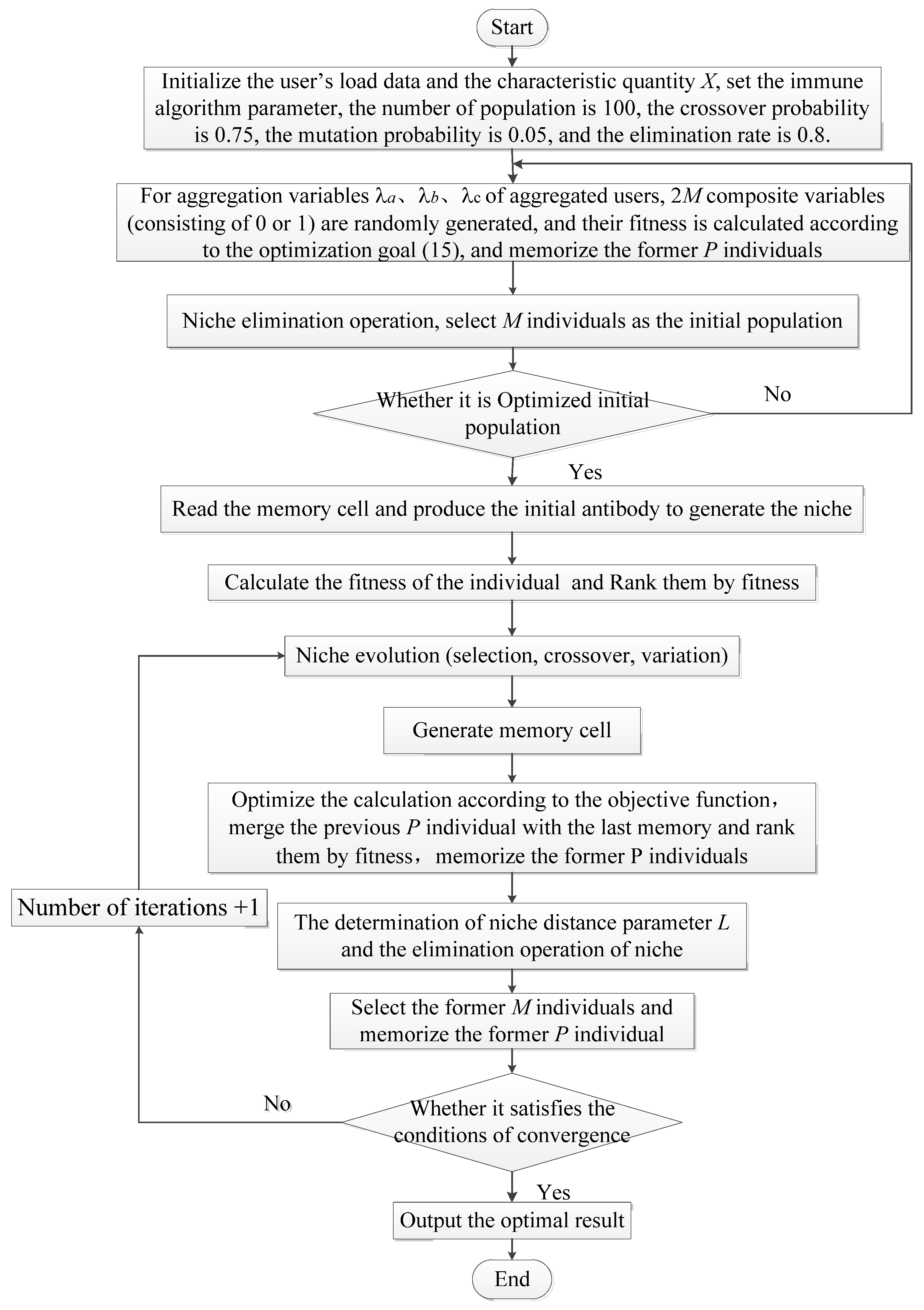
In this paper, the multi-objective immune algorithm for dynamic niche evolution based on niche technique is employed to solve the multi-objective optimization aggregation model of DSR, and the DSR aggregation scheme that meets multiple optimization targets can be obtained from [29].
The basic idea of niche is that in the process of optimization of a multivariate multi-peak function, the solution space is divided into multiple niches and then similar individuals are evolved in specific niches to reach the peak in the habitats. Finally, the optimal solution is obtained among the peaks of the whole habitats. The niche genetic algorithm can effectively improve the efficiency of traditional genetic algorithm optimization; and avoid falling into a local optimal solution. Niche multi-objective immune evolution is a kind of algorithm based on the principle of immune response. The main idea is to use the multi-objective function of the problem to be solved as the antigen of the intrusion immune system, the feasible solution of the multi-objective function as the antibody produced by the immune system, and the affinity of antibodies and antigens (fitness) is used to describe the degree of approximation of the feasible solution and the optimal solution [29].
The affinity of antibodies mainly consists of two aspects: affinity between antibodies, i.e., the similarity, and the affinity of antibodies and the antigens, i.e. the fitness. The similarity of the antibody can be described by the Euclidean distance between the antibodies. If the ith feasible solution is Xi, and the jth feasible solution is Xj, then the ||XiXj|| is the Euclidean distance between Xi and Xj. It is based on the exclusion mechanism to exclude similar individuals in the process of evolution and to maintain the diversity of feasible solutions; therefore more solutions can be searched. The fitness of antibody to antigen can be represented by the reciprocal of the objective function shown in Equation (15). The smaller the objective function value of the antibody is, the closer it is to the optimal solution, and the higher the fitness is. For antibodies with a distance less than a certain value of L, the size of the fitness A(Xi) and A(Xj) is compared. If A(Xi) > A(Xj), a strong penalty function is applied to A(Xj), which makes its fitness become very small. In later evolution, Xj will be eliminated with great probability. The main process of the multi-objective immune algorithm is shown in Figure 6:

4. Example Analysis

4.1. Multi-Scenario Construction and Analysis

In this paper, the power supply range of a city center is taken as an aggregation area, and the summer is taken as an example to analyze. All types of DSR that can be involved in the aggregation area and basic profiles are shown in Table 2.
The users in Table 2 are numbered successively, such as N1, N2, …, N20, which represent the first user in first class DSR, the second user in first class DSR, …, the ninth user in third class DSR respectively. According to the acquired daily output and daily load data on the 20 aggregation users of the summer 92 days, the daily clustering features quantities X on the 20 aggregation users of the summer 92 days can be obtained. The multi-scenario building method based on quarterly division in former contents is adopted in clustering analysis. The input neuron number is i = 4 × 3 + 7 × 3 + 9 × 6 = 87, the output neuron number is j = 6 × 6 = 36, and the clustering results are shown in Figure 7.
The four kinds of hexagonal regions (noted as Range 1, Range 2, Range 3, Range 4) in Figure 7 represent the four categories clustering results of DSR respectively. The numbers (01, 02, …, 92) in the hexagonal region are the date numbers which represent the first day to the ninety-second day in summer. The date number in the same area is grouped into the same class, which represent that the DSRs have similar features in these days. The four ranges contain 23, 26, 28, 15 days, respectively, and the probabilities of each range are 0.25, 0.28, 0.31, 0.16, according to Equation (5). The clustering centers corresponding to each user curve in the four categories are chosen as the typical daily curves of each user in the four scenarios, and the split scene characteristic curves of each DSR representative user are respectively presented in Figure 8a–h. As can be seen from Figure 8, there are significant differences between the user’s characteristic curves in different scenarios in same quarter. In scenario 1, WT output and PV output is smaller, less volatility. Residential EV charging power concentrated at around 12 o’clock and charging power is low. The charging load is almost zero before 8 a.m. in the and after 18 p.m., which is closely related with the user’s behavior, because users can choose the unit to charge during the working hours between 8 a.m. and 18 p.m., and the user is less likely to charge the electric vehicles due to the lack of current charging facilities after get off work until next morning. The EV charging time in the commercial area is longer, because there are special charging piles in public places such as shopping malls, public parking lots, etc., and there is a certain probability of DC charging, so the EV charging power in the business district is much higher than that in the residential area. The power consumption curves of machinery industry and resident show obvious double-peak characteristics. The two peak power consumption periods of machinery industry are 9:00–11:00 a.m. and 14:00–16:00 p.m., and the first electricity consumption peak is higher. The two electricity peak periods of residential load are 10:00 a.m.–14:00 p.m. and 18:00–22:00 p.m., and the second peak is larger. Electricity consumption characteristics of shopping mall and hotel are similar, with less fluctuation in power consumption during business hours. In the second scenario, WT power output is larger, PV output and EV charging power in commercial area are slightly increased compared with the first scenario. The other representative load curves are similar to scenario 1. In the third scenario, the WT power output shows a clear bimodal characteristic, and the peak value is steeper. The PV output is larger than that in the scenario 1 and scenario 2, but the trend is basically unchanged. The EV charging curve of residential area shows a steep peak characteristic. The peak value of EV charging in the commercial area is the largest, and the hotel load is the smallest in the four scenarios. In scenario 4, the WT power output is large and the volatility is small, and the PV output is the largest and the peak is the highest in four scenarios. The mechanical industrial load is the lowest in four scenarios, and the volatility is the smallest. The peak value of the first power consumption of the residents increased obviously, the peak of the two use electricity was small, and the hotel load was the largest in the four scenarios.
As far as the complementarity between different aggregation users involved in various scenarios is concerned, WT and photovoltaic power are taken as the representative of the DG in this paper due to space limitations. The typical daily output curves of WTs and PVs in the same scenario are shown in Figure 9. It can be seen that the output of WT2 and PV1, PV2 exhibit an opposite trend in the same period, and the complementarity is satisfactory. What’s more, the standard deviation of PV2 is greater than PV1, so the complementary coefficient of WT2 and PV2, which is 0.0061, is slightly larger than WT2 and PV1, which is 0.0058. The output of WT1 and PV1, PV2 exhibit a same trend in the 6~12 h time, so the output complementary characteristics of WT1 and two PV are smaller, and the complementary coefficients are 0.0023, 0.0031.
The daily load fluctuation of partially aggregated DSR users under four scenarios is shown in Figure 10. N1 and N2 represent WT1 and WT2, respectively. N5 and N7 represent industrial users and residential users, respectively, which are contained in the second class DSR, and N20 represents the electric vehicle charging station contained in the third class DSR. It can be seen from Figure 10 that the same user has different output volatility under different scenarios, and different users have different load fluctuations in the same scenario. The output volatility of WT1 is lower than WT2 in the four scenarios, and the load volatility of N7 is lower than N5. Therefore, it is necessary to take into account the user’s load fluctuation in the user’s multi-scenario optimization selection to obtain the RA with small load fluctuation. We can guess that in the process of optimizing aggregation, WT1 is more likely to participate in aggregation than WT2, and N7 is more likely to participate in aggregation than N5.
The response characteristic quantities of the demand response load (the third class DSR) and its resource level and penalty level under scenarios 1 and 2 can be seen from Table 3. From Table 3, the response characteristics of different users are different, and the response characteristics of the same user in different scenarios is also different.

4.2. Multi-Scenario and Multi-Objective Optimized Aggregation of DSR

Based on the construction and analysis in the Section 4.1., the multi-scenario optimized aggregation model of DSR is solved by using the improved niche evolutionary multi-objective immune algorithm. The relative parameters are set as follow: the compensation price for different resource levels are c1 = 0.3 (yuan/kW·h), c2 = 0.2 (yuan/kW·h), c3 = 0.15 (yuan/kW·h). The punishment level penalty prices are c1 = 0.2 (yuan/kW·h), c2 = 0.3 (yuan/kW·h), c3 = 0.4 (yuan/kW·h). The RA scale constraints are: Nmin = 6, ξ = 0.4.And the RA internal load complementary constraint is γmin = 0.0008. The termination condition of optimization for the improved niche evolutionary multi-objective immune algorithm is that the maximum fitness error between the two generations of antibodies is less than the fixed value (10−5), and the maximum number of iterations for the improved niche evolutionary multi-objective immune algorithm is 100.
The summer aggregation results of RA and the relative value of the objective function considering the presence of the multi-scenario in the aggregation area is given in Table 4, and the aggregation results based on the typical daily characteristics of DSR during the whole season are compared with those without scenario partition.
Considering the multi-scenario analysis, it can be seen from Table 4 that the number of users eventually participating in the aggregation of RA is 13 among the 20 users, including WT generation (N2), photovoltaic power generation (N3, N4), industrial user who do not participate in the demand response (N6), residential that who does not participate in demand response (N7, N8, N9), industrial user (N13), residential area (N14, N15, N16), commercial user (N18), and EV charging station (N19) who participate in demand response. According to the comparison among the aggregation results in the same typical scenarios, the related load characteristics and response characteristics with considering scenario partition of RA aggregation are better than those without considering scenario partition of RA aggregation under the circumstance of the same number of users and the similar power consumption scale of RA aggregation. The peak load difference, load fluctuation rate, response cost with multi-scenario optimization of RA aggregation are obviously better than the single typical scenario, but the response capacity of RA and accommodation rate of internal DG basically have no difference in the two case. Therefore, considering the various characteristics of RA, the aggregation result of scenario partition is better.
Otherwise, in order to verify the otherness of RA construction under different quarters, the aggregation results of the winter RA with the same scenario analysis and multi-objective optimized aggregation is given in Table 5 according to the 20 users of winter load data. And the results’ comparison between winter and summer is also given.
Compared with the summer aggregation results of RA, the number of winter RA aggregation user is 16. In the case of little change in RA aggregation capacity, more users are involved in the aggregation due to the decrease of electricity consumption of the residential users and commercial users in winter. Due to the increase of WT output in winter and the decrease of PV force, WT1 and WT2 in the aggregate area are involved in polymerization, while the number of PV involved in the aggregation is reduced by one. What’s more, compared with the RA in summer, the peak valley difference and volatility increase slightly and the response capacity decreases to a certain amplitude. Because the response ability of users in winter is lower than in summer, there is a little change in consumption level of DG. Therefore, the WT accommodation is increased while reducing the use of photovoltaic. In the same aggregation region, we can see that there are differences in the construction of RA in different seasons. And the relative characteristics of RA are also different, which verifies the rationality of DSR’s quarterly aggregation again.

5. Conclusions

In resource aggregation, considering the uncertainty of various DSRs, a single aggregation scheme obtained from a typical scene of a long time scale in the aggregate region cannot achieve a good resource integration effect in the multi scene operation of the region. In order to solve this problem, the idea of quarterly aggregation is proposed in this paper, and the existence of multiple scenes in the quarterly aggregation is considered. In this paper, first the characteristics analysis and the selection of relevant daily feature corresponding to various types of DSR are carried out, and the DSR clustering feature vector is selected as the input vector of SOM algorithm to perform DSR clustering analysis to get the different scenarios. Then a multi-scenario objective optimization aggregation model of DSR based on scene partition is established, and the model is solved by an improved niche evolutionary multi-objective immune algorithm. The following conclusions can be drawn from the case studies:
(1)
It is feasible and effective to divide the scenario by cluster analysis. The load characteristics and response characteristics of DSR in multiple scenarios obtained by clustering are obviously different.
(2)
In the case of similar electric scale in RA polymerization, the correlation characteristic of the RA considering the scenario division is better than that of the single typical scenario, which verified the necessity of considering the existence of multiple scenarios.
(3)
Due to the different characteristics of DSR in different quarters, the users who participated in the aggregation in different quarters are different in the case of little change in aggregate capacity and related characteristics, which verified the reasonableness of building the RA in the quarter.

Acknowledgments

The authors would like to acknowledge the National Natural Science Foundation of China (51607068) and the Beijing National Science Foundation (3164051).

Author Contributions

The author Yanping Sun carried out the main research tasks and wrote the full manuscript, Yajing Gao proposed the original idea, analysed and double-checked the results and the whole manuscript. Xiaodan Wang and Feifan Chen contributed to english translation integration and to writing and summarizing the proposed ideas, Ali Ehsan contributed to checking the grammar issues, while Hong Li and Hongmei Li provided technical and financial support throughout.

Conflicts of Interest

The authors declare no conflict of interest.

Abbreviations

The following abbreviations are used in this manuscript:
DSRDemand side resources
SOMSelf-organizing map
RAResource aggregation
DGDistributed generation
ANDActive distributed networks
DERDistributed energy resources
DNDistributed networks
MGMicrogrid
EVElectric vehicle
VPPVirtual power plant
LALoad aggregator
TLTransferable load
ILInterruptible load

References

  1. Fan, M.; Zhang, Z.; Su, A.; Su, J. Enabling technologies for active distribution systems. Proc. CSEE 2013, 33, 12–18. [Google Scholar]
  2. Yue, J.; Hu, Z.; Li, C.; Vasquez, J.C.; Guerrero, J.M. Economic Power Schedule and Transactive Energy through an Intelligent Centralized Energy Management System for a DC Residential Distribution System. Energies 2017, 10, 916. [Google Scholar] [CrossRef]
  3. Cong, P.; Tang, W.; Zhang, L.; Zhang, B.; Cai, Y. Day-Ahead Active Power Scheduling in Active Distribution Network Considering Renewable Energy Generation Forecast Errors. Energies 2017, 10, 1291. [Google Scholar] [CrossRef]
  4. Shen, Y.; Yue, Y.; Yan, H.; Chen, X.; Li, D.; Yi, Y.; Guo, B. Research on Aggregation and Optimization Strategies of Demand Response Resources for Regional Power Grid. Power Syst. Technol. 2017, 41, 3341–3348. [Google Scholar]
  5. Sun, L.; Gao, C.; Tan, J.; Cui, G. Load aggregation technology and its application. Autom. Electr. Power Syst. 2017, 41, 159–167. [Google Scholar]
  6. Xu, Y.; Ai, Q. Optimal operation of multi-microgrid aggregation based on landscape theory. Power Syst. Prot. Control 2015, 43, 50–56. [Google Scholar]
  7. Xia, M.; Lai, Q.; Zhong, Y.; Li, C.; Chiang, H.D. Aggregator-Based Interactive Charging Management System for Electric Vehicle Charging. Energies 2016, 9, 159. [Google Scholar] [CrossRef]
  8. Papadaskalopoulos, D.; Strbac, G. Decentralized participation of flexible demand in electricity markets-part I: Market mechanism. IEEE Trans. Power Syst. 2013, 28, 3658–3666. [Google Scholar] [CrossRef]
  9. Vasirani, M.; Kota, R.; Cavalcante, R.L.; Ossowski, S.; Jennings, N.R. An agent-based approach to virtual power plants of wind power generators and electric vehicles. IEEE Trans. Smart Grid 2013, 4, 1314–1322. [Google Scholar] [CrossRef]
  10. Gao, Y.; Cheng, H.; Zhu, J.; Liang, H.; Li, P. The optimal dispatch of a power system containing virtual power plants under fog and haze weather. Sustainability 2016, 8, 71. [Google Scholar] [CrossRef]
  11. Zhang, J.; Seet, B.C.; Lie, T. An Event-Based Resource Management Framework for Distributed Decision-Making in Decentralized Virtual Power Plants. Energies 2016, 9, 595. [Google Scholar] [CrossRef] [Green Version]
  12. Faria, P.; Vale, Z.; Baptista, J. Demand Response Programs Design and Use Considering Intensive Penetration of Distributed Generation. Energies 2015, 8, 6230–6246. [Google Scholar] [CrossRef]
  13. Gkatzikis, L.; Koutsopoulos, I.; Salondidis, T. The role of aggregators in smart grid demand response markets. IEEE J. Selexted Areas Commun. 2013, 31, 1247–1257. [Google Scholar] [CrossRef]
  14. Ruiz, N.; Cobelo, I.; Oyarzabal, J. A direct load control model for virtual power plant management. IEEE Trans. Power Syst. 2009, 23, 959–966. [Google Scholar] [CrossRef]
  15. Hemmati, R.; Hooshmand, R.A.; Taheri, N. Distribution network expansion planning and DG placement in the presence of uncertainties. Int. J. Electr. Power Energy Syst. 2015, 73, 665–673. [Google Scholar] [CrossRef]
  16. Liu, Z.; Wen, F.; Ledwich, G. Optimal Siting and Sizing of Distributed Generators in Distribution Systems Considering Uncertainties. IEEE Trans. Power Deliv. 2011, 26, 2541–2551. [Google Scholar] [CrossRef]
  17. Gao, Y.; Zhu, J.; Cheng, H.; Xue, F.; Xie, Q.; Li, P. Study of Short-Term Photovoltaic Power Forecast Based on Error Calibration under Typical Climate Categories. Energies 2016, 9, 523. [Google Scholar] [CrossRef]
  18. Gao, Y.; Hu, X.; Yang, W.; Liang, H.; Li, P. Multi-Objective Bi-level Coordinated Planning of Distributed Generation and Distribution Network Frame Based on Multi-Scenario Technique Considering Timing Characteristics. IEEE Trans. Sustain. Energy 2017, 8, 1415–1429. [Google Scholar] [CrossRef]
  19. Gao, Y.; Li, R.; Liang, H.; Cheng, H. Two Step Optimal Dispatch Based on Multiple Scenarios Technique Considering Uncertainties of Intermittent Distributed Generations and Loads in the Active Distribution System. Proc. CSEE 2015, 35, 1657–1665. [Google Scholar]
  20. Peng, C.; Yu, R.; Sun, H. Multi-objective DG planning based on K-means clustering and multi-scenario timing characteristics analysis. Electr. Power Autom. Equip. 2015, 35, 58–65. [Google Scholar]
  21. Xu, Y.; Huang, X.; Cao, Y.; Zhang, Z.; Dai, L. Aggregation of air conditioner load based on self-organizing feature map neural network. Proc. CSU-EPSA 2015, 27, 26–33. [Google Scholar]
  22. Panwar, L.; Konda, S.; Verma, A.; Panigrahi, B.; Kumar, R. Demand response aggregator coordinated two-stage responsive load scheduling in distribution system considering customer behaviour. IET Gener. Transm. Distrib. 2017, 11, 1023–1032. [Google Scholar] [CrossRef]
  23. Xu, L.; Sun, T.; Xu, J.; Sun, Y.Z.; Li, Z.S.; Lin, C.Q. Mid-and long-term daily load curve forecasting based on functional nonparametric regression model. Electr. Power Autom. Equip. 2015, 35, 89–94. [Google Scholar]
  24. Zhang, H.; He, R.; Liu, Y. The characteristics clustering and synthesis of electric dynamic loads based on kohoen neural network. Proc. CSEE 2003, 23, 1–5. [Google Scholar]
  25. Jeong, K.S.; Hong, D.G.; Byeon, M.S.; Jeong, J.C.; Kim, H.G.; Kim, D.K.; Joo, G.J. Stream modification patterns in a river basin: Field survey andself-organizing map (SOM) application. Ecol. Inform. 2010, 5, 293–303. [Google Scholar] [CrossRef]
  26. Davies, D.L.; Bouldin, D.W. A cluster separation measure. IEEE Trans. Pattern Anal. Mach. Intell. 1979, 2, 224–227. [Google Scholar] [CrossRef]
  27. He, W. On the index of power load characteristic. J. Changsha Univ. Electr. Power Nat. Sci. Ed. 2004, 19, 68–71. [Google Scholar]
  28. Gong, W.; Liu, J.; He, X.; Liu, Y. Load Restoration Considering Load Fluctuation Rate and Load Complementary Coefficient. Power Syst. Technol. 2014, 38, 2490–2496. [Google Scholar]
  29. Wang, X.; Ai, Q.; Xu, W.; Han, P. Multi-objective optimal energy management of microgrid with distributed generation. Power Syst. Prot. Control 2009, 37, 79–83. [Google Scholar]
Figure 1. The DSR composition.
Energies 10 02144 g001
Figure 2. The typical daily curves of the WT output and PV output with four seasons. (a) The typical daily curves of WT output; (b) The typical daily curves of PV output.
Energies 10 02144 g002
Figure 3. The typical daily curves of residential load and commercial load under four seasons. (a) The typical daily curves of residential load; (b) The typical daily curves of commercial load.
Energies 10 02144 g003
Figure 4. DSR clustering recognition based on SOM.
Energies 10 02144 g004
Figure 5. The flow chart of DSR multiple scenarios building based on quarterly division and SOM algorithm.
Energies 10 02144 g005
Figure 6. The model solution of the improved dynamic niche evolution multi-objective immune algorithm.
Energies 10 02144 g006
Figure 7. The clustering results of DSR in summer.
Energies 10 02144 g007
Figure 8. The split scene characteristic curves of each DSR representative user. (a) Typical summer scenario of WT; (b) Typical summer scenario of photovoltaic power; (c) EV charging station of residents area; (d) EV charging station of commercial area; (e) Machinery industry; (f) Residents area load; (g) Market; (h) Hotel.
Energies 10 02144 g008aEnergies 10 02144 g008b
Figure 9. The output complementary characteristic curve of DG.
Energies 10 02144 g009
Figure 10. The distribution of user load fluctuation under different scenarios.
Energies 10 02144 g010
Table 1. The classification of different grades for response resources.
Resource Level (RL)Response Capacity QDR (kW)Response Time TDR (h)Penalty Level (PL)Default Power Qbre (kW)
RL1(≥200)(≥2)PL1(≤0.2 QDR)
RL2(100~200)(0.5~2)PL2(0.2~0.4 QDR)
RL3(≤100)(≤0.5)PL3(≥0.4 QDR)
Table 2. The basic profiles of all types DSR.
DSR ClassificationBasic Profile
First Class DSRIncluding two wind and two photovoltaic power plants, namely, m = 4
Second Class DSRThe number of industrial users, residential communities and business users who do not participate in the demand response are 2, 3 and 2 respectively, namely, n = 7
Third Class DSRThe number of industrial users, residential communities, commercial users and electric vehicle charging stations participating in the demand response are 2, 3, 2 and 2 respectively, namely q = 9
Table 3. The response characteristics of DR in different scenarios.
HeadingUsersResponse Capacity QDR (kW)Responsetime TDR (h)Default Electricity Qbre (kW)Resource Level RLPenalty Level cPL
Scenario 1N122942.535RL1PL1
N132512.356RL1PL2
N142082.031RL1PL1
N151101.860RL2PL3
N161531.550RL2PL2
N171991.226RL2PL1
N182032.251RL1PL2
N19970.414RL3PL1
N20860.313RL3PL1
Scenario 2N122283.045RL1PL1
N132722.180RL1PL2
N141791.825RL2PL1
N151321.955RL2PL3
N161451.328RL2PL2
N172212.256RL1PL2
N181682.033RL2PL1
N191120.620RL2PL2
N20800.317RL3PL3
Table 4. The aggregation results of RA.
HeadingMulti-Scenario of SummerTypical Scenario of Summer
Aggregation UsersN2, N3, N4, N6, N7, N8, N9, N13, N14, N15, N16, N18, N19N2, N3, N4, N5, N6, N7, N8, N12, N13, N14, N15, N16, N18
Aggregation Number1313
Aggregation Capacity4.75 × 104 kW4.39 × 104 kW
Peak-Valley Difference1651 kW2555 kW
Volatility0.41150.5680
Response Capacity2506 kW2600 kW
Response Cost441.25 yuan653.67 yuan
DG Accommodation Rate93%93%
Table 5. The comparison results of RA aggregation in different quarters.
HeadingSummer RAWinter RA
Aggregation UsersN2, N3, N4, N6, N7, N8, N9, N13, N14, N15, N16, N18, N19N1, N2, N4, N6, N7, N8, N9, N11, N12, N13, N14, N15, N16, N18, N19, N20
Aggregation Number1316
Aggregation Capacity4.75 × 104 kW5.14 × 104 kW
Peak-Valley Difference1651 kW1972 kW
Volatility0.41150.4523
Response Capacity2506 kW2011 kW
Response Cost¥441.25¥323.6
DG Accommodation Rate93%89%

