The Effect of Wind Forcing on Modeling Coastal Circulation at a Marine Renewable Test Site


1
Department of Civil Engineering, National University of Ireland Galway, H91 TK33 Galway, Ireland
2
Ryan Institute, National University of Ireland Galway, H91 TK33 Galway, Ireland
3
Centre for Marine and Renewable Energy Ireland (MaREI), National University of Ireland Galway, H91 TK33 Galway, Ireland
*
Author to whom correspondence should be addressed.
Energies 2017, 10(12), 2114; https://doi.org/10.3390/en10122114
Submission received: 15 November 2017
/
Revised: 6 December 2017
/
Accepted: 7 December 2017
/
Published: 12 December 2017
(This article belongs to the Special Issue Selected Papers from ICEER 2017: 2017 the 4th International Conference on Energy and Environment Research)
Abstract
:The hydrodynamic circulation in estuaries is primarily driven by tides, river inflows and surface winds. While tidal and river data can be quite easily obtained for input to hydrodynamic models, sourcing accurate surface wind data is problematic. Inaccurate wind data can lead to inaccuracies in the surface currents computed by three-dimensional hydrodynamic models. In this research, a high-resolution wind model was coupled with a three-dimensional hydrodynamic model of Galway Bay, a semi-enclosed estuary on the west coast of Ireland, to investigate the effect of wind forcing on model accuracy. Two wind-forcing conditions were investigated: (1) using wind data measured onshore on the NUI Galway campus (NUIG) and (2) using offshore wind data provided by a high resolution wind model (HR). A scenario with no wind forcing (NW) was also assessed. The onshore wind data varied with time but the speed and direction were applied across the full model domain. The modeled offshore wind fields varied with both time and space. The effect of wind forcing on modeled hydrodynamics was assessed via comparison of modeled surface currents with surface current measurements obtained from a High-Frequency (HF) radar Coastal Ocean Dynamics Applications Radar (CODAR) observation system. Results indicated that winds were most significant in simulating the north-south surface velocity component. The model using high resolution temporally- and spatially-varying wind data achieved better agreement with the CODAR surface currents than the model using the onshore wind measurements and the model without any wind forcing.

1. Introduction
Estuaries have always been attractive locations for settlements down through the ages due to amenities such as fishing, freshwater and transport along rivers. Coastal waters have always been used as a convenient means to dispose of unwanted materials such as domestic and industrial wastes and dredged material. As human populations in coastal regions have grown, their impacts on the water quality and health of estuarine ecosystems are increasing. Due to these continually increasing demands on coastal waters, investigation into hydrodynamic process of water body in coastal areas is necessary.
Hydrodynamic circulation within an estuary is primarily driven by tides and river inflows and their interaction with coastal topography. Additional currents can be generated by winds, which can lead to complex circulation within a bay or estuary. Tidal energy resource assessment uncertainty has been the focus of much research [1], but wind-forcing uncertainty is often omitted in offshore renewable energy research [2]. Accurate definition of the dominant forces contributing to tidal circulation is of great importance for accurate hydrodynamic models. Tide data are easy to observe, river flows are relatively easy to monitor and more accurate seabed survey data are continually being made available. However, wind data in coastal areas are difficult to obtain owing to the limit of observation systems and adverse weather conditions [3]. Various researchers predicted coastal wind data using statistical or hybrid models [4,5]. Model inaccuracy due to wind forcing has two origins. First the wind data used in hydrodynamic models are usually measured on land and can be quite different in magnitude and direction from offshore winds. Second, surface winds are spatially varying in estuaries but due to a lack of data it is common practice to specify a non-varying wind speed and direction across the full extents of a model domain.
Galway Bay is a bay on the west coast of Ireland that is exposed to strong coastal winds. A number of researchers have studied hydrodynamic circulation in Galway Bay. For example, Booth [6] studied the water structure and circulation of Killary Harbor and of Galway Bay. In addition, Nolan [7], Nolan [8] studied the River Corrib plume and it is associated dynamics in Galway Bay during the winter months, and analyzed the observations of the seasonality in hydrography and current structure on the western Irish shelf. However, no hydrodynamic models had been developed using high-resolution (HR) wind fields in this area. Moreover, observation of surface currents with fine spatial and temporal resolution has only been available for Galway Bay since July 2011. In the present research, insight into the influences of wind fields (low and high resolution) on generation of surface currents was performed by utilizing the high resolution wind fields and measured surface currents from the radar system. In order to investigate the impacts of wind force on surface currents in Galway Bay, high-resolution wind fields from the Harmonie model was applied to drive the surface layer of a three-dimensional hydrodynamic Galway Bay model [9,10,11]. Modeled results using different wind data were compared with high frequency (HF) radar CODAR and ADCP data.
The structure of this paper is: Section 2 introduces the research domain, Galway Bay. Available wind data for Galway Bay are presented and analyzed in Section 3. Currents measured by ADCP and HF radar CODAR in this area are introduced in Section 4 in detail. Section 5 gives a brief description of the three-dimensional hydrodynamic model EFDC, followed by results in Section 6. Discussion is presented in Section 7. Brief conclusions are presented in Section 8.
2. Research Domain
Galway Bay (Figure 1) is a large bay located on the west coast of Ireland. It can be divided up geographically into two sub-bays: Inner Bay and Outer Bay. The Inner Bay is relatively shallow, with maximum depths of around 30 m. The Outer Bay has maximum depths of approximately 70 m and widens from the mouth of the Inner Bay to the mouth of the Outer Bay. The bay is semi-enclosed with three islands acting as land barriers between the Outer Bay and the open Atlantic Ocean to the west and providing some shelter to the Outer Bay from the prevailing southwesterly winds. At its widest, the extents of the bay are approximately 55 km from east to west and 35 km from north to south. The bay is linked to the Atlantic Ocean through four Sounds, the two largest being the North and South Sound, both approximately 13 km wide and 69 m and 57 m deep, respectively. The three islands are separated by the Gregory Sound and Foul Sound from north to south.
Galway Bay has one of the world’s few open water marine renewable test sites and so is of national and international interest. The test site has been developed to enable developers test scaled renewable energy devices in the real environment. The site is highly instrumented and has submarine own power and broadband access. A high frequency radar system has been deployed in Galway Bay area to monitor near real time surface currents and waves since July 2011. It is the first time that surface flow fields over fine temporal and spatial scales have been obtained in this area.
The Corrib River is the single largest source of freshwater input into Galway Bay (70%), draining from Galway City and county. The discharge from the Corrib River is controlled through a number of weir gates and is regulated according to varying amounts of precipitation occurring within the Corrib catchment area. Additional sources of freshwater enter the bay along the north coast with a smaller number of rivers/streams entering the bay from the south shore. Galway Bay is a macro-tidal bay, with a spring tidal range of approximately 5 m and a neap tidal range of approximately 2 m [12].
3. Wind Data
Previous drogue studies conducted in Galway Bay have shown that wind can play an important role in generating surface flows [13,14,15]. In order to investigate wind effects and accurately simulate surface currents for Galway Bay, two wind data sets were available and used. The first wind data comprised measured wind time series from 1 October–30 November (Julian Day 274 to Julian Day 334), 2011. These data were measured by the Informatics Research Unit for Sustainable Engineering (IRUSE) weather station located on the National University of Ireland Galway (NUIG) campus, 3 km inshore from the northeast coast of Galway Bay. The temporal interval of IRSUE wind data is one minute. The second wind data comprised a series of short-term forecasts of offshore winds during the same two-month period. The wind forecast data were produced by the atmospheric forecast model Harmonie cy361.3, running on nested grids at spacing of 2.5 km and 0.5 km respectively [16,17]. The high-resolution model took boundary conditions from the low-resolution model. The low-resolution (2.5 km spacing) model ran over an Irish domain on 540 × 500 grid points with 60 vertical levels and a 60 s time step and was driven by European Centre for Medium-range Weather Forecasting (ECMWF) boundary conditions. The high-resolution (0.5 km spacing) model covers a portion of the west of Ireland containing Galway Bay. The model domain extended from (11.03° W, 52.46° N) at the southwest corner to (8.42° W, 54.025° N) at the northeast) and comprised 349 × 349 grid points and 60 vertical layers. The model timestep was 12 s. The same sigma vertical layer structure was used in both the low and high-resolution models. The first level began at 30 m elevation above ground level and layer thicknesses gradually increased with elevation. The uppermost level terminated at 31.1 km and was approximately 3.3 km thick.
The high resolution forecast offshore winds were available for four sub-periods in Table 1.
The measured onshore data and forecast offshore data were averaged to produce hourly wind values and the data for the one month period 14 October–14 November 2011 was then used to develop a high resolution wind forecast model to fill in the gaps in the offshore wind data. Detailed description about the development of the high resolution wind forecast model using Box-Jenkins Autoregressive Integrated Moving Average (ARIMA) modeling was given by Ren et al. [11]. The output from the ARIMA modeling was a continuous 1-month temporally and spatially varying offshore wind data set covering the full extents of the Galway Bay study area (as per Figure 1). As presented by Ren et al. [11], magnitudes of both high resolution wind speed components forecasted (north-south and east-west) were varying in space; spatial variation extent of north-south wind speed component was larger than the east-west wind speed component.
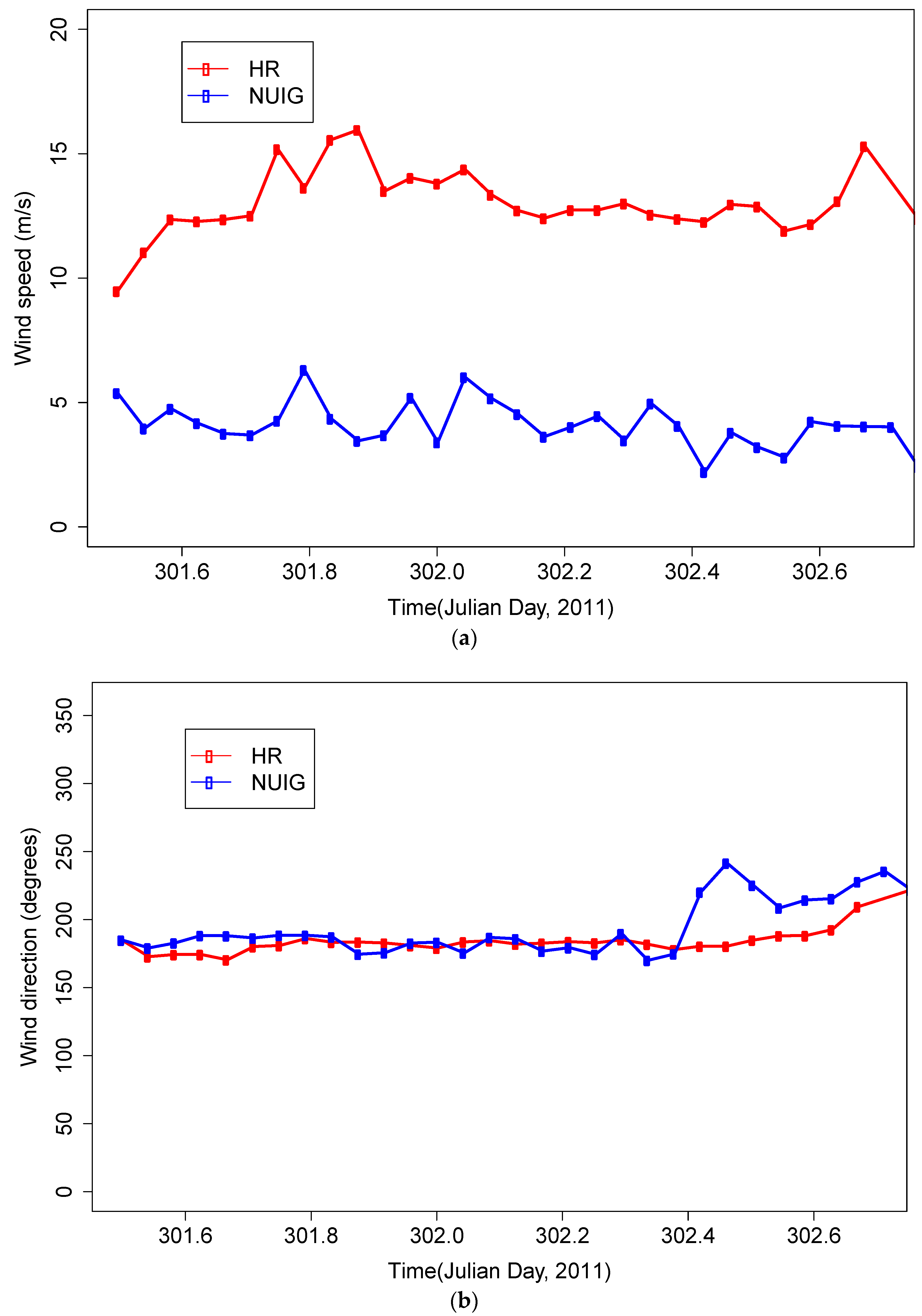
A comparison of wind speed and wind direction between the forecast high-resolution wind field and NUIG data during a sample 28-h period is shown in Figure 2. While the wind directions as shown in Figure 2b are similar, the offshore HR wind speeds as shown in Figure 2a were consistently higher than the land-based NUIG measurements. The largest variation of wind direction between HR and NUIG data occurred around Julian Day 323.4–302.55. This is most likely due to spatial variability in the wind field; the onshore NUIG wind station is approximately 13 km northeast of C1. The maximum wind speed recorded by IRUSE for the analysis period was around 7 m/s while the maximum offshore-modeled wind speed was around 14 m/s. In the following sections, the measured onshore wind data are referred to as the NUIG data; offshore data are referred to as HR wind fields. To better understand the similarities/variances between the NUIG and HR wind datasets, statistical analyses of the data were conducted for the 194 h where HR data were available. The analyses were conducted for four different offshore locations (marked C1–C4 in Figure 1) and the averages taken. These are presented in Table 2 along with the corresponding standard deviations. The mean difference in wind speed was approximately 7.4 m/s with a standard deviation of 1.4 m/s. This indicates that significant variation exists between the onshore and offshore wind speeds. By comparison the mean difference in wind direction was only 0.9° with a standard deviation of 18.7° indicating very little difference in offshore and onshore wind directions.
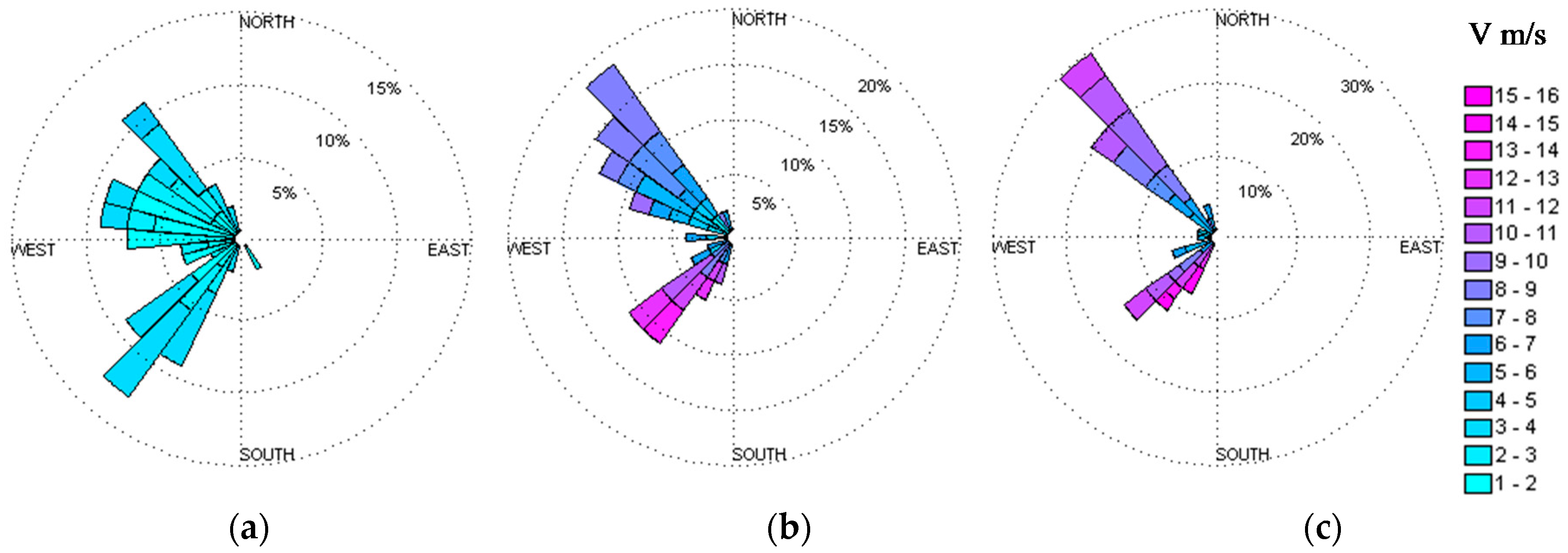
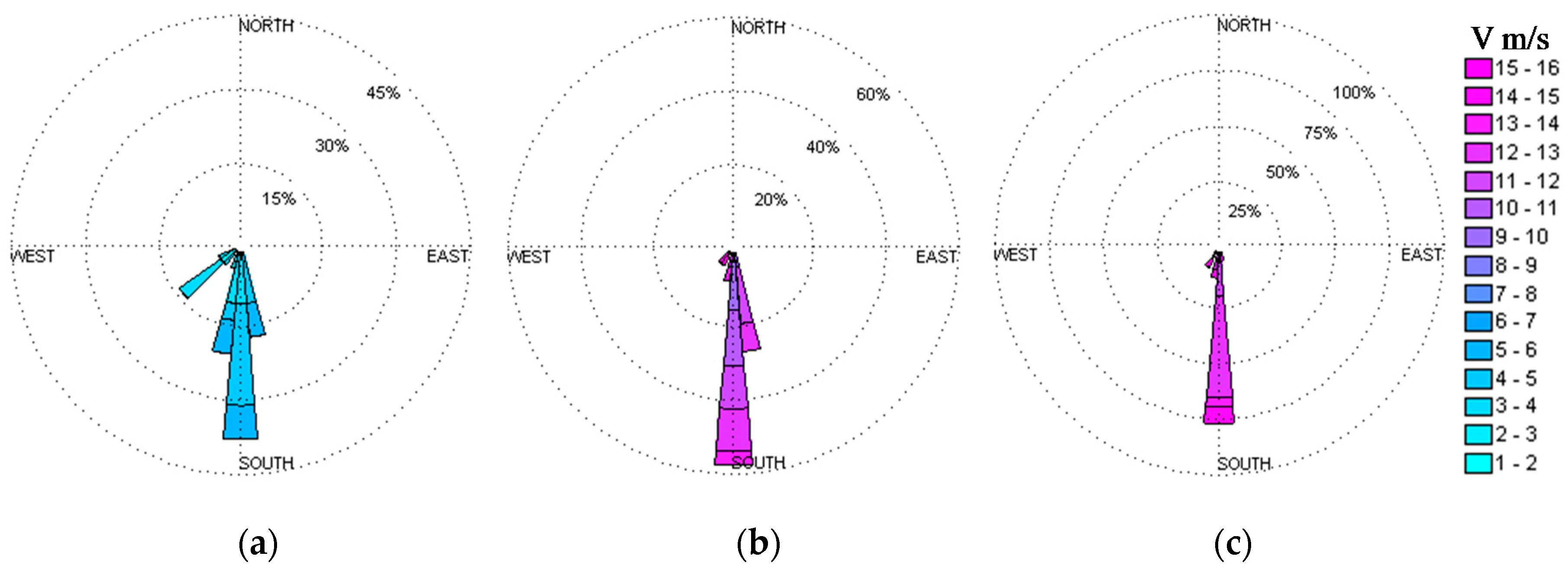
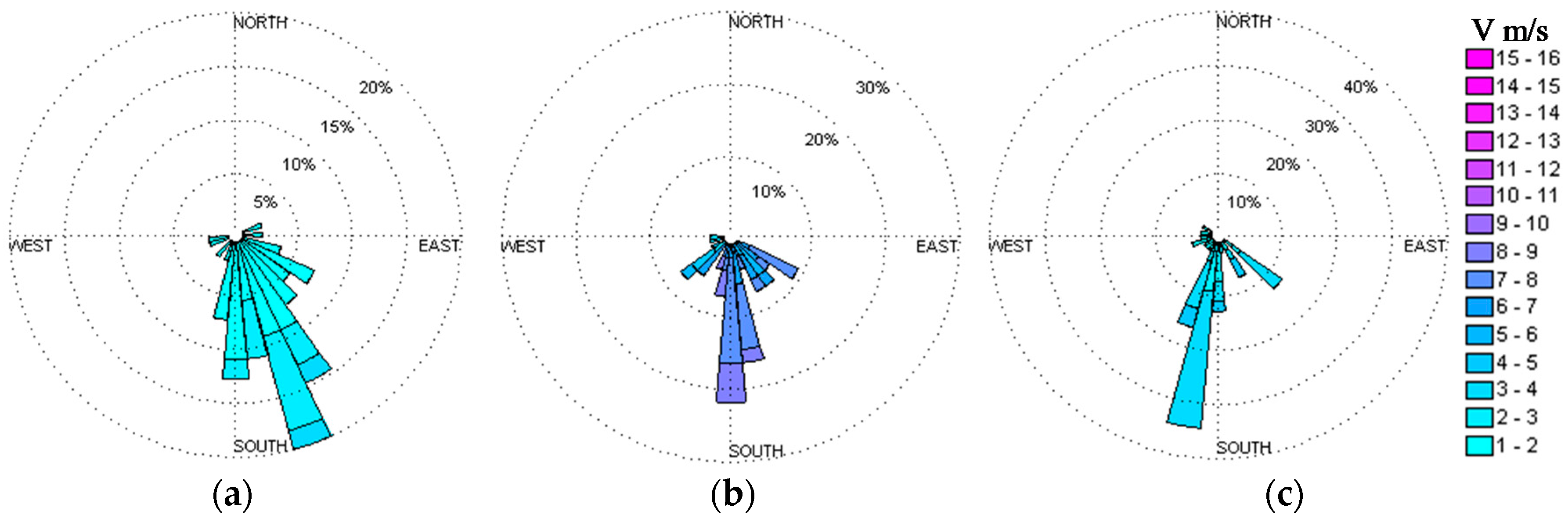
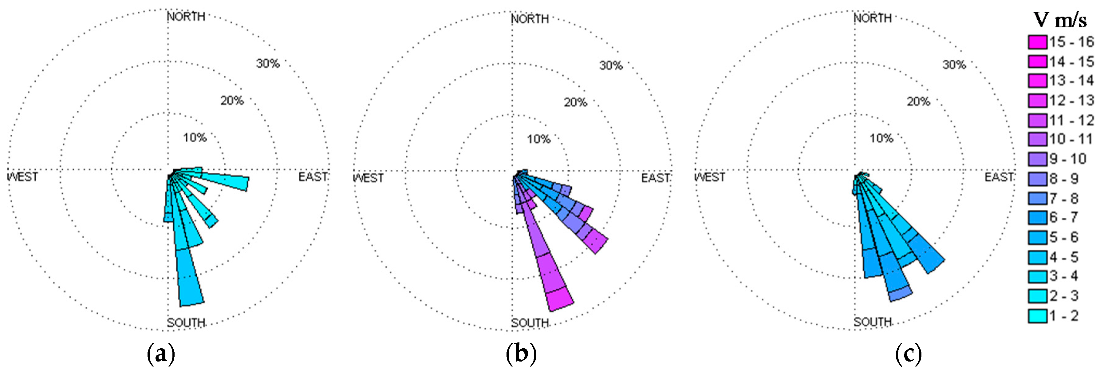
Figure 3, Figure 4, Figure 5 and Figure 6 compares wind roses between the onshore measured NUIG winds and offshore-modeled HR winds at two offshore locations, C1 and A2, for the above four time periods. The wind directions depicted in the wind roses were the directions from which the winds were blowing. There was relatively good agreement between the onshore measurements and offshore forecasts for wind direction; however, there were substantial differences in wind speeds. Wind direction was shown to be fairly consistent across all four periods with the NUIG measured wind showing the largest directional variation between the samples. This was most likely due to obstructions encountered on land.
Wind roses of panels (b) in Figure 3, Figure 4, Figure 5 and Figure 6 show that location C1 had higher wind speeds throughout the four periods. On the other hand, the wind direction at location A2 shows the least variation in wind direction. Due to their ready availability, and the lack of offshore data, land-based wind measurements are often used to provide surface boundary conditions in hydrodynamic models; however, this comparative study shows that offshore winds can be significantly different from onshore measurements. As a result, both datasets were used to separately force the numerical model of Galway Bay in order to determine improvements in accuracy as a result of using offshore rather than onshore wind conditions.
4. Measurements of Water Currents
4.1. ADCP Data
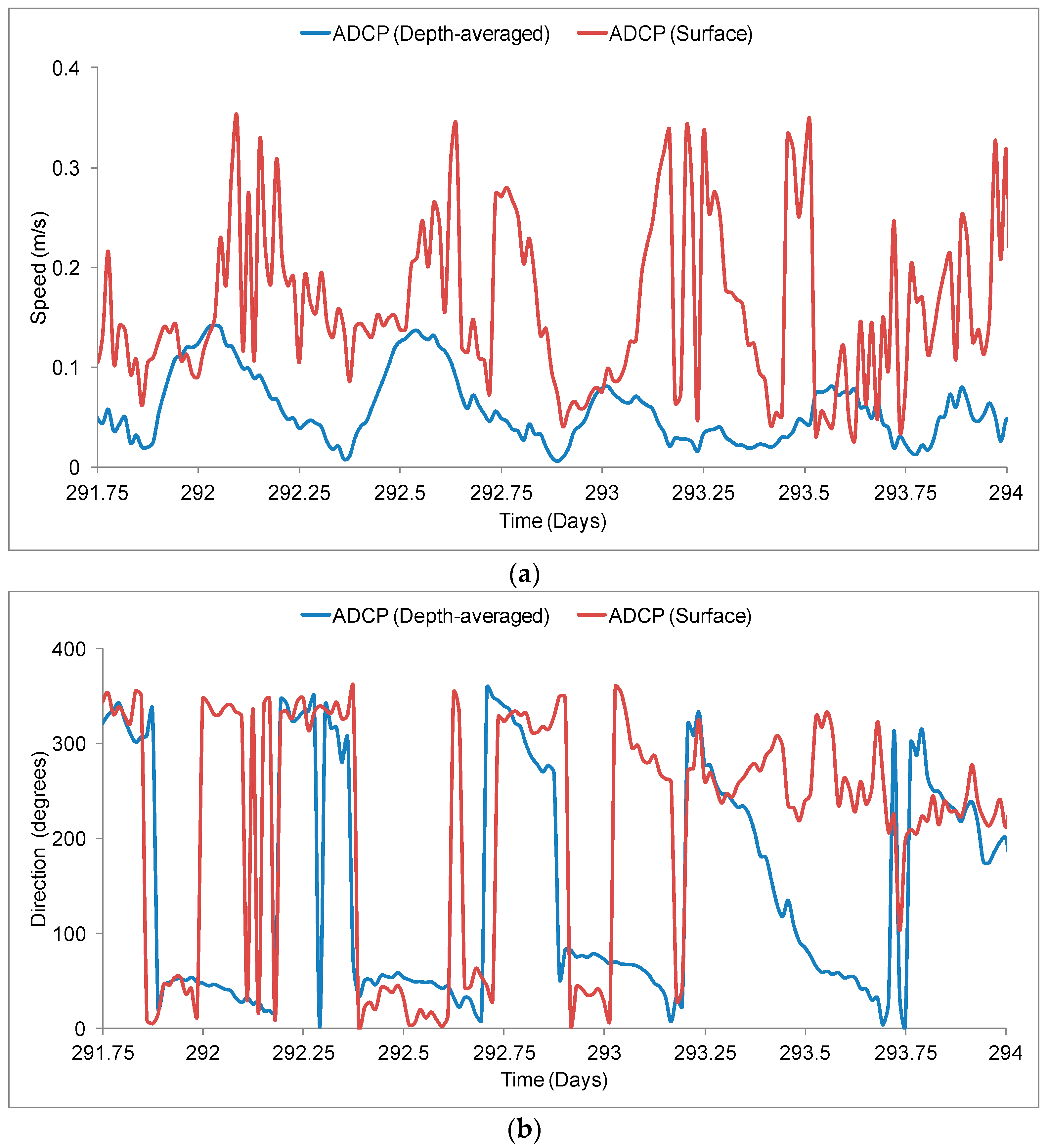
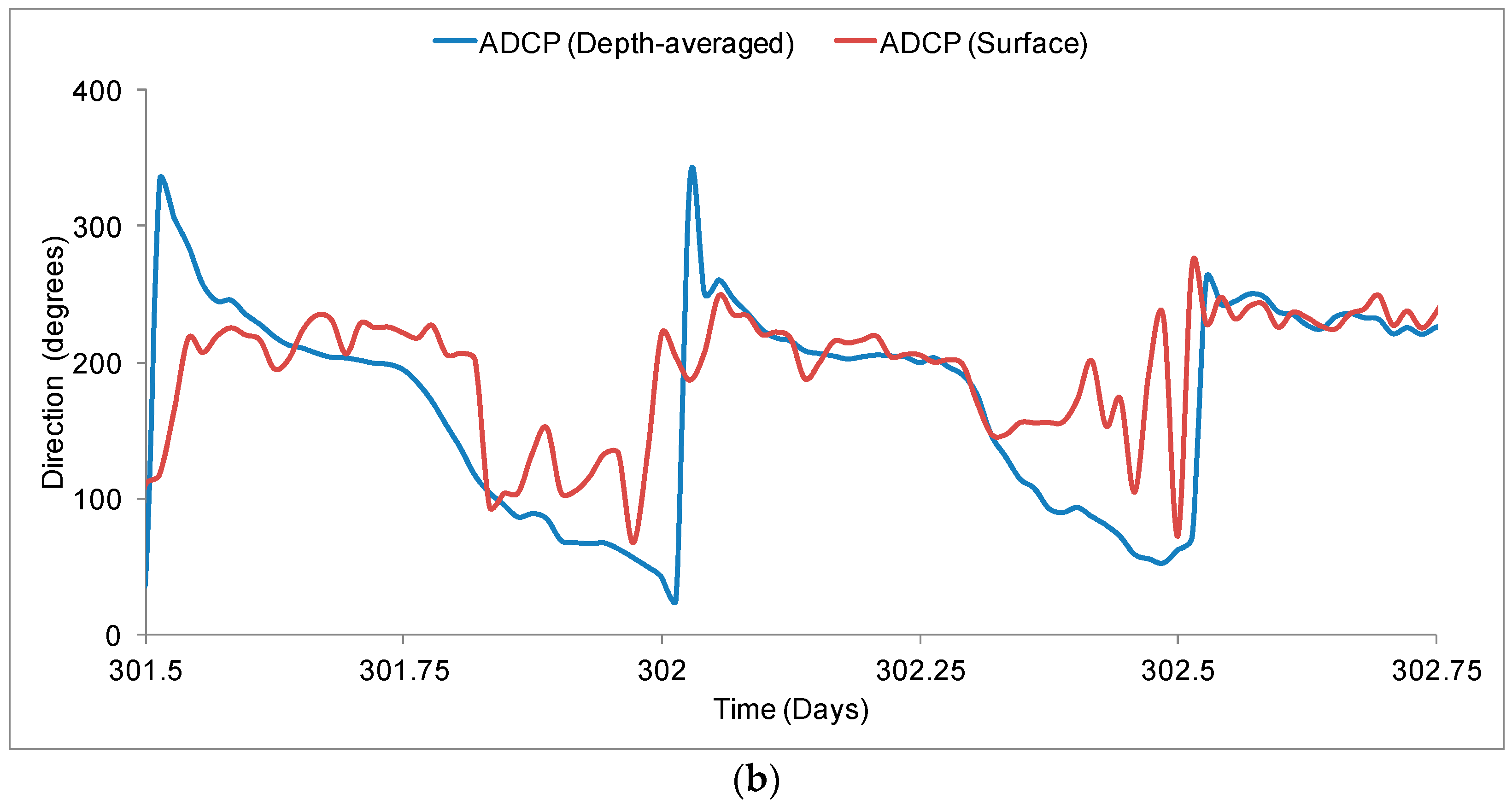
Data from a pair of Acoustic Doppler Current Profiler (ADCP) deployed in Galway Bay were analyzed for evidence of wind effects. ADCP velocity profiles are often used to characterize tidal currents [18]. The locations of the ADCPs are shown as A1 and A2 in Figure 1. The instruments were anchored to the sea floor and measured current speeds and directions through layers (bins) of equal depth throughout the full depth of the water column. The operating frequency of the RDI Teledyne Workhorse Sentinel ADCPs deployed in Galway Bay is 600 kHz. ADCP accuracy diminishes with distance from the instrument and readings are usually least accurate in the surface bin. Thus, in this research the ADCP surface velocities used were those just below the surface bin. To investigate the presence of wind-driven surface currents, the ADCP surface currents were compared with the depth-averaged ADCP velocities. Depth-averaged velocities were computed by averaging the velocity readings across 29 of the 30 2 m thick measurement bins that extended from 4–34 m from the seabed. Due to the accuracy issues mentioned previously, the surface bin was excluded from the depth averaging. The ADCP data were analyzed for two time periods, P1 and P2, when both measured and modeled wind data were available. The time series in Figure 7 and Figure 8 compare speeds and directions of the depth-averaged velocities computed from the ADCP data with the near-surface current velocities at ADCP location A2 during P1 and P2, respectively. The offshore wind speed and direction at location A2 during the ADCP velocity comparison time periods are shown in Figure 9 and Figure 10, respectively. Onshore NUIG wind data are also included for reference.
Figure 7a shows that the maximum current speeds at the surface layer of the water column can be as much as 50% greater than depth-averaged speeds. Similarly large differences in current speed are observed in Figure 8a. The directional plot shown in Figure 7b displays the variance between the surface current direction and depth-averaged current direction. The depth-averaged trajectory shifts generally in concert with flood-ebb tidal changes in Figure 7a; however, the same tidal signal is not as clearly visible in the direction of the surface currents. It is assumed that this is due to effects of the wind forcing observed in the current speeds. The winds during the period P1 were predominantly from the southwest while for P2 the winds are from the south. The direction of the surface currents (Figure 8b) does not act as one would expect, keeping a very steady direction with only a slight change corresponding to depth-averaged direction. This steady direction is most likely due to the constant wind direction (southerly) as shown in Figure 10.
The ADCP data clearly show that multi-layered circulation occurs in the Outer Bay (A2) with wind being the predominant driver of the surface layer and the tidal influence being the main driver of the lower water column layers. This type of compound circulation is not uncommon along the European Continental Shelf [19].
4.2. CODAR System
The high frequency CODAR radar system installed in Galway Bay provides near real-time measurements of surface currents at 300 m spatial resolution and one-hour temporal resolution. It is the only one of its kind in Irish or UK waters. The two radar masts are located at Spiddal and Mutton Island, and combine to give current vector maps that cover most of the Inner Bay (see points R1 and R2 in Figure 1). The two radars, which operate at a frequency of 25 MHz, measure continuous radial vector components at an effective depth of 0.48 m [20]. Bandwidth of both radars is 500 kHz. The data are transmitted directly to a central data management platform located at National University of Ireland, Galway [21].
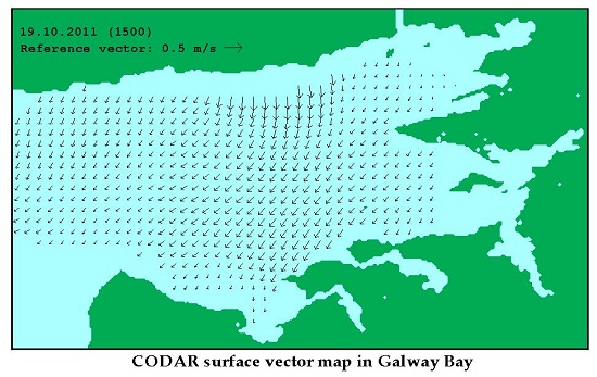
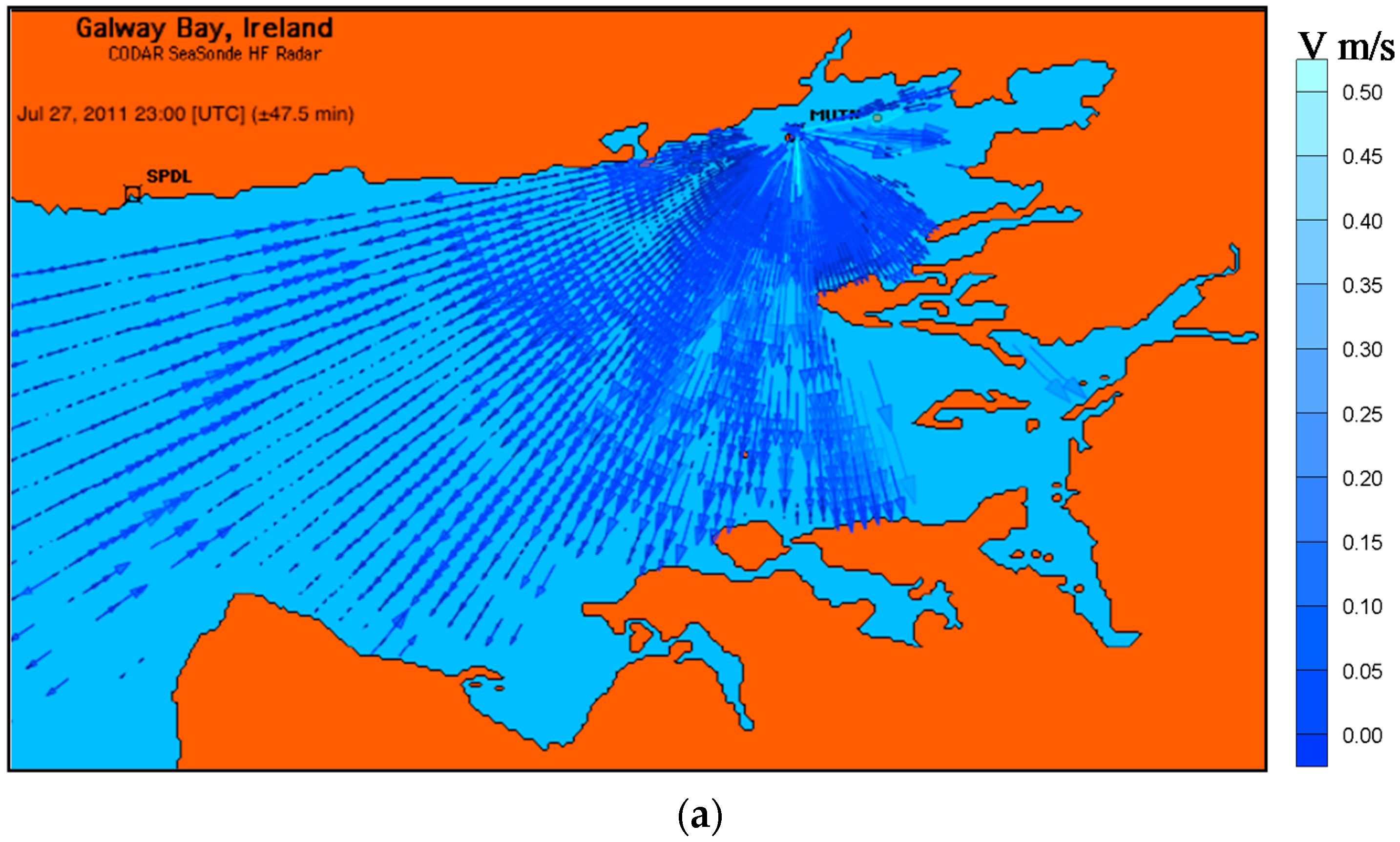
The CODAR system uses the theories of Braggs scattering and Doppler Shift to determine the surface currents from the backscattered radio wave. The Doppler shift explains the change in frequency of a signal scattered off a moving object. Doppler theory can be used to determine if a scattering object is moving toward or away from an observer as well as the speed at which it is moving [22,23]. By measuring the return signal, the CODAR system can determine the speed of the ocean waves that scattered the signal [24,25,26]. From this, wave speed can also be calculated [27,28,29,30]. Total surface current vector maps can be produced from at least two radar stations collecting radial components of the surface water velocity [31]. In this work, total surface currents were used to study effects of wind field resolution on coastal surface flow fields. Figure 11 shows a sample radial vector map from Mutton Island radar station and combined total surface vector map for Galway Bay.
5. Numerical Model
The Environmental Fluid Dynamics Code (EFDC) is a finite difference model, developed by Hamrick [32], which can simulate three-dimensional flows and transport processes in surface water systems, rivers, lakes, estuaries, wetlands and coastal areas. The model structure includes four major modules: (1) a hydrodynamic module, (2) a water quality module, (3) a sediment transport module, and (4) a toxics module. In this study, only the hydrodynamic module was used. The EFDC model solves the three dimensional, vertically hydrostatic, free surface, turbulent-averaged equations of motion for a variable density fluid. The model uses a stretched (sigma) vertical coordinate system and a Cartesian, or curvilinear, orthogonal horizontal coordinate system [33,34,35]. The EFDC model has been widely used to simulate hydrodynamic processes in marine waters [36,37].
Vertical boundary conditions for the momentum equations are kinematic shear stresses at the water bottom (z = 0) and water surface (z = 1). Expressions for the bottom and surface shear stresses, respectively, are [38]:
where , are shear stresses at the bottom (z = 0) and shear stresses at the surface (z = 1), respectively (N/); H is water depth (m); , are wind speed components at 10 m above the water surface (m/s); kb is bottom drag coefficient; is wind-stress coefficient; refers to east-west and north-south velocity components computed at mid-height of the bottom layer respectively (m/s). The bottom drag coefficient is computed using:
where κ = 0.4 is the von Karman constant; is the dimensionless thickness of the bottom layer; is the dimensionless bottom roughness height; is the bottom roughness height (m). Specification of the kinematic shear stresses highly depends on the correct approximation of the wind-stress coefficient. The default wind-stress coefficient is calculated according to Wu [39] as:
The wind-stress formulation used in the EFDC model to date has been derived from observations of a large number of data sets from different studies which all used wind-stress coefficients estimated from data collected in the open oceans [39]. The effects of surrounding topography and/or irregular bathymetry might cause significant errors, for example, if an estuary was sheltered. It was suggested that the wind-stress formulation used in the EFDC model held best for winds in the range of 8–20 m/s. Errors may occur when using this wind-stress coefficient for very high or low wind conditions [39]. However, Wen [13] found that a constant wind-stress coefficient kw = 2.6 × 10⁻³ produced good results for a previous Galway Bay modeling study. This constant value of wind-stress coefficient was therefore also used in the present study.
A variable vertical layer structure, where layers are thinnest at the surface and seabed and increase toward the middle of the water column, was applied in the EFDC model for Galway Bay. This configuration has been found to ensure that the wind effects can be transferred from surface to deeper layers in 3D models [40]. To assess the effects of data used for wind forcing, both NUIG onshore wind data and modeled offshore HR wind data were separately used to force the model. Other meteorological forcing data such as temperature, rain, solar radiation and relative humidity were obtained from the weather station IRUSE located at campus of National University of Ireland, Galway at one-minute interval. Records of river flows for the River Corrib, which enters Galway Bay north of point R1 in Figure 1, were obtained from the Office of Public Works. Water elevation time series generated from Oregon State University Tidal Prediction Software (OTPS) were used to define the tidal forcing on the western and southern open boundaries in the model [41,42]. The water elevation along open sea boundaries was constant in space and variable in time.
In order to validate the hydrodynamic model, the 30-day period from 14 October–14 November 2011, was chosen when a full set of wind and CODAR data were available for the Bay. In order to evaluate the improvements of model results by considering more accurate wind forcing, three separate model scenarios as shown in Table 3 were implemented.
6. Results
6.1. Velocity Components
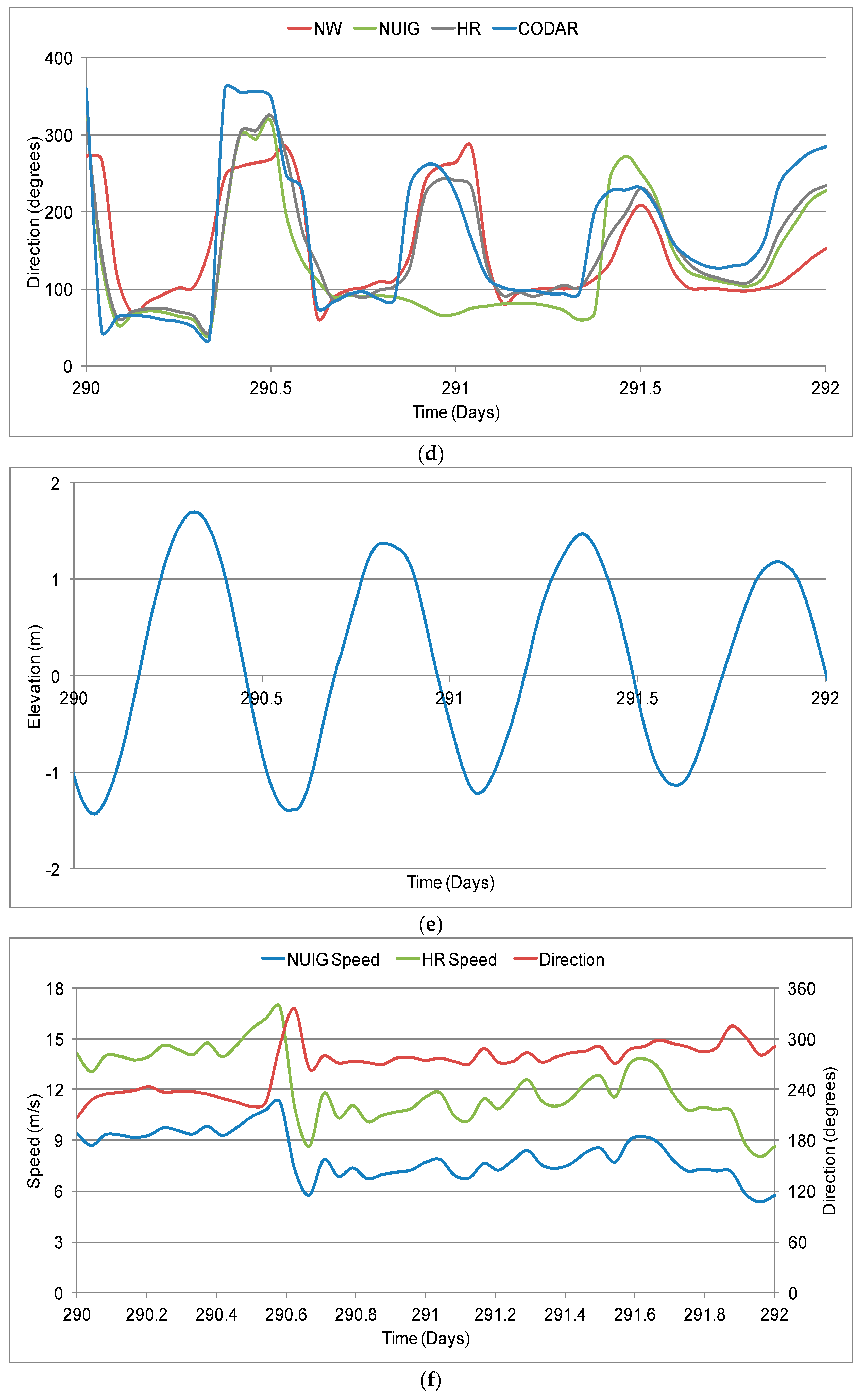
The representative model results (time series of surface velocity components, total surface speed and direction) with different types of wind fields are shown in Figure 12 and Figure 13 at location C3 for different time periods, respectively. Figure 12 compares modeled and measured surface currents at C3 over Period 1.
The wind-forced models performed well in simulating observed field conditions at C3. Predicted velocity magnitudes and directions were generally in good agreement with observed data (Figure 12c,d, with the model HR fitting better with CODAR observed profiles than the model NUIG. The east-west (u) and north-south (v) surface velocity components for the model HR simulations shown in Figure 12a,b respectively, pick up the general trend followed by the CODAR observed vector components. The directional shift previously noted at location C3 can be seen clearly at time 290.5 days in Figure 12d,f. The model HR ability to follow the trend of north-south surface velocity component of CODAR data is very favorable. Statistics of RMSE between model results and radar data at location C3 during P1 are presented in Table 4. Figure 13 compares modeled and measured surface currents at C2 during P3.
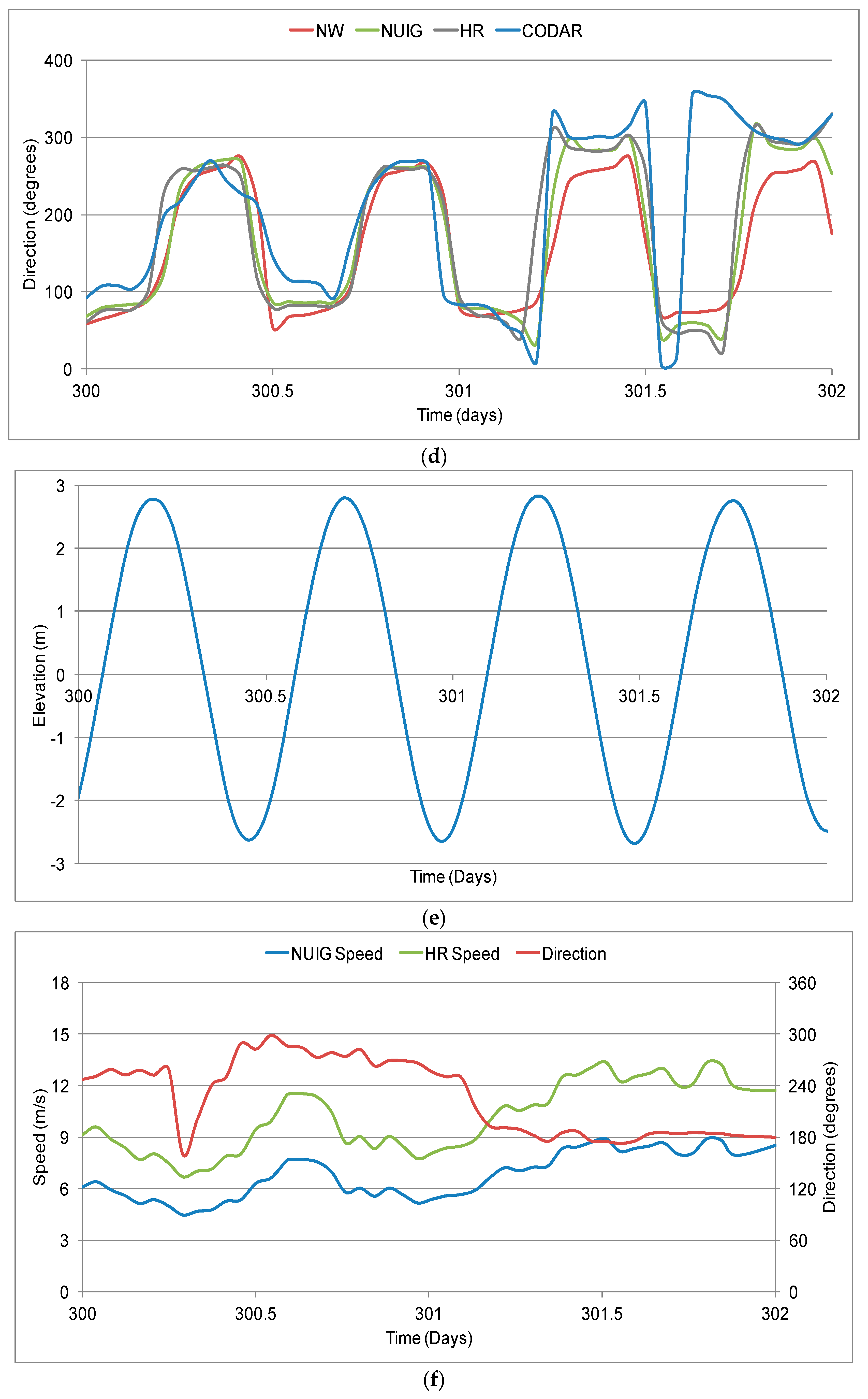
The east-west surface velocity component for both modelled and observed values above is generally in good agreement, with a strong tidal signal visible. The east-west surface velocity component of CODAR data observed for the flooding tide around 301.6 days differs significantly from the recorded values for the preceding flood tides. The measured tide appears to have no easterly component (positive u values correspond to easterly components). The current direction plot proves this as the CODAR direction for the flood tide in question is approximately 360°, i.e., north. The prevailing winds for this period were from the south which would indeed impart a northerly component to the surface currents. The prevailing speeds were also quite high (12–13 m/s), which completely dampened the tidal influence on the surface waters and generated strong northerly flows. As for the east-west surface velocity component plot, the wind-driven models do show some reduction in peak flood velocities at this time and the magnitude of the reduction is greater for the higher wind speeds of the model HR.
In order to statically assess the modeled results for the different wind boundary conditions, Room-Mean-Squared-Error (RMSE) between radar surface currents and modeled results and square of the Pearson product moment correlation coefficient (RSQ) for both surface velocity components were computed for each velocity component at two locations C2 and C3, as shown in Table 4.
The tabulated RMSEs in Table 4 confirmed that the wind-forced simulations were greatly improved in relation to CODAR observed currents relative to no wind forcing and that in the model HR was more accurate than the model NUIG. At C3, during P1, RMSEs of the model HR in north-south and east-west surface velocity components were 34% and 14% lower, respectively, than those for the model NUIG. At C2, during P3, RMSEs of the model HR in north-south and east-west surface velocity component were also 8% and 4% lower than those of the model NUIG. This suggests that using spatially varying wind fields specifically forecast for the offshore region enabled the model to better capture surface flow patterns than using a non-spatially varying wind field based on onshore coastal measurements, as would be quite common in coastal modeling studies. Moreover, although the model application of onshore winds (model NUIG) improved modeling performance of surface velocity components in comparison with model NW. This indicated that it was favorable to apply wind data to simulate surface flow fields, especially using spatially and temporally varying wind data. Additionally, RSQ values for both surface velocity components increased at C3 during P1 when finer wind data were applied. This further indicated that consideration of wind forcing enhanced modeling performance in comparison again the model without wind, and utilization of spatially and temporally varying wind data generated better correlation with observations than models using spatially constant wind data and no wind data. Similar increasing trend of RSQ values occurred for east-west surface velocity component at C2 during P3, but it was as significant as at C3 during P1. However, improvement extent of RSQ in north-south surface velocity component was significant when wind force was considered.
To summarize, the qualitative and quantitative analyses presented above show that the level of agreement between modeled surface currents and those recorded by CODAR were significantly better when wind was included in the model and that the model HR, with spatially varying offshore winds applied, gave better agreement with CODAR data than the model NUIG which used land-measured winds, especially during strong wind events.
6.2. Vector Fields of Surface Currents
The previous section compared time series between modeled results and CODAR data to determine the performance of the different model simulations at discrete locations in Galway Bay. In order to examine how the model HR simulates vector fields in space. Depth-averaged and surface current vector fields from model NW were compared with CODAR observation, surface vector fields from model HR to assess the effects of wind on surface currents and the relative accuracies of the wind-driven models.
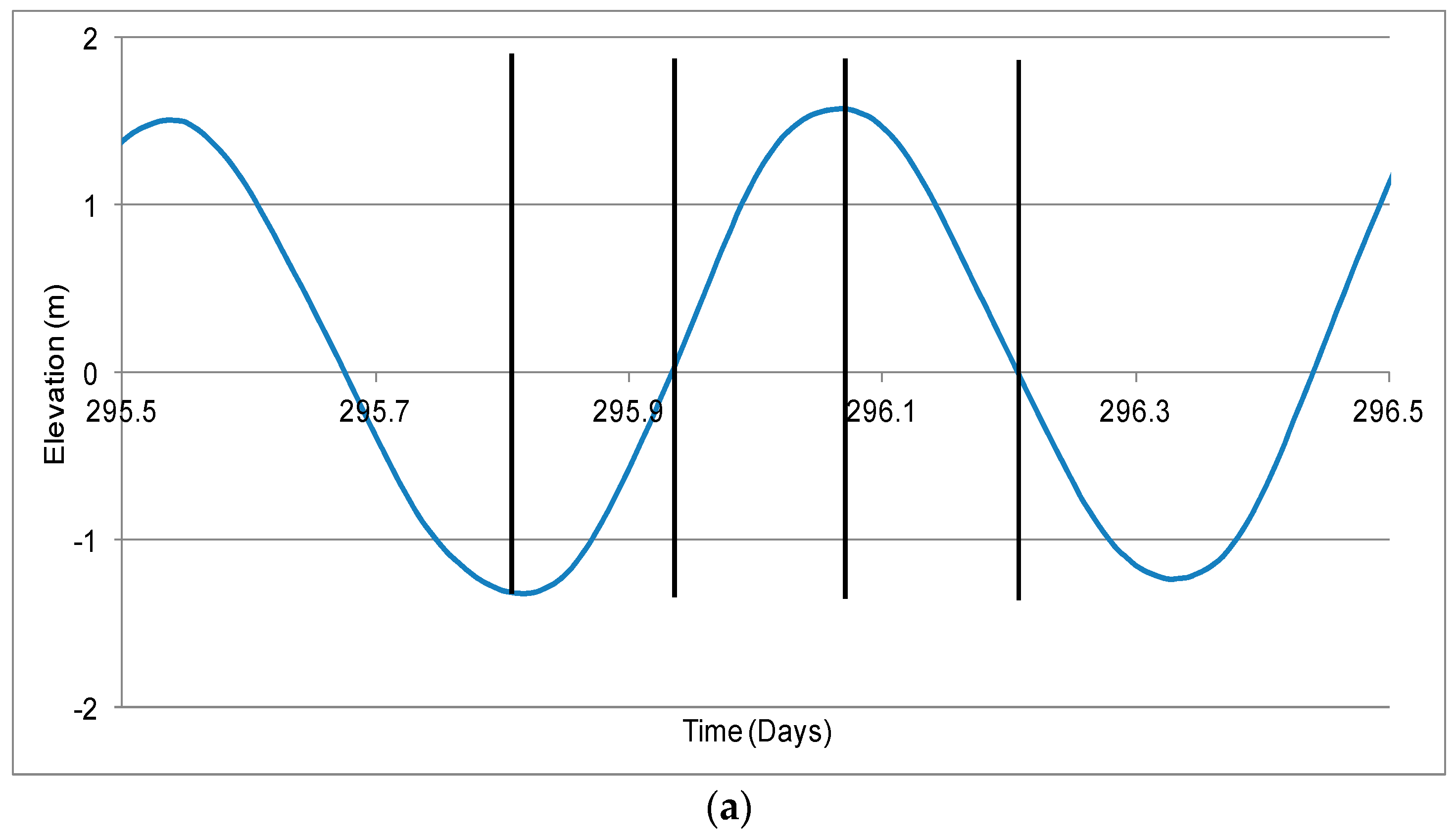
The comparison was conducted on neap tides when the effect of wind forcing relative to tidal forcing was found to be greater and at a time when winds were blowing from the south, i.e., perpendicular to the prevailing east-west tidal movements. Vector fields were generated from the data at four different stages of the tide over the course of a neap tidal cycle: low water (LW), mid-flood (MF), high water (HW) and mid-ebb (ME). Figure 14 shows the time steps of comparison and the corresponding prevailing winds. The prevailing wind speed during the period of comparison was approximately 9 m/s from the south.
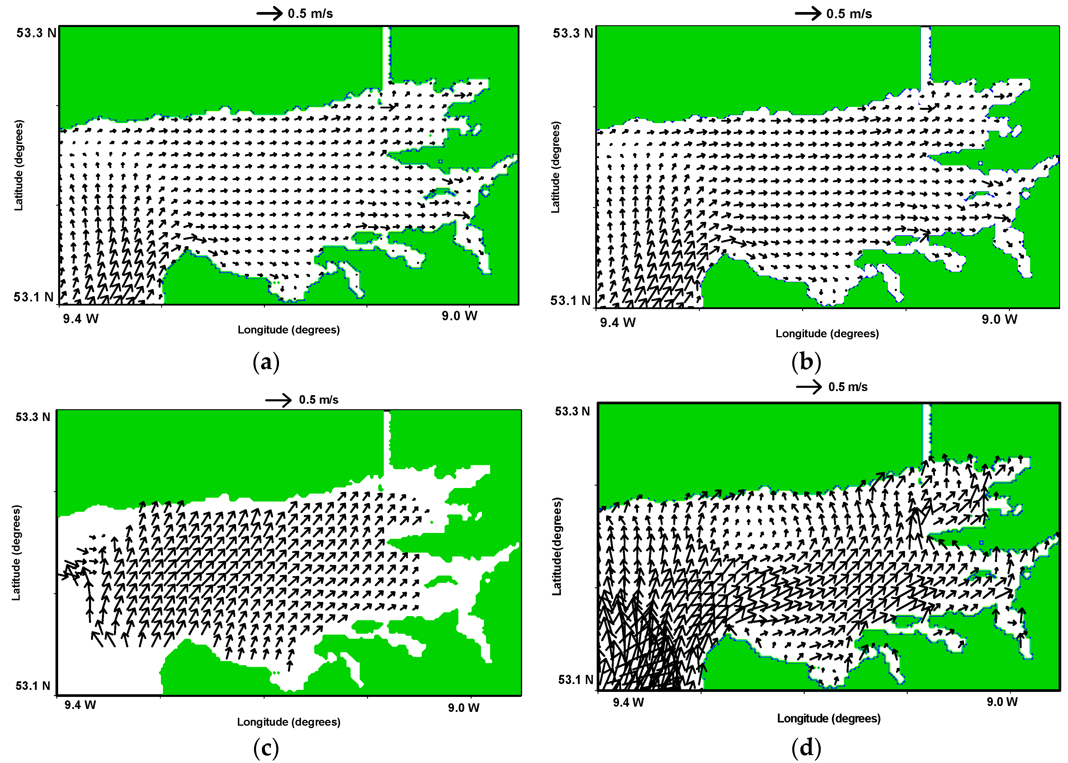
Figure 15, Figure 16, Figure 17 and Figure 18 compare the measured and modeled current vector fields at the times of low water, mid-flood, high water and mid-ebb, respectively. The first point of note was the similarity between the surface and depth-averaged current vectors fields in model NW; this was expected given the absence of any wind forcing. The only difference, again as it should be, was that the surface currents were slightly greater in magnitude. The second general point of note was the clear difference between all of the CODAR and model HR flow fields in comparison to the corresponding surface flow fields from model NW. These differences clearly demonstrated the significant role of wind in the generation of surface currents in the bay.
At low water (Figure 15) the depth-averaged vector fields from model NW shows very little circulation occurring within the Inner Bay. This is as would be expected since the times of low and high water in a coastal embayment typically corresponds to the times of slack water. In the absence of wind, the surface vector field of model NW also shows very little hydrodynamic activity with surface currents close to zero in much of the Inner Bay. The CODAR vector field shows that the stresses generated by the prevailing winds are sufficient to generate movement of the surface layer. For the eastern and central parts of the Inner Bay the direction of flow is to the north, due to the prevailing southerly winds. In the northeast of the Bay, CODAR shows southerly flows and in the southeast it shows westerly flows. These flows may be due to local wind effects, or in the case of the southerly flows in the northeast the freshwater influence of the Corrib River. The surface vector fields of model HR also shows northerly flows in the north half of the bay; however, it also shows easterly flows in the southeast, which do not agree with CODAR. It is interesting to note that the surface vector fields of model HR and CODAR appear to form an anti-clockwise gyre in the Outer Bay. The formation of this gyre was in agreement with studies carried out by [6].
At the time of mid-flood (Figure 16), the depth-averaged and surface vector fields of model NW show strong easterly flows in the Inner Bay and as they are very much dominated by the tidal forcing. The CODAR surface vector plot in Figure 16b shows strong northeasterly flows with the northern component of the flow contributed by the southerly winds. The HR surface vector plot shows considerable similarity to the CODAR plot across the majority of the Inner Bay with the exception of the southern coast where the HR flows are more easterly and the CODAR flows are more northerly. Given the levels of agreement elsewhere, this disagreement is most likely due to differences between the actual wind field in that area and the predicted wind field used in the model HR. Surface vector fields of COADR and model HR show splitting of the southerly flow from the Outer Bay as it enters the Inner Bay some of the flow entering the Inner Bay and the remainder circulating, in an anti-clockwise direction, back out to the Outer Bay.
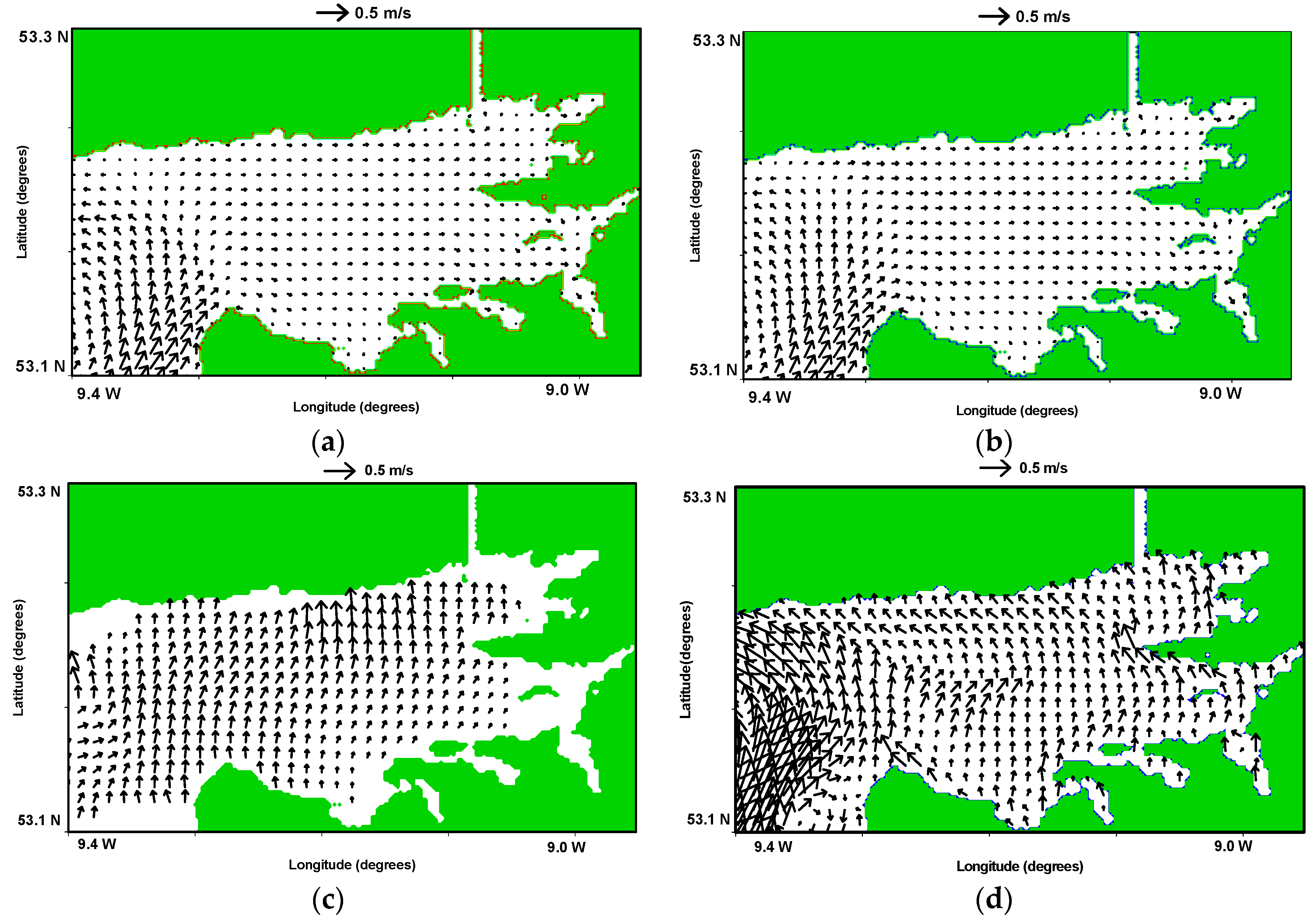
At the high tide time step in Figure 17, the depth-averaged and surface vector fields of model NW are seen to be quite similar to the surface vector fields at low water level with very little hydrodynamic activity in the Inner Bay. Once again as shown in Figure 17a at a time of model NW shows very little circulation occurring within the Inner Bay. As for surface flow fields at low water level, the anti-clockwise gyre is clearly visible in the Outer Bay. The CODAR surface vector field shows northerly flows that were driven by the southerly winds. The model HR reproduced quite accurately as CODAR data. In the Outer Bay the HR current vectors are of greater magnitude than the CODAR vectors but it should be noted that the accuracy of the CODAR observations was known to be lower in this area due to the small angle of intersection of the radials from the two observation stations. The anti-clockwise circulation pattern in the Outer Bay is visible in both the surface vector fields of model HR and CODAR.
At mid-ebb (Figure 18), both the NW depth-averaged and surface currents show a very strong westerly component under the primary influence of tidal forcing. By contrast, both the CODAR and HR vector fields show strong northwesterly flows throughout the Inner Bay. The HR vectors are again in very close agreement with the CODAR vectors, even down to reproducing the westerly flows in the northeast of the bay, which is most likely due to the influence of the Corrib River. Difference of vector fields between CODAR data and model HR occurred near southwest corner as shown in Figure 18c,d. Given the levels of agreement elsewhere, this disagreement is most likely due to differences between the actual wind fields in that area and the predicted wind field used in the model HR.
In summary, the general directions and trends displayed by both the CODAR and modeled vector fields for four different stages of the time have been considered. Surface vector fields indicate that the surface currents within the Inner Bay at the time of inspection were largely dominated by wind and that the numerical model was capable of simulating some of this wind influence. Model HR produced closer patterns of surface vector fields to CODAR measurements than model NW and model NUIG.
7. Discussion
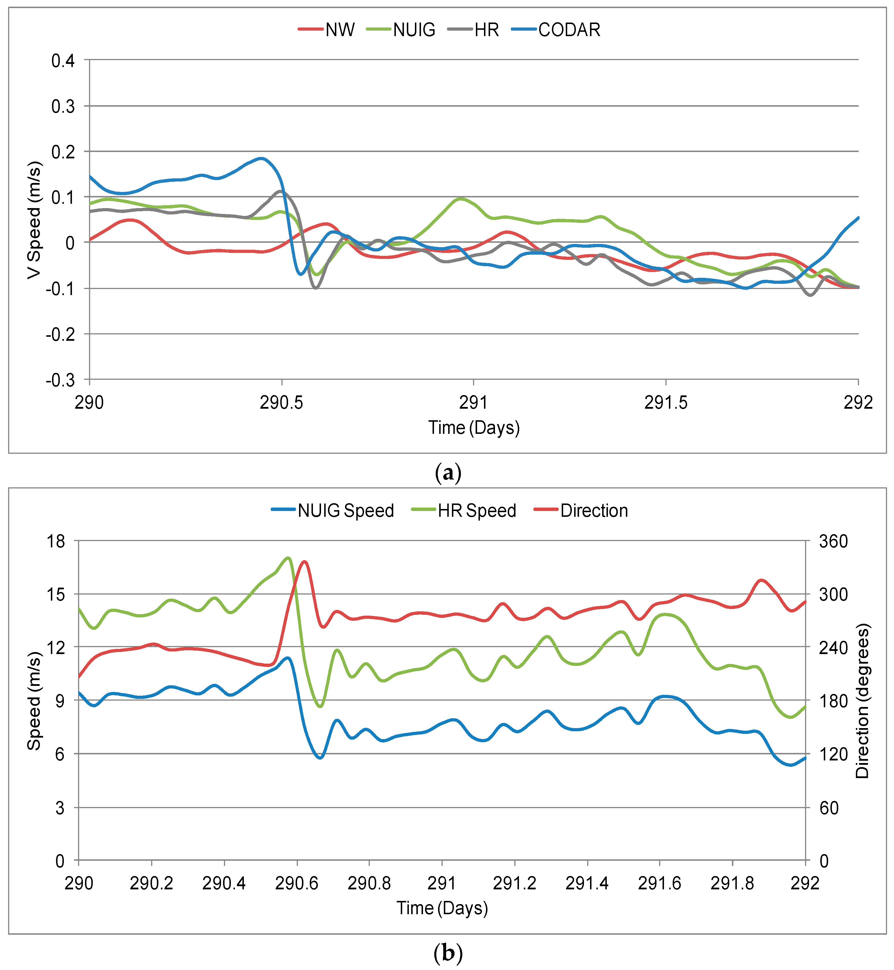
Since the tidal forcing entering and leaving Galway Bay is mainly east-west in direction, the predominant directions of tidal currents are east-west [14]. This was evidenced by the modeled east-west surface velocity components that contained a very strong tidal signal and did not experience significant changes under different wind conditions. The effect of wind direction on the surface currents was most clearly evident on the north-south surface velocity component. In order to further explore this aspect of circulation, the comparison of measured and modeled north-south surface velocity components at C3 are shown in Figure 19.
The shift in wind direction shown in Figure 19b at approximately Day 290.5 is seen to have had a direct influence on both the measured CODAR V-component. When wind was included in the model (NUIG_V and HR_V), the wind produced similar effects on the north-south surface velocity components. However, when wind forcing was omitted from the model, the velocity was much more constant, as one would expect under conditions of tidal forcing only. This indicated that consideration of wind forcing enhanced the model performance, especially for north-south surface velocity component. Surface vector fields in Figure 19a show that the surface layer circulation within Galway Bay was strongly correlated with wind speed and direction. The ability of the model to reflect the measured surface currents movements confirms the influence of wind in Galway Bay.
Previous research on circulation in Galway Bay has shown through drifter studies [6] and current meter readings [43] that the effect of wind is dominant in the upper layer of the bay. Double layered circulation due to wind direction, has been recorded at both the South Sound and the Foul Sound from current meter readings taken by Fernandes [43]. The surface drifter study by Booth [6] showed a direct flow from the Outer Bay into the Inner Bay, which coincided with prevailing winds at time of deployment. Nolan [7] found that winds emanating from the north and east are more likely to assist the Corrib River plume along the north shore, while winds from the south and west (prevalent winds in the bay) impeded the progression out of the bay. It was recorded that under prolonged southwester winds, a build-up of fresh water occurred, which began to mix vertically rather than horizontally. The location of the gyre within the Outer Bay of Galway Bay has been recorded by both Booth [6] and Fernandes [43], and was reinforced by mineral deposits found in the Outer Bay [44] and ultra violet absorbance values taken by Fernandes [43].
8. Conclusions
The upper layer circulation of surface currents in Galway Bay has been shown to be primarily strongly influenced by wind. The EFDC model was used to simulate coastal circulation in in Galway Bay. Three model scenarios with different types of wind sources: (a) no wind (NW); (b) temporally varying but spatially non-varying measured onshore wind (NUIG); (c) temporally and spatially varying offshore wind forecast offshore wind (HR), were implemented. The modeled results were validated through comparison with measured ADCP and CODAR data. The main results from the research are:
- (1)
- Forecasted high-resolution (HR) wind data for the offshore generally had similar trend in direction as the measured NUIG onshore wind data; however, the offshore HR wind speeds were consistently higher than the land-based NUIG measurements. The mean difference in wind speed for the 30-day simulation period was approximately 7.4 m/s with a standard deviation of 1.4 m/s. This indicates that significant variation exists between onshore and offshore wind speeds, and so where possible, offshore winds should be used as boundary conditions for coastal hydrodynamic models.
- (2)
- Analysis of ADCP data showed that multi-layered circulation occurs in the area with wind being the predominant driver of the surface layer and the tidal influence being the main driver of the lower water column layers.
- (3)
- Comparison of surface velocity components time series showed that the level of agreement between modeled surface currents and those recorded by CODAR were significantly better when wind was included in the model and that the HR model, with spatially-varying offshore winds applied, gave better agreement with CODAR data than both the NUIG model which used land-measured winds which in turn gave better agreement with CODAR than the NW model without wind included, especially during strong wind events. This wind forcing in an important boundary condition to consider.
- (4)
- Surface vector fields for four different states of the tide indicated that the surface currents within the Inner Bay at the time of inspection were strongly dominated by wind and that the numerical model was capable of simulating some of this wind influence, depending on the type of wind forcing specified. The model driven by winds, especially spatially varying HR wind fields, clearly produced better agreement with the measured surface current vectors. This agreement was most improved in the north-south surface velocity component (v).
In short, spatially varying winds (model HR) applied across the model domain produced better simulation of coastal circulations with measured ADCP and CODAR data than using spatially uniform winds (model NUIG) and model without winds (model NW). Thus, it is necessary to use spatially varying winds to simulate surface vector fields for Galway Bay area. This study also plays a reference role on modeling of surface flows in other study regions.
Acknowledgments
We would like to thank Informatics Research Unit for Sustainable Engineering (IRUSE) for providing the weather data, Oregon State University for providing the OTIS software, and Ireland’s High-Performance Computing Centre (ICHEC) for providing computation service and Met Eireann for allowing use of the wind model data. This article is an extension of the work presented at ICEER2017 and published in Energy Procedia.
Author Contributions
Lei Ren, Diarmuid Nagle conceived and ran models; Lei Ren, Diarmuid Nagle, Stephen Nash and Michael Hartnett wrote this paper.
Conflicts of Interest
The authors declare no conflict of interest.
Abbreviations
| ADCP | Acoustic Doppler Current Profiler |
| ARIMA | Autoregressive Integrated Moving Average |
| CODAR | Coastal Ocean Dynamics Applications Radar |
| EFDC | Environmental Fluid Dynamics Code |
| ECMWF | European Centre for Medium-range Weather Forecasting |
| HR | High resolution |
| HF | High-Frequency |
| HW | High water |
| ICHEC | Ireland’s High-Performance Computing Centre |
| IRUSE | Informatics Research Unit for Sustainable Engineering |
| LW | Low water |
| MF | Mid-flood |
| ME | Mid-ebb |
| NUIG | National University of Ireland Galway |
| NW | No wind |
| OTPS | Oregon State University Tidal Prediction Software |
| RMSE | Room-Mean-Squared-Error |
References
- Lewis, M.; Neill, S.P.; Robins, P.E.; Hashemi, M.R. Resource assessment for future generations of tidal-stream energy arrays. Energy 2015, 83, 403–415. [Google Scholar] [CrossRef] [Green Version]
- Brown, A.J.G.; Neill, S.P.; Lewis, M.J. The influence of wind gustiness on estimating the wave power resource. Int. J. Mar. Energy 2013, 3–4, 1–10. [Google Scholar] [CrossRef]
- Liu, X.; Lai, X.; Zou, J. A New MCP Method of Wind Speed Temporal Interpolation and Extrapolation Considering Wind Speed Mixed Uncertainty. Energies 2017, 10, 1231. [Google Scholar] [CrossRef]
- Yang, H.; Jiang, Z.; Lu, H. A Hybrid Wind Speed Forecasting System Based on a ‘Decomposition and Ensemble’ Strategy and Fuzzy Time Series. Energies 2017, 10, 1422. [Google Scholar] [CrossRef]
- Kim, J.-Y.; Kim, H.-G.; Kang, Y.-H. Offshore Wind Speed Forecasting: The Correlation between Satellite-Observed Monthly Sea Surface Temperature and Wind Speed over the Seas around the Korean Peninsula. Energies 2017, 10, 994. [Google Scholar]
- Booth, D. The Water Structure and Circulation of Killary Harbour and of Galway Bay. Ph.D. Thesis, National University of Ireland, Galway, Ireland, 1975. [Google Scholar]
- Nolan, G.D. A Study of the River Corib Plume and its Associated Dynamics in Galway Bay during the Winter Months. Master’s Thesis, University College Galway, Galway, Ireland, 1997. [Google Scholar]
- Nolan, G. Observations of the Seasonality in Hydrography and Current Structure on the Western Irish Shelf. Ph.D. Thesis, National University of Ireland, Galway, Ireland, 2004. [Google Scholar]
- Saboia, J.L.M. Autoregressive Integrated Moving Average (ARIMA) Models for Birth Forecasting. J. Am. Stat. Assoc. 1977, 72, 264–270. [Google Scholar] [CrossRef]
- Ho, S.L.; XIe, M.; Goh, T.N. A comparative study of neural network and Box-Jenkins ARIMA modeling in time series prediction. Comput. Ind. Eng. 2002, 42, 371–375. [Google Scholar] [CrossRef]
- Ren, L.; Sheahan, J.; Nash, S.; Nagle, D.; Hartnett, M. Estimation of the High Resolution Wind Field at Galway Bay. In Proceedings of the 2nd International Conference on Energy and Environment Research, Lisbon, Portugal, 13–14 July 2015; pp. 1–4. [Google Scholar]
- Nash, S.; Hartnett, M. Nested circulation modelling of inter-tidal zones: Details of a nesting approach incorporating moving boundaries. Ocean Dyn. 2010, 60, 1479–1495. [Google Scholar] [CrossRef]
- Wen, L. Three-Dimensional Hydrodynamic Modelling in Galway Bay. Ph.D. Thesis, University College Galway, Galway, Ireland, 1995. [Google Scholar]
- Ren, L.; Nash, S.; Hartnett, M. Forecasting of Surface Currents via Correcting Wind Stress with Assimilation of High-Frequency Radar Data in a Three-Dimensional Model. Adv. Meteorol. 2016, 2016, 1–12. [Google Scholar] [CrossRef]
- Dabrowski, T. A Flushing Study Analysis of Selected Irish Waterbodies. Ph.D. Thesis, National University of Ireland Galway, Galway, Ireland, 2005. [Google Scholar]
- Ding, J. Impact of HARMONIE High-Resolution Meteorological Forecasts on the Air Quality Simulations of LOTOS-EUROS; Royal Netherlands Meteorological Institute: De Bilt, The Netherlands, 2013. [Google Scholar]
- Perttula, T.; Jokinen, P.; Eerola, K. Impact of IASI in HARMONIE forecasting system during convective storm events in Finland during summer 2010. In Proceedings of the International TOVS Study Conference, Toulouse, France, 21–27 March 2012. [Google Scholar]
- Lewis, M.; Neill, S.P.; Robins, P.; Hashemi, M.R.; Ward, S. Characteristics of the velocity profile at tidal-stream energy sites. Renew. Energy 2017, 114, 258–272. [Google Scholar] [CrossRef]
- Fontán, A.; González, M.; Wells, N.; Collins, M.; Mader, J.; Ferrer, L.; Esnaola, G.; Uriarte, A. Tidal and wind-induced circulation within the Southeastern limit of the Bay of Biscay: Pasaia Bay, Basque Coast. Cont. Shelf Res. 2009, 29, 998–1007. [Google Scholar] [CrossRef]
- Stewart, R.H.; Joy, J.W. HF radio measurements of surface currents. Deep Sea Res. Oceanogr. Abstr. 1974, 21, 1039–1049. [Google Scholar] [CrossRef]
- Ren, L.; Hartnett, M. Hindcasting and Forecasting of Surface Flow Fields through Assimilating High Frequency Remotely Sensing Radar Data. Remote Sens. 2017, 9, 1–22. [Google Scholar] [CrossRef]
- Lipa, B.; Whelan, C.; Rector, B.; Nyden, B. HF Radar Bistatic Measurement of Surface Current Velocities: Drifter Comparisons and Radar Consistency Checks. Remote Sens. 2009, 1, 1190–1211. [Google Scholar] [CrossRef]
- Lipa, B.; Barrick, D.; Alonso-Martirena, A.; Fernandes, M.; Ferrer, M.; Nyden, B. Brahan Project High Frequency Radar Ocean Measurements: Currents, Winds, Waves and Their Interactions. Remote Sens. 2014, 6, 12094–12117. [Google Scholar] [CrossRef]
- Emery, B.M.; Washburn, L.; Harlan, J.A. Evaluating radial current measurements from CODAR High-Frequency radars with moored current meters. J. Atmos. Ocean. Technol. 2004, 21, 1259–1271. [Google Scholar] [CrossRef]
- Liu, Y.; Weisberg, R.H.; Merz, C.R.; Lichtenwalner, S.; Kirkpatrick, G.J. HF Radar Performance in a Low-Energy Environment: CODAR SeaSonde Experience on the West Florida Shelf. J. Atmos. Ocean. Technol. 2010, 27, 1689–1710. [Google Scholar] [CrossRef]
- Agostinho, P.; Gil, A.; Galeano, J.C. N.U.I Galway CODAR SeaSonde HF Radar System; Qualitas Remos: Galway, Ireland, 2012. [Google Scholar]
- Lipa, B.J.; Barrick, D.E.; Isaacson, J.; Lilieboe, P.M. CODAR Wave Measurements From a North Sea Semisubmer sible. IEEE J. Ocean. Eng. 1990, 15, 119–125. [Google Scholar] [CrossRef]
- John, M.; Jena, B.K.; Sivakholundu, K.M. Surface current and wave measurement during cyclone Phaillin by high frequency radars along the Indian coast. Curr. Sci. 2015, 108, 405–409. [Google Scholar]
- Siddons, L.A.; Wyatt, L.R.; Wolf, J. Assimilation of HF radar data into the SWAN wave model. J. Mar. Syst. 2009, 77, 312–324. [Google Scholar] [CrossRef]
- Mathew, T.E.; Deo, M.C. Inverse estimation of wind from the waves measured by high-frequency radar. Int. J. Remote Sens. 2012, 33, 2985–3003. [Google Scholar] [CrossRef]
- Sun, Y.; Chen, C.; Beardsley, R.C.; Ullman, D.; Butman, B.; Lin, H. Surface circulation in Block Island Sound and adjacent coatsal and shelf regions: A FVCOM-CODAR comparison. Prog. Oceanogr. 2016, 143, 26–45. [Google Scholar] [CrossRef]
- Hamrick, J.M. A Three-Dimensional Environmental Fluid Dynamics Computer Code: Therotical and Computatonal Aspects; Virginia Institute of Marine Science: Gloucester Point, VA, USA, 1992. [Google Scholar]
- Hamrick, J.M. User’s Manual for the Environmental Fluid Dynamics Computer Code; Department of Physical Sciences, School of Marine Science, Virginia Institute of Marine Science, College of William and Mary: Williamsburg, VA, USA, 1996. [Google Scholar]
- Hamrick, J.M. EFDC Technical Memorandum; Tetra Tech: Fairfax, VA, USA, 2006. [Google Scholar]
- Hamrick, J.M. The Environmental Fluid Dynamics Code Theory and Computation Volume 1: Hydrodynamics and Mass Transport; Tetra Tech: Fairfax, VA, USA, 2007; p. 60. [Google Scholar]
- Wang, C.; Sun, Y.; Zhang, X. Numerical Simulation of 3D Tidal Currents Based on the EFDC Model in Jiaozhou Bay. Period. Ocean Univ. China 2008, 38, 833–840. [Google Scholar]
- Zhang, Q.; Tan, F.; Han, T.; Wang, X.; Hou, Z.; Yang, H. Simulation of sorting sedimentation in the channel of huanghua harbor by using 3D multi-sized sediment transport model of EFDC. In Proceedings of the 32nd Conference on Coastal Engineering, Shanghai, China, 30 June–5 July 2010; Smith, J.M., Lynett, P., Eds.; Coastal Engineering Research Council: Shanghai, China, 2010; pp. 1–11. [Google Scholar]
- Ji, Z.-G. Hydrodynamics and Water Quality: Modeling Rivers, Lakes, and Estuaries; Wiley: Hoboken, NJ, USA, 2008. [Google Scholar]
- Wu, J. Wind stress coefficients over sea surface near neutral conditions—A Revisit. J. Phys. Oceanogr. 1980, 10, 727–740. [Google Scholar] [CrossRef]
- Ren, L.; Nash, S.; Hartnett, M. Observation and modeling of tide- and wind-induced surface currents in Galway Bay. Water Sci. Eng. 2015, 8, 345–352. [Google Scholar] [CrossRef]
- Egbert, G.D.; Erofeeva, S.Y. Efficient Inverse Modeling of Barotropic Ocean Tides. J. Atmos. Ocean.Technol. 2002, 19. [Google Scholar] [CrossRef]
- Padman, L.; Erofeeva, S. A barotropic inverse tidal model for the Arctic Ocean. Geophys. Res. Lett. 2004, 31, 1–4. [Google Scholar] [CrossRef]
- Fernandes, L. A Study of the Oceanography of Galway Bay, Mid-Western Coastal Waters (Galway Bay to Bralle Bay), Shannon Estuary and the Rive Shannon Plume. Ph.D. Thesis, National University of Ireland, Galway, Ireland, 1988. [Google Scholar]
- O’Connor, B.; McGrath, D. Benthic Macrofaunal Studies in the Galway Bay Area. Vol. 1. The Macrobenthic Faunal Assemblages of Galway Bay. Ph.D. Thesis, National University of Ireland, Galway, Ireland, 1981. [Google Scholar]
Figure 1.
Galway Bay study area (R1 and R2 indicate radar station at Mutton Island and Spiddal, respectively; A1 and A2 indicate ADCP sites; C1–C4 indicate reference points for comparison).
Figure 1.
Galway Bay study area (R1 and R2 indicate radar station at Mutton Island and Spiddal, respectively; A1 and A2 indicate ADCP sites; C1–C4 indicate reference points for comparison).
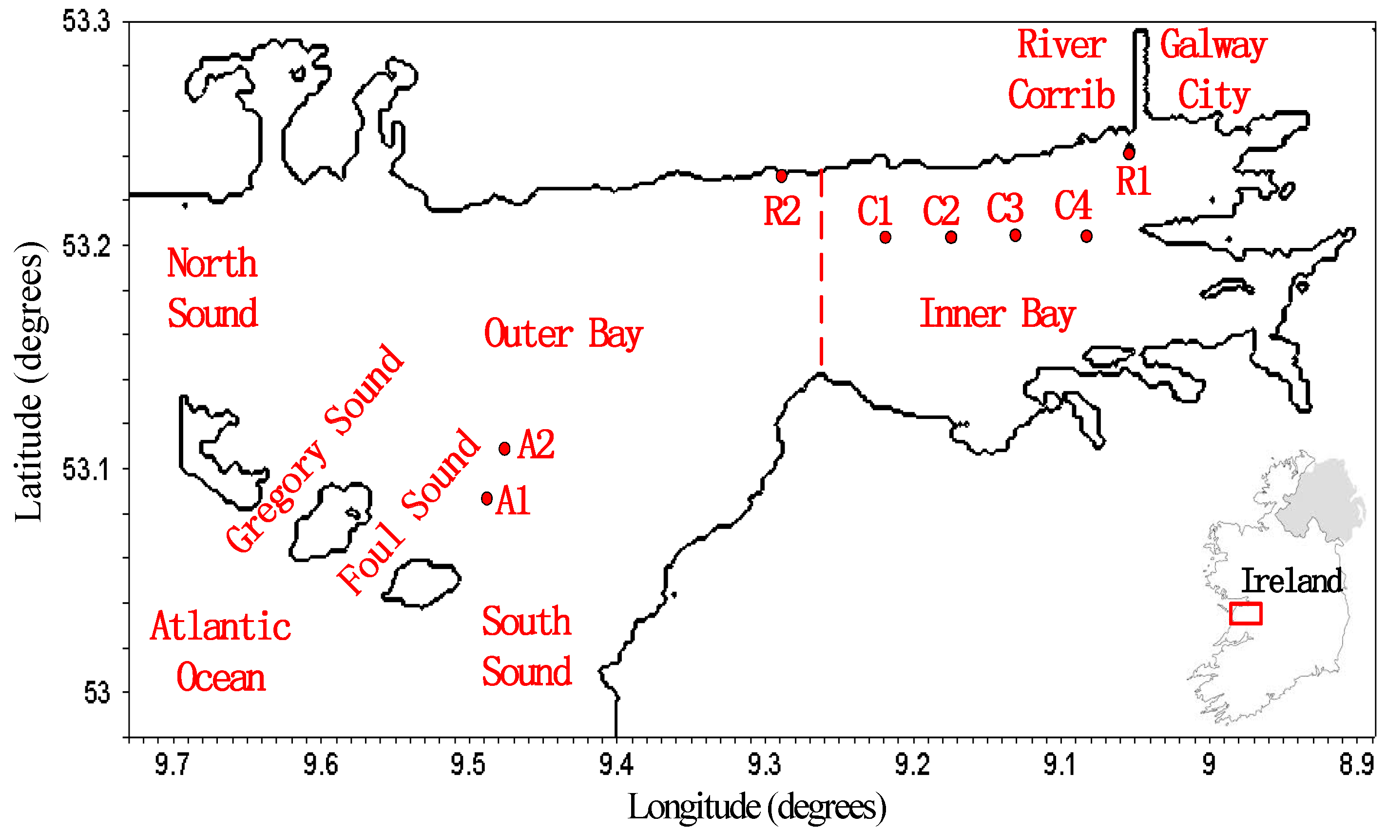
Figure 2.
Comparison between modeled HR wind data and NUIG wind data at C1. (a) Wind speed, (b) wind direction.
Figure 2.
Comparison between modeled HR wind data and NUIG wind data at C1. (a) Wind speed, (b) wind direction.

Figure 3.
P1 wind roses for (a) NUIG measured wind, and HR modeled winds at (b) C1 and (c) A2.

Figure 4.
P2 wind roses for (a) NUIG measured wind, and HR modeled winds at (b) C1 and (c) A2.

Figure 5.
P3 wind roses for (a) NUIG measured wind, and HR modeled winds at (b) C1 and (c) A2.

Figure 6.
P4 wind roses for (a) NUIG measured wind, and HR modeled winds at (b) C1 and (c) A2.

Figure 7.
Depth-averaged and surface ADCP data for (a) speed (b) direction at A2 during P1.

Figure 8.
Depth-averaged and surface ADCP data ((a) speed, (b) direction) at A2 during P2.
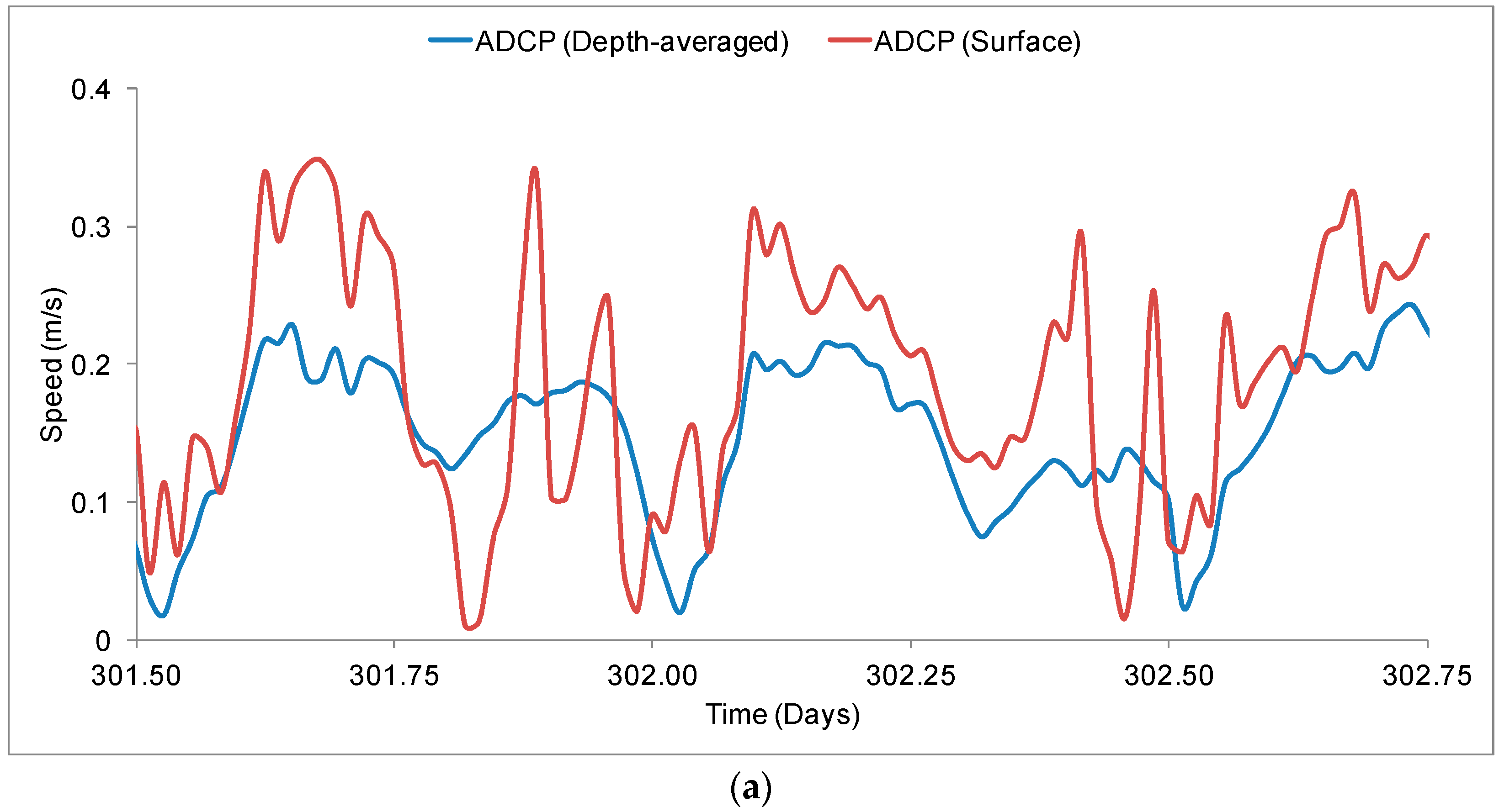

Figure 9.
Time series of HR wind at A2 against NUIG wind during P1.
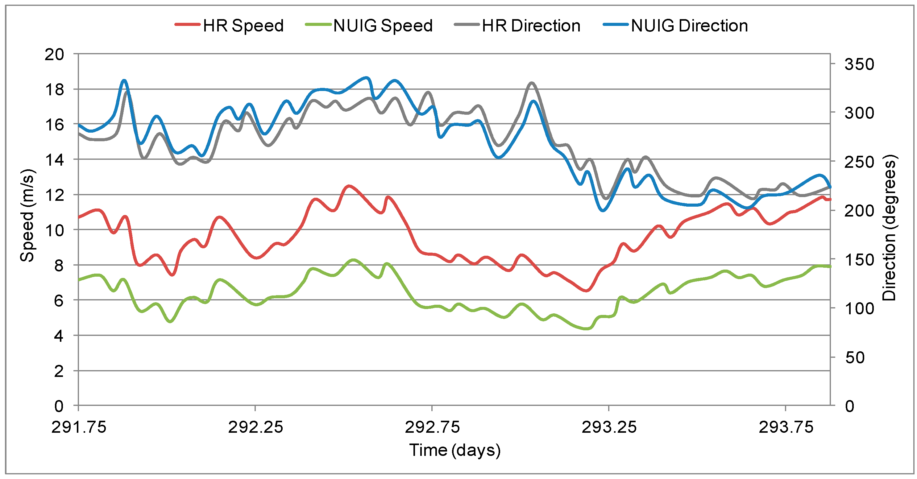
Figure 10.
Time series of HR data at A2 against NUIG wind during P2
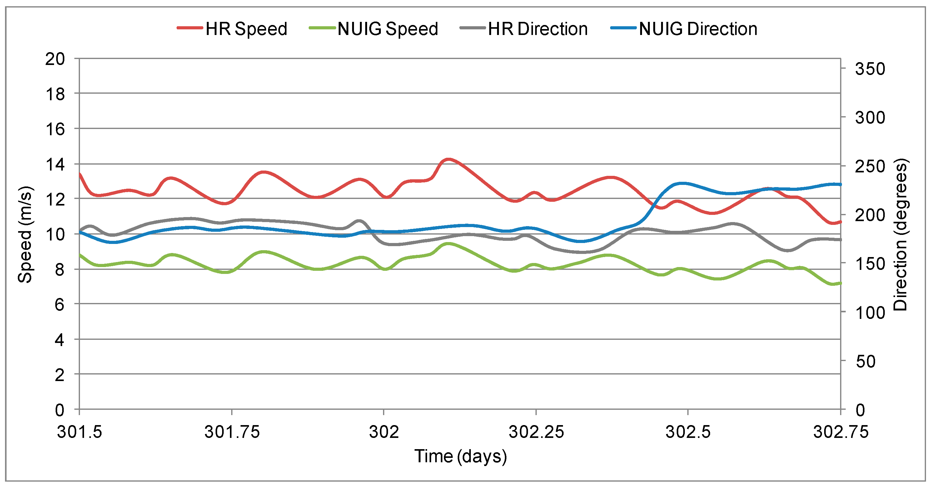
Figure 11.
(a) Sample CODAR radial vector map from Mutton Island radar station at 23:00 Julian Day 208, 201; (b) total vector map of surface currents at 15:00 Julian Day 292, 2011.
Figure 11.
(a) Sample CODAR radial vector map from Mutton Island radar station at 23:00 Julian Day 208, 201; (b) total vector map of surface currents at 15:00 Julian Day 292, 2011.

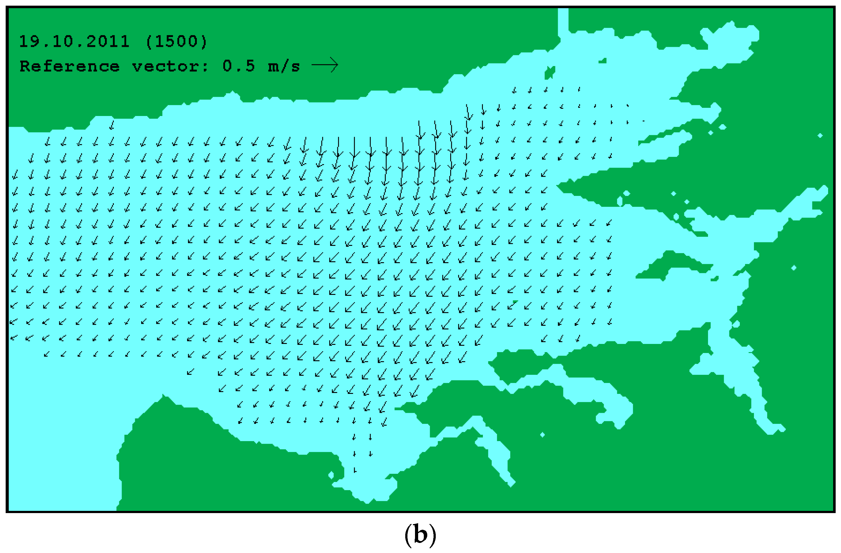
Figure 12.
Comparison of model results and observations at location C3 during P1 ((a,b) east-west (u) and north-south (v) surface velocity components from models and measurements, respectively; (c) wind speed; (d) wind direction; (e) local water elevation; (f) wind speed and wind direction at C3).
Figure 12.
Comparison of model results and observations at location C3 during P1 ((a,b) east-west (u) and north-south (v) surface velocity components from models and measurements, respectively; (c) wind speed; (d) wind direction; (e) local water elevation; (f) wind speed and wind direction at C3).
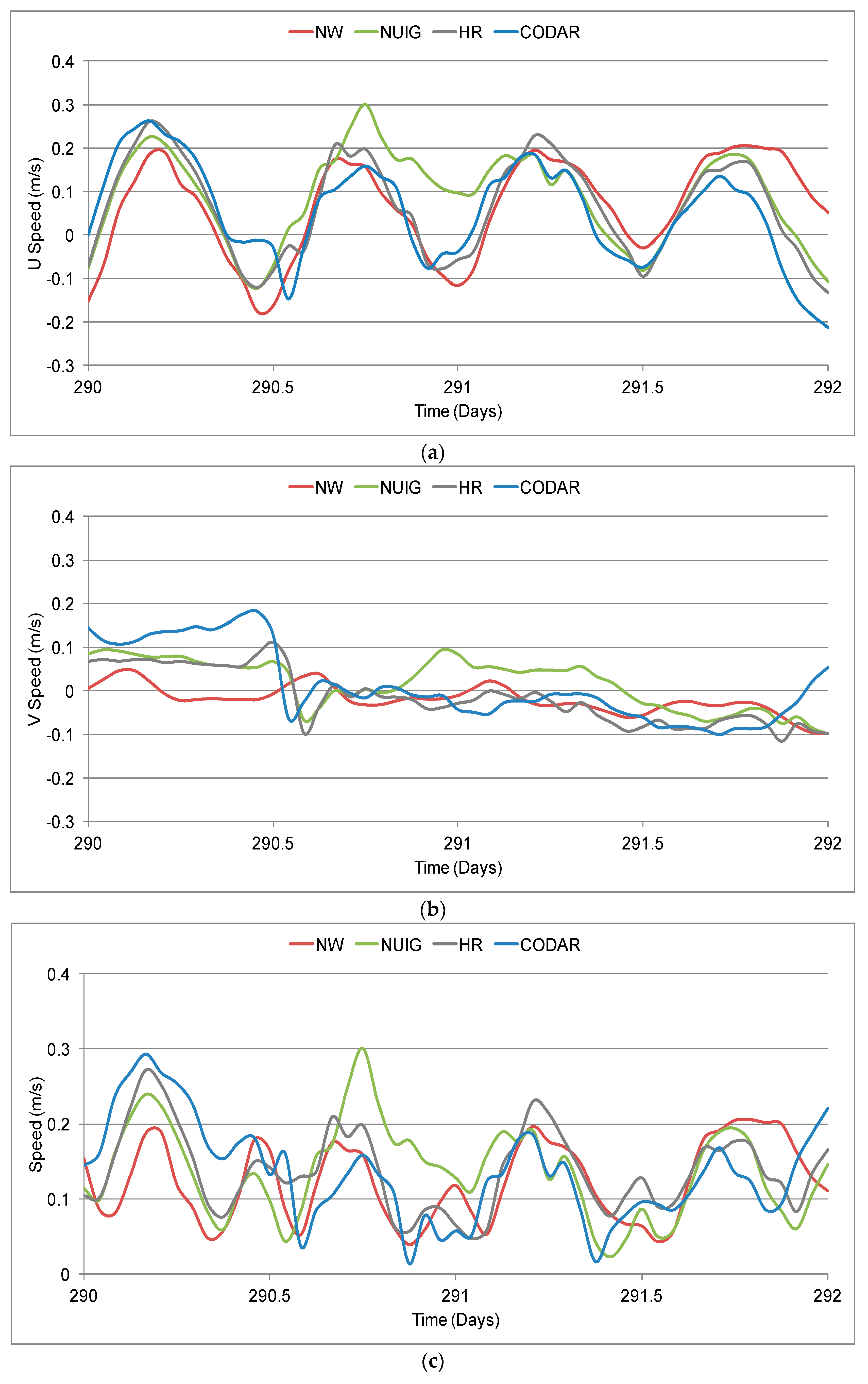

Figure 13.
Comparison of modeled and measured surface currents at locations C2 during P3 ((a), (b) east-west (u) and north-south (v) surface velocity components from models and measurements, respectively; (c) wind speed; (d) wind direction; (e) local water elevation; (f) wind speed and wind direction at C2).
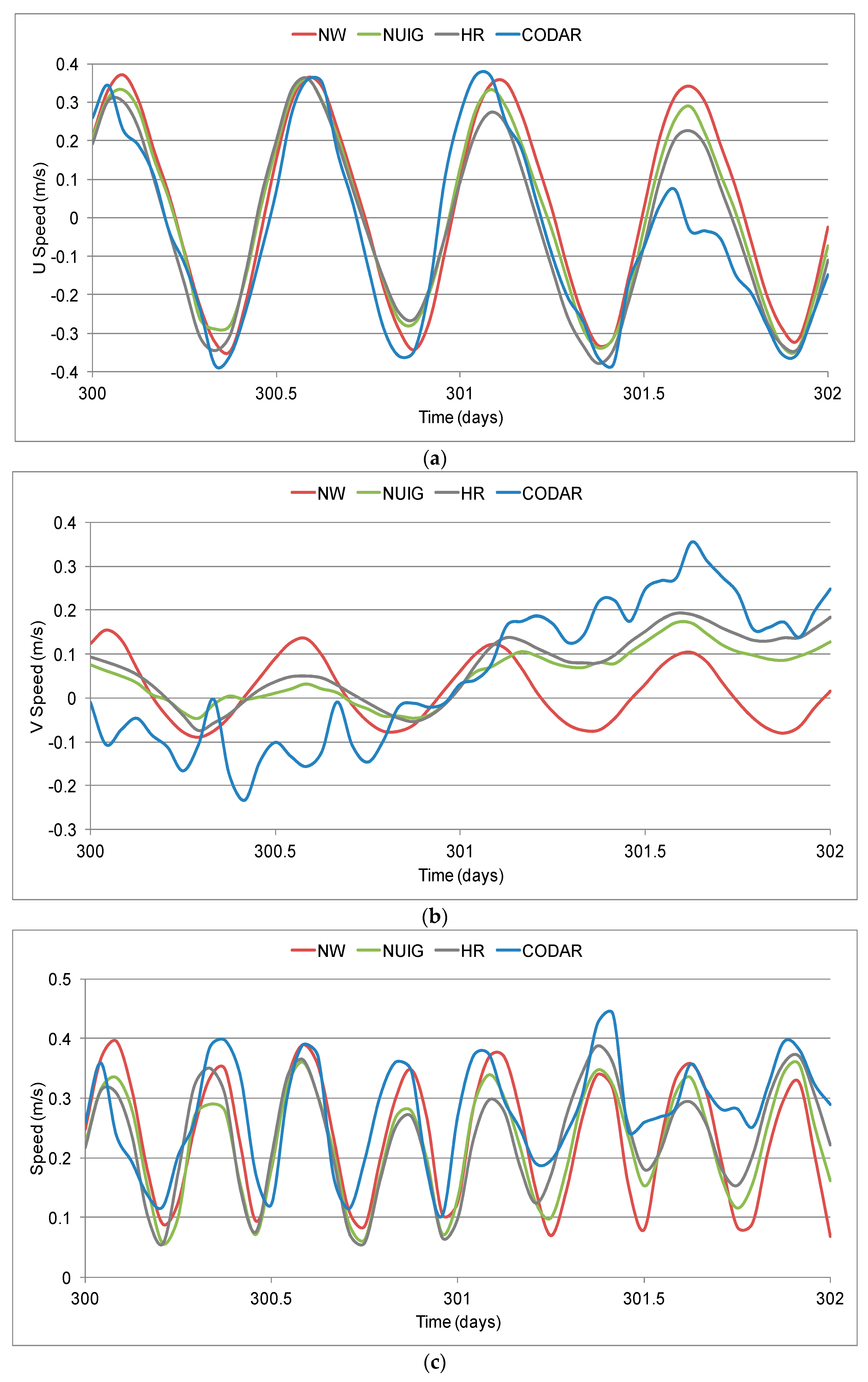

Figure 14.
(a) Water elevation curve showing times of comparison on velocity vectors and (b) HR wind speed and direction at the location C3.
Figure 14.
(a) Water elevation curve showing times of comparison on velocity vectors and (b) HR wind speed and direction at the location C3.

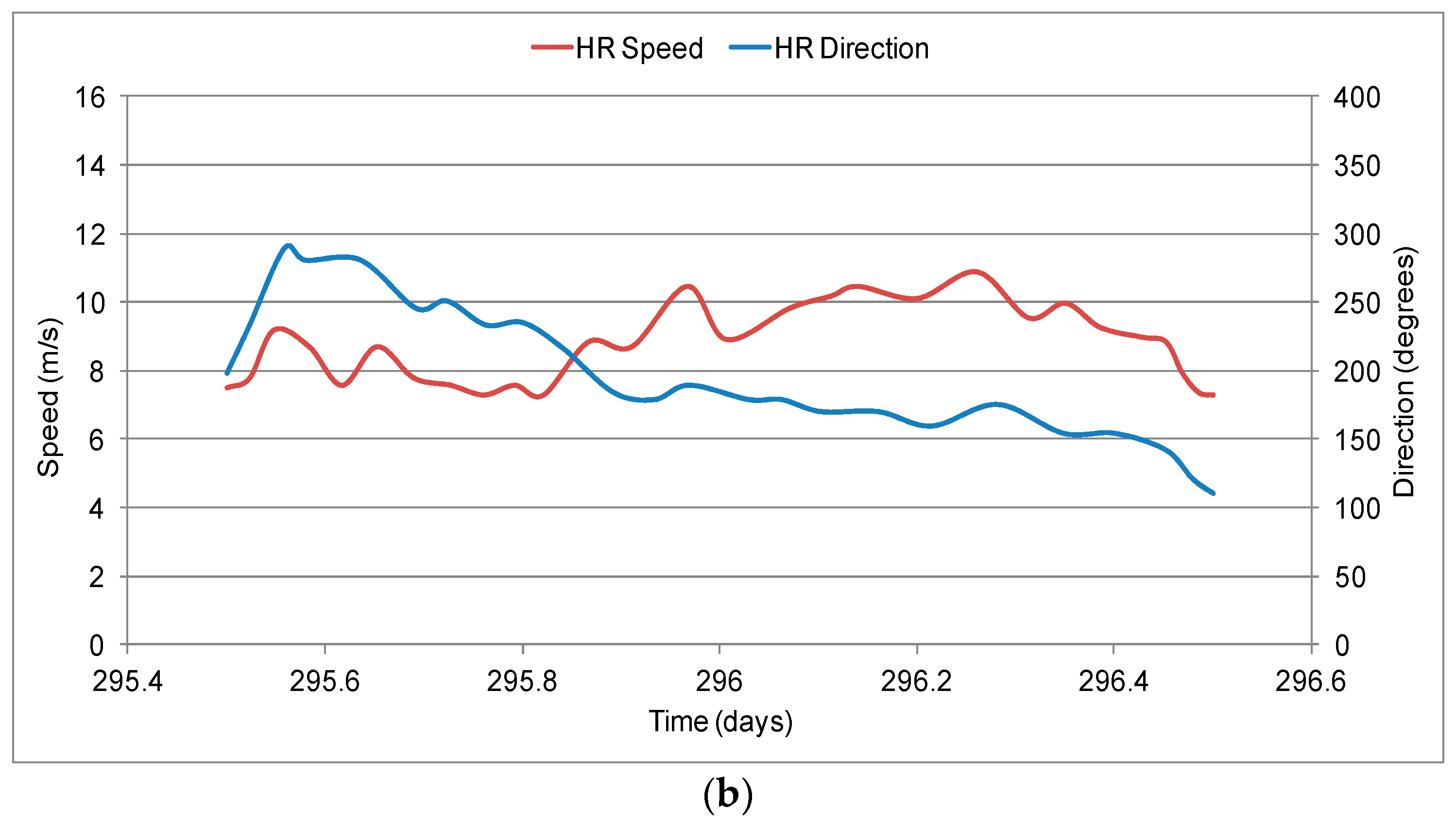
Figure 15.
Low water vector fields ((a) depth-averaged currents from model NW; (b) surface currents from model NW; (c) CODAR current data and (d) surface currents from model HR).
Figure 15.
Low water vector fields ((a) depth-averaged currents from model NW; (b) surface currents from model NW; (c) CODAR current data and (d) surface currents from model HR).
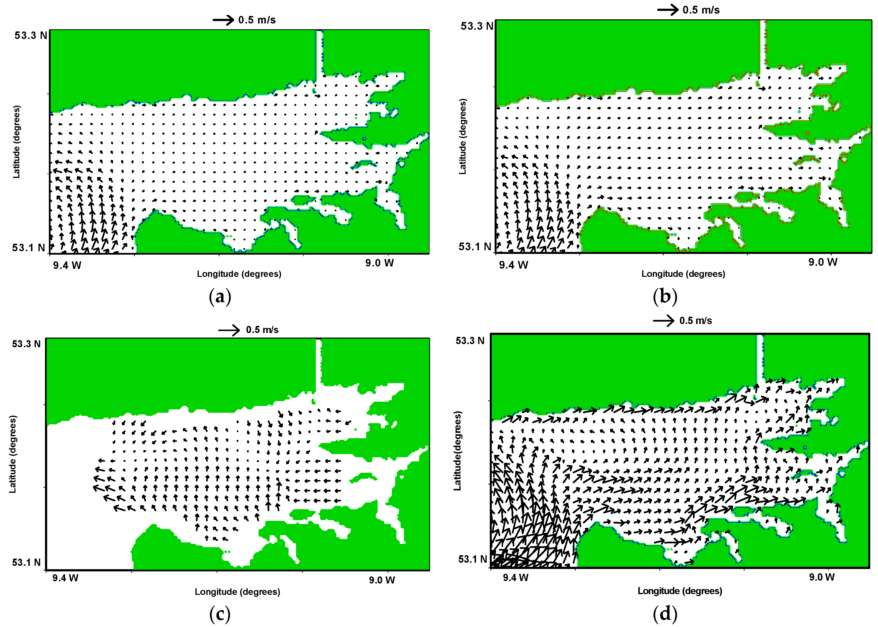
Figure 16.
Mid-flood vector fields ((a) Depth-averaged currents from model NW; (b) surface currents from model NW; (c) CODAR current data and (d) surface currents from model HR).
Figure 16.
Mid-flood vector fields ((a) Depth-averaged currents from model NW; (b) surface currents from model NW; (c) CODAR current data and (d) surface currents from model HR).

Figure 17.
High water vector fields ((a) Depth-averaged currents from model NW; (b) surface currents from model NW; (c) CODAR current data and (d) surface currents from model HR)
Figure 17.
High water vector fields ((a) Depth-averaged currents from model NW; (b) surface currents from model NW; (c) CODAR current data and (d) surface currents from model HR)

Figure 18.
Mid-ebb vector fields ((a) Depth-averaged currents from model NW; (b) surface currents from model NW; (c) CODAR current data and (d) surface currents from model HR).
Figure 18.
Mid-ebb vector fields ((a) Depth-averaged currents from model NW; (b) surface currents from model NW; (c) CODAR current data and (d) surface currents from model HR).
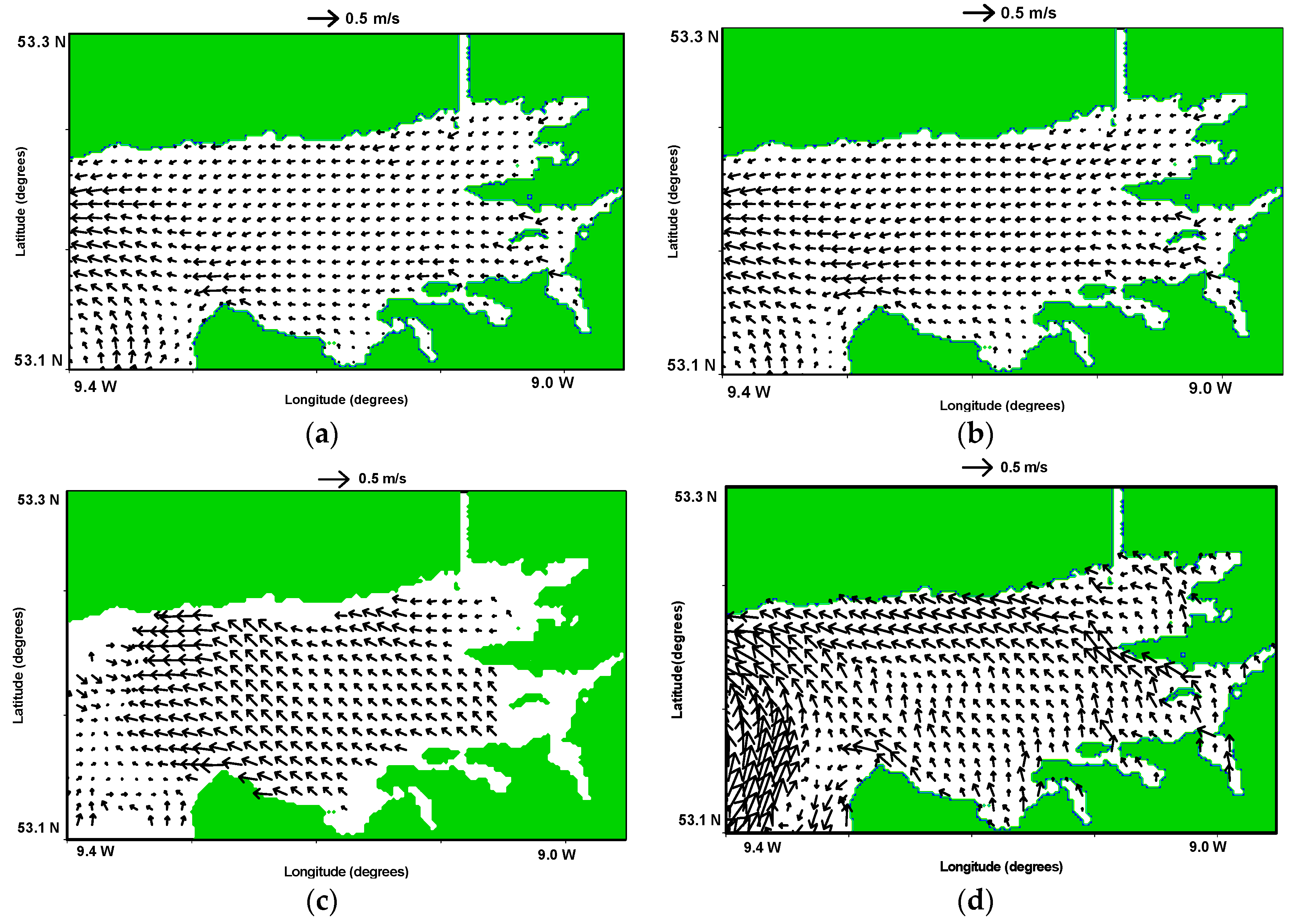
Figure 19.
Modeled and measured north-south surface velocity component at C3 ((a) north-south surface velocity components; (b) modeled wind speeds and direction at C3).
Figure 19.
Modeled and measured north-south surface velocity component at C3 ((a) north-south surface velocity components; (b) modeled wind speeds and direction at C3).


Table 1.
High resolution forecast offshore winds.
| Index | Period | Time | Duration (hours) |
|---|---|---|---|
| P1 | Period one | Julian Day 291 18:00 to Julian Day 294 00:00 | 55 |
| P2 | Period two | Julian Day 301 12:00 to Julian Day 302 17:00 | 29 |
| P3 | Period three | Julian Day 309 18:00 to Julian Day 312 00:00 | 55 |
| P4 | Period four | Julian Day 312 00:00 to Julian Day 314 06:00 | 55 |
Table 2.
Statistics of HR and NUIG wind datasets.
| Variable | Standard Deviation | Mean Difference |
|---|---|---|
| Speed (m/s) | 1.4 | 7.4 |
| Direction (°) | 18.7 | 0.9 |
Table 3.
Model scenarios.
| Model | Wind Source Used |
|---|---|
| NW | No wind forcing |
| NUIG | Temporally varying but spatially non-varying measured onshore wind |
| HR | Temporally and spatially varying offshore wind forecast offshore wind |
Table 4.
Statistics between models and CODAR.
| Period | Model | Location | RMSE (u, cm/s) | RMSE (v, cm/s) | RSQ (u) | RSQ (v) |
|---|---|---|---|---|---|---|
| P1 | NW | C3 | 11.24 | 8.63 | 0.25 | 0.08 |
| P1 | NUIG | C3 | 8.56 | 6.49 | 0.57 | 0.35 |
| P1 | HF | C3 | 5.64 | 5.57 | 0.76 | 0.66 |
| P3 | NW | C2 | 12.46 | 17.83 | 0.82 | 0.00 |
| P3 | NUIG | C2 | 9.87 | 10.95 | 0.87 | 0.74 |
| P3 | HF | C2 | 9.02 | 10.52 | 0.86 | 0.69 |
© 2017 by the authors. Licensee MDPI, Basel, Switzerland. This article is an open access article distributed under the terms and conditions of the Creative Commons Attribution (CC BY) license (http://creativecommons.org/licenses/by/4.0/).
Share and Cite
MDPI and ACS Style
Ren, L.; Nagle, D.; Hartnett, M.; Nash, S. The Effect of Wind Forcing on Modeling Coastal Circulation at a Marine Renewable Test Site. Energies 2017, 10, 2114. https://doi.org/10.3390/en10122114
AMA Style
Ren L, Nagle D, Hartnett M, Nash S. The Effect of Wind Forcing on Modeling Coastal Circulation at a Marine Renewable Test Site. Energies. 2017; 10(12):2114. https://doi.org/10.3390/en10122114
Chicago/Turabian StyleRen, Lei, Diarmuid Nagle, Michael Hartnett, and Stephen Nash. 2017. "The Effect of Wind Forcing on Modeling Coastal Circulation at a Marine Renewable Test Site" Energies 10, no. 12: 2114. https://doi.org/10.3390/en10122114
Note that from the first issue of 2016, this journal uses article numbers instead of page numbers. See further details here.