Economic Feasibility Analysis for Renewable Energy Project Using an Integrated TFN–AHP–DEA Approach on the Basis of Consumer Utility


College of Architecture and Urban-Rural Planning, Sichuan Agricultural University, Dujiangyan 611830, China
*
Author to whom correspondence should be addressed.
Energies 2017, 10(12), 2089; https://doi.org/10.3390/en10122089
Submission received: 7 October 2017
/
Revised: 14 November 2017
/
Accepted: 18 November 2017
/
Published: 9 December 2017
(This article belongs to the Special Issue Energy Efficient and Smart Cities)
Abstract
:A renewable energy (RE) project has been brought into focus in recent years. Although there is quite a lot of research to assist investors in assessing the economic feasibility of the project, because of the lack of consideration of consumer utility, the existing approaches may still cause a biased result. In order to promote further development, this study focuses on the economic feasibility analysis of the RE project on the basis of consumer utility in the whole life cycle. Therefore, an integrated approach is proposed, which consists of triangular fuzzy numbers (TFNs), an analytic hierarchy process (AHP) and data envelopment analysis (DEA). The first step is to determine the comprehensive cost index weights of DEA by TFN–AHP. Secondly, to solve the problem, the first DEA model, which is proposed by A. Charnes, W. W. Cooper and E. Rhodes (C2R), is established to calculate the DEA effectiveness. Then, the third task involves designing a computer-based intelligent interface (CBII) to simplify realistic application and ensure performance efficiency. Finally, a solar water heater case study is demonstrated to validate the effectiveness of the entire method’s system. The study shows that this could make investors’ lives easier by using the CBII scientifically, reasonably and conveniently. Moreover, the research results could be easily extended to more complex real-world applications.
1. Introduction
Recently, with the global increasing energy demand, renewable energy (RE) has emerged as a fast-growing alternative energy source to replace fossil fuels. From 2012 to 2040, the RE consumption is estimated to grow by about 2.6% a year [1]. Although it is important, the investment community still cannot fully assess and manage the underlying risk involved in this newly developing investment. The key determining factor leading to this dilemma is cost disadvantage [2]. As a result, the viability of a RE project strongly depends on the cost input. In addition, the public does not much interest in RE utilization because of the price barrier, although it will bring greater economic benefits in the long term. Thus, this makes it much more difficult for new technologies to become popular in reality.
In order to break the bottleneck of RE application, it is necessary to study the utilization cost compared with that of traditional fossil fuel energy. Consequently, some research has conducted cost analyses for different RE energies, such as solar power, wind power, hydropower, and so on [3,4,5]. Furthermore, some other scholars have studied the economic assessment of a RE system on the basis of the cost analysis [6,7,8]. Therefore, the economic feasibility has already become one of the key factors in the promotion of RE technology. However, besides the consideration of the economic benefit of investment, the public acceptance also plays an important role in project economics. In recent years, some achievements have been made in terms of consumer willingness, social acceptance, and investment willingness for RE [9,10,11,12].
Subsequently, there have been some calculation tools to assess the acceptance and willingness. Research topics such as the utilization of a linear regression model [13], a meta-regression approach [14], and a contingent valuation method [10,15] have often been studied. Because the public acceptance of RE is hugely dependent on people’s subjective judgment, a lack of consideration of the consumer’s behavior rule will lead to a biased result in research. Thus, the theory of consumer utility can help to solve the problem more reasonably and efficiently. However, few scholarly works have put forward such a solution approach based on the utility theory. With the higher demand of RE application, the focus of traditional study foci has shifted to consumer behavior in reality. Therefore, assuring the promotion of the RE project is very important.
The rapid development of RE technologies with unmatched hysteresis brings many new challenges. This study investigates how these challenges can be overcome by a computer-based intelligent interface (CBII), which supports an integrated triangular funny number–analytic hierarchy process–data envelopment analysis (TFN–AHP–DEA) approach, as well as how to evaluate economic feasibility of the RE project on the basis of consumer utility in the whole life cycle. Specifically, this paper proposes a DEA model with the corresponding cost index, input and output parameters. Then, the comprehensive index weights are determined by an AHP with TFNs. Furthermore, the first DEA model, which is proposed by A. Charnes, W. W. Cooper and E. Rhodes (C2R), is the classical mode of DEA, is used to evaluate the technical efficiency and scale efficiency of decision making units (DMUs) by using linear programming [16]. In order to solve the problem, a model is established to calculate the DEA effectiveness. In order to implement the approach more simply and conveniently, a CBII is designed. Finally, the initial cost, benchmark cost, adjusted cost and incremental cost are analyzed further to provide useful advice for different decision makers.
This study contributes to the literature by improving the economic feasibility assessment of the RE project through the consideration of consumer utility in the whole life cycle. The proposed novel approach enhances the traditional study foci and improves the existing methodologies. To ensure convenience in practical applications, an understandable CBII can help researchers and practitioners more expediently with a scientific and effective implementation.
This paper is organized as follows. Firstly, the background of the study is given in Section 2. Secondly, the integrated TFN–AHP–DEA model is proposed in Section 3. Thirdly, the design and implementation of the CBII are outlined in Section 4. Fourthly, Section 5 analyzes two case studies of solar water heater utilization in the Chinese Panxi region and Yunnan-Guizhou Plateau. Finally, the advantages, limitations, and possible future extensions of this work are discussed in Section 6.
2. Background of the Study
The global energy crisis requires the rapid development of the RE industry to be relieved. However, the cost disadvantage and price barrier impede the implementation process of the new technologies. In this situation, it is very important for the RE project to assess the cost analysis and economic feasibility.
2.1. The Related Literature
In recent years, some scholars have paid more attention to the cost analysis of RE technologies. Atsu et al. [3] state that solar photovoltaic generation has the potential to become cost-effective in the future. As parallel results, Wiser et al. [4] studied the potential benefits of wind energy’s sustainable development. Aghahosseini et al. [5] propose a techno-economic study of an entirely renewable energy-based power supply including solar power, wind power, hydropower and other main energy sources. The evaluation of economic feasibility on the basis of cost analysis has attracted many foci accordingly. Ortega and Río [6] studied the economic benefit through the cost of renewable electricity in Europe. Akikur et al. [7] explored the economic feasibility of solar energy and a solid oxide fuel cell-based cogeneration system in Malaysia. Moreover, Park [8] explored the economic feasibility of using renewable electricity generation systems.
Additionally, the public acceptance has also directly impacted RE popularization. Štreimikienė and Baležentis [9] assessed the willingness to pay for RE technologies in Lithuania. Park et al. [10] analyzed the feasibility of RE implementation by considering Korean customers' willingness to pay. Further, Solangi et al. [11] studied the social acceptance of solar energy in Malaysia from the users’ perspective. Particularly, Xu [12] researched the willingness to invest in a building that uses integrated photovoltaics and is grid-connected. Meanwhile, some useful calculation tools, which are used to estimate acceptance and willingness level, have been studied. Hast et al. [13] analyzed consumers’ willingness to pay for a RE system using generalized linear regression models. Sundt and Rehdanz [14] present a meta-regression to explain the differences in the willingness to pay for RE products. Park et al. [10] and Lee and Heo [15] explored the contingent valuation method to estimate the willingness to pay for RE technologies.
However, because of the subjective judgment in people’s willingness and acceptance of RE consumption, this may bring biased results in assessments. Thus, the theory of consumer utility can help to solve the problem more reasonably and efficiently.
2.2. Method Description
This paper explores the economic feasibility of the RE project on the basis of consumer utility in the whole life cycle. The novel approach consists of TFNs, AHP and DEA, which can deal with the proposed research issues and orient the realistic problems.
The evaluation theory of TFNs is based on fuzzy theory, which was put forward by Zadeh in 1965 and has been applied to quality management and risk management [17]. Baloi and Price [18] have pointed out that fuzzy logic theory provides a useful way to deal with ill-defined and complex problems in a decision-making environment. Therefore, the evaluation method is more suitable to describe the subjective decision according to the people’s thinking mode in the discussed problem.
Saaty [19] proposed an AHP, which is a simple and flexible decision-making method for dealing with both qualitative and quantitative judgments [20,21]. The main advantages of using the AHP methodology are the following: (1) The definition of the hierarchical structure in AHP can help us to explain all the complex relationships. (2) The method integrates all the judgments with the structured links [22]. Consequently, this paper combines some basic TFN theory [23] with AHP to calculate the comprehensive consumer acceptable level.
The traditional cost analysis methods include the net present value model, the dynamic payback period model and the cost-benefit analysis (CBA). The CBA model is a widely used pre-assessment tool. However, it has caused considerable controversy in converting soft variables (e.g., quality) into money, or excluding qualitative variables directly from the outside analysis [24]. At the same time, it may not take the costs and benefits, which reflect views from people of different groups, into account [25]. Yang et al. [26] demonstrated that the existing studies in CBA focus mostly on calculating the cost of projects, while the proportion of their benefits remains small. Furthermore, Liu and Mi [26] state that the existing life-cycle cost (LCC) analysis methods lack reliable cost-effectiveness assessments for energy-efficient projects. Meanwhile, ignoring the uncertain data used in LCC analysis is a distinct problem. This will cause inaccurate results [27]. Although sensitivity analysis can be applied in cost projects, this method puts more focus on the importance and influence of the factors [28]. The common cost analysis methods generally require function expression and database normalization. Furthermore, most scholars usually analyze from the perspective of investors, but there is little consideration of the consumer’s utility to analyze the cost of the project.
DEA, which was put forward by Charnes et al. [29], is used to evaluate the efficiency of DMUs with complex production relationships [30]. In fact, it has been used to perform the comparison analysis, sensitivity analysis and efficiency analysis between the target value and actual value [31]. In the DEA model, it is not necessary to know the model’s structure for the variables’ relationship [30]. In particular, it has also been applied to compare the efficiency of projects [32]. Above all, it is suitable to measure the performance of similar units in a multi-input and -output project.
However, it is insufficient to consider other units in the traditional DEA model; thus the evaluation is subjective [30]. In the traditional model, the input and output values are known, but the observed data are imprecise in practical applications. It may not reflect the overall distribution of the data [33,34]. Therefore, it is necessary to improve this method by combining it with TFN–AHP, as in this study.
The proposed method can be utilized to solve the economic assessments of renewable energy projects. The superiorities of the TFN–AHP–DEA approach are as follows:
- (1)
- Because of the different influences of the input and output values, the proposed method utilizes the AHP to calculate the weights.
- (2)
- The traditional AHP method uses a lack of linguistic variables; thus the proposed method can avoid information distortion by combining TFNs with the AHP method.
- (3)
- The common cost analysis methods generally require function expression and database normalization, while the DEA method does not have to take these into consideration. Additionally, most scholars have been studying cost analysis from the investor’s perspective rather than from the consumer’s perspective. The DEA method is significant for the consumers’ decision. It is utilized in the comparison analysis, sensitivity analysis and efficiency analysis.
- (4)
- The conventional DEA model can only process precise data. To reflect decision-makers’ subjective judgments, the TFN–AHP–DEA method can calculate fuzzy data, which is obtained by specialists.
Therefore, in this study, an integrated TFN–AHP–DEA approach is provided to calculate the comprehensive consumer acceptable level with complex fuzzy data on the basis of the consumer utility in the whole life cycle.
2.3. Proposed Research Framework
Above all, a framework of economic feasibility analysis on the basis of consumer utility for the RE project is expressed in Figure 1 and includes three research phases given by the following:
Phase I: This describes the theories and methods that are used to build the model. Furthermore, the input and output parameters in the model are determined through the identifying of the model elements.
Phase II: To achieve the case analysis, the model and intelligent tool are implemented on the basis of the original data; then the results of the TFN–AHP–DEA model are analyzed and discussed.
Phase III: To express the technical route in this paper, this is divided into eight steps. The most important step is to compare the initial cost, benchmark cost, adjusted cost and incremental cost.
Phase IV: The conclusion and suggestion are received in the end of this research.
3. TFN–AHP–DEA Approach
3.1. Approach Preparation
The DEA system uses the input and output parameters to implement a comprehensive analysis of the initial cost, benchmark cost, adjusted cost and incremental cost.
Input: Index of consumption cost in the whole life cycle. According to the literature and research, the purchase cost, renewal fee and maintenance charge are considered as the inputs.
Output: Index of customer acceptable level. Through consulting the literature [35,36], this mainly depends on the economic efficiency, functional character and comfortable capability of the RE product.
Initial cost: The sum of all the initial inputs.
Benchmark cost: The cost to obtain hot water without the utilization of a solar water heater, including electricity, liquefied gas and firewood mode.
Adjusted cost: The sum of all the adjusted inputs.
Incremental cost: The difference value between the adjusted cost and benchmark cost.
3.2. Consumer Acceptable Level Calculation
In this study, the customer utility is mainly expressed through the customer acceptance level. The calculated comprehensive acceptable level can be categorized as the DMUs in TFN–AHP–DEA.
3.2.1. Index Weight Determination
The index weights are determined by using TFN–AHP [19,23] in this paper. The details are presented as below.
Judgment matrix: According to the comparison scale in Table 1, on the basis of the investigated respondent’s answer, the judgment matrix is shown in Equation (1):
Here, is a reciprocal matrix; , and ; that is to say, .
Consistency checking: If for all and the matrix is a consistency judgment matrix, then the triangular fuzzy judgment matrix is a consistent fuzzy judgment matrix [38]. The calculation process is as below [18]:
Here, is the eigenvector, and is the maximum eigenvalue of the matrix ; is the number of criteria compared in matrix [19].
Here, is the consistency index, is the consistency ratio, and is the average random consistency index. It is acceptable when [39].
Important degree: According to the fuzzy matrix, the comprehensive important level of each element is calculated as follows [23]:
Probability chance: Calculating the probability of each index being greater than others is as shown in Equation (10) [23]:
The probability between two triangular fuzzy numbers is as shown below in Equation (11) [23]:
Weight matrix: Through the normalization processing of the above, , the weight matrix is obtained as in Equation (12):
Here,
3.2.2. Comprehensive Acceptable Level Calculation
Through combining the qualitative and quantitative methods, the acceptance levels are defined. Thus, completely unacceptable is 1 point, unacceptable is 3 points, acceptable is 5 points, more acceptable is 7 points, completely acceptable is 9 points, and in the middle are 2, 4, 6, and 8.
The questionnaire survey was used to obtain the acceptable level of the consumers in different modes. Then, combining this with the weight calculated by TFN–AHP, the comprehensive acceptable level is obtained using Equation (13):
According to the calculated comprehensive acceptable level of each consumer, except for the acceptable level below 5 points, the others can be categorized as the DMUs in the TFN–AHP–DEA approach.
3.3. DEA Model Building
3.3.1. C2R Model
This paper adopts the C2R model with a non-Archimedean infinitesimal epsilon in Equation (14):
Here, is the relative efficiency score; is a non-Archimedean infinitesimal number; and are the slack variable and the surplus variable, respectively; is the optimum value; is the involvement of input by DMUn; is the produce of output by DMUn; and is used to judge the return to scale of DMU.
3.3.2. Ineffective Decision-Making Unit Transformation
According to the calculation of Equation (14), the effective and ineffective DMUs are determined by judging as in Equation (15):
The ineffective DMU is adjusted to an effective DMU as in Equation (16) below [40]:
Here , and are the optimal solutions of the linear programming corresponding to the DMU. is the projection that on the relative effective surface corresponds to the previous DMU .
3.3.3. Adjusted Cost Calculation
According to Equation (16), the adjusted cost is calculated as in Equation (17):
3.3.4 Incremental Cost Calculation
According to Equation (17), the incremental cost is calculated as in Equation below (18):
Here represents the benchmark cost of the -th.
From the above, through the proposed integrated TFN–AHP–DEA approach, the incremental cost values can be obtained when the traditional energy is converted into RE energy. Furthermore, it can help project investors to judge the economic feasibility on the basis of customer utility in the whole life cycle.
4. CBII Design
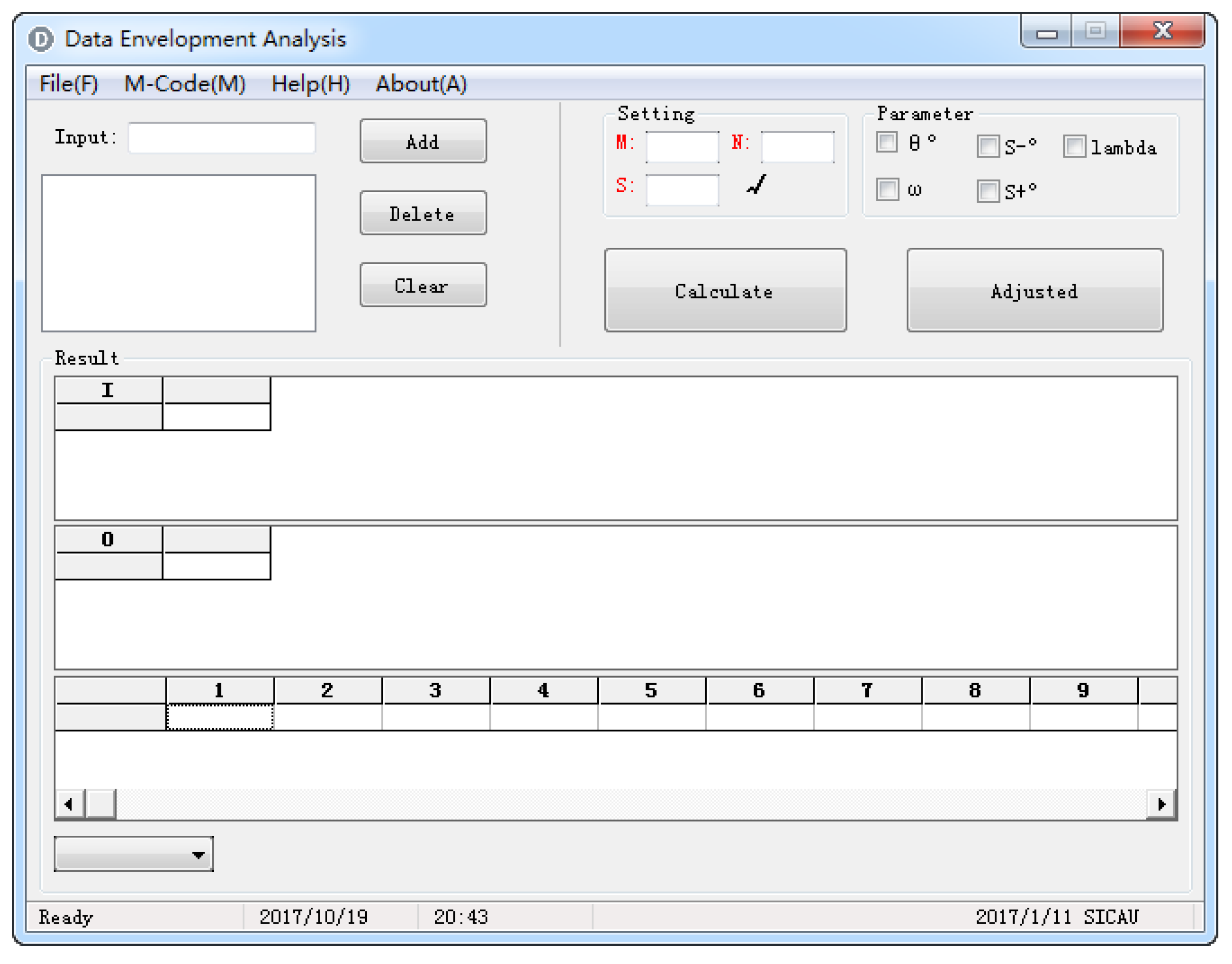
In order to make the proposed approach implementation simpler and more convenient, a CBII is designed. The interface system, which is designed by visual basic 6.0 and MATLAB 8.3 (released in 2014, adding local modeling to the single precision design), mainly consists of three parts: data import, a relative effectiveness calculation and an ineffective DMU adjustment. The integrated interface is shown in Figure 2.
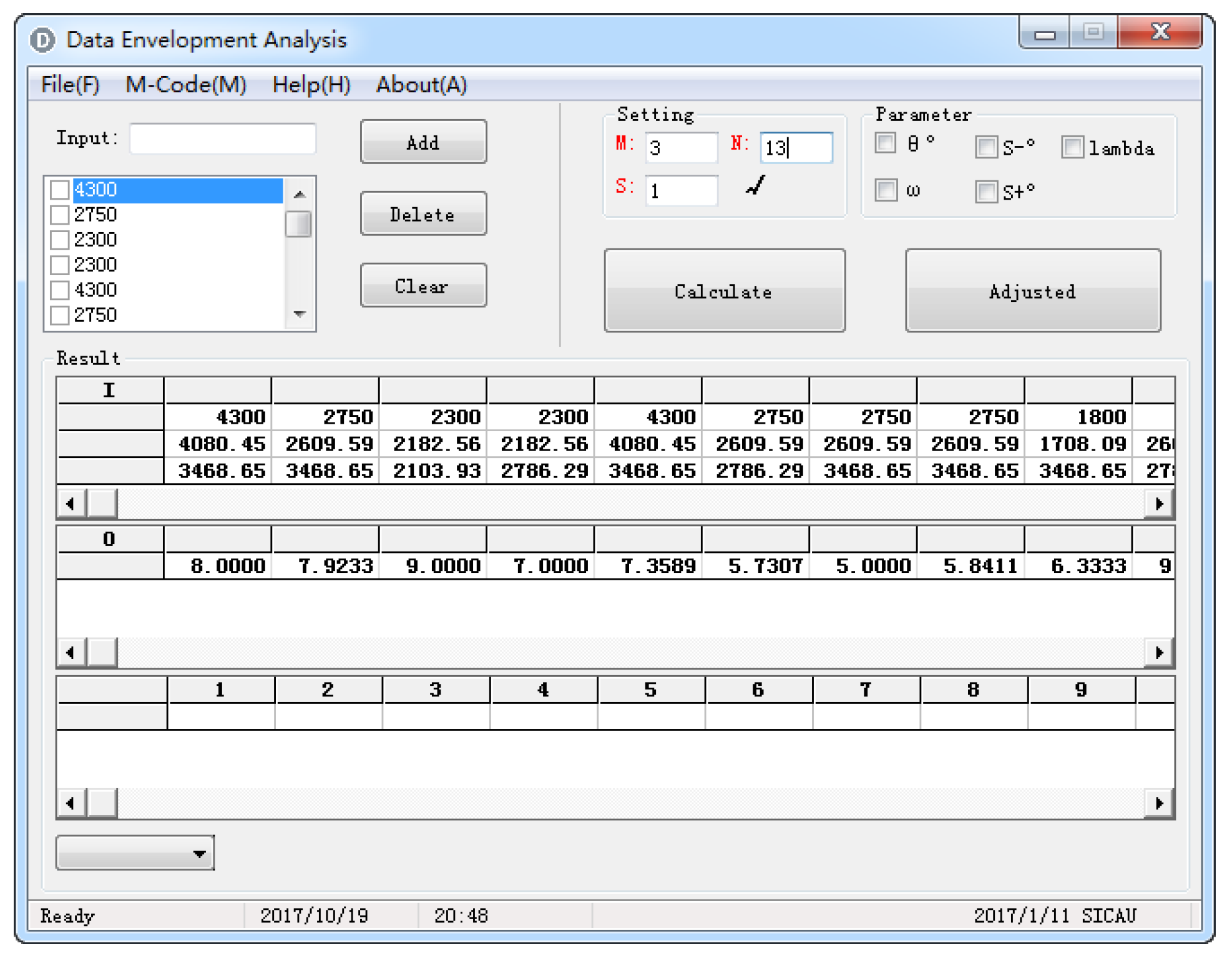
4.1. Data Import
After the system parameters , and have been set in the interface of the CBII, the input and output data can be directly imported into the system, as shown in Figure 2. Here, M represents the number of inputs in the C2R model, is the number of DMUs in the C2R model, and is the number of outputs in the C2R model. Consequently, and appear in the result.
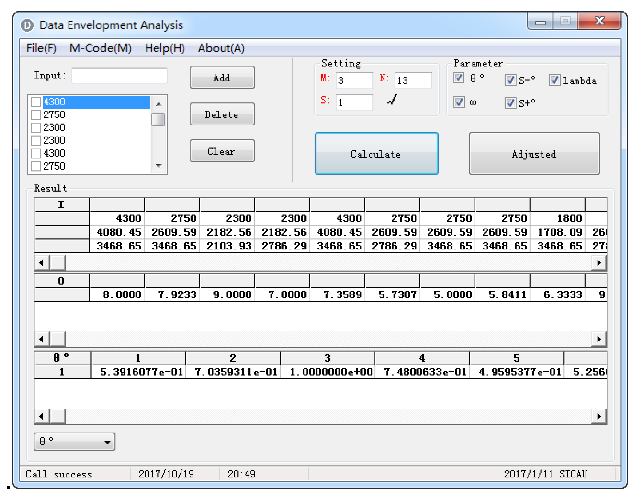
4.2. Relative Effectiveness Calculation
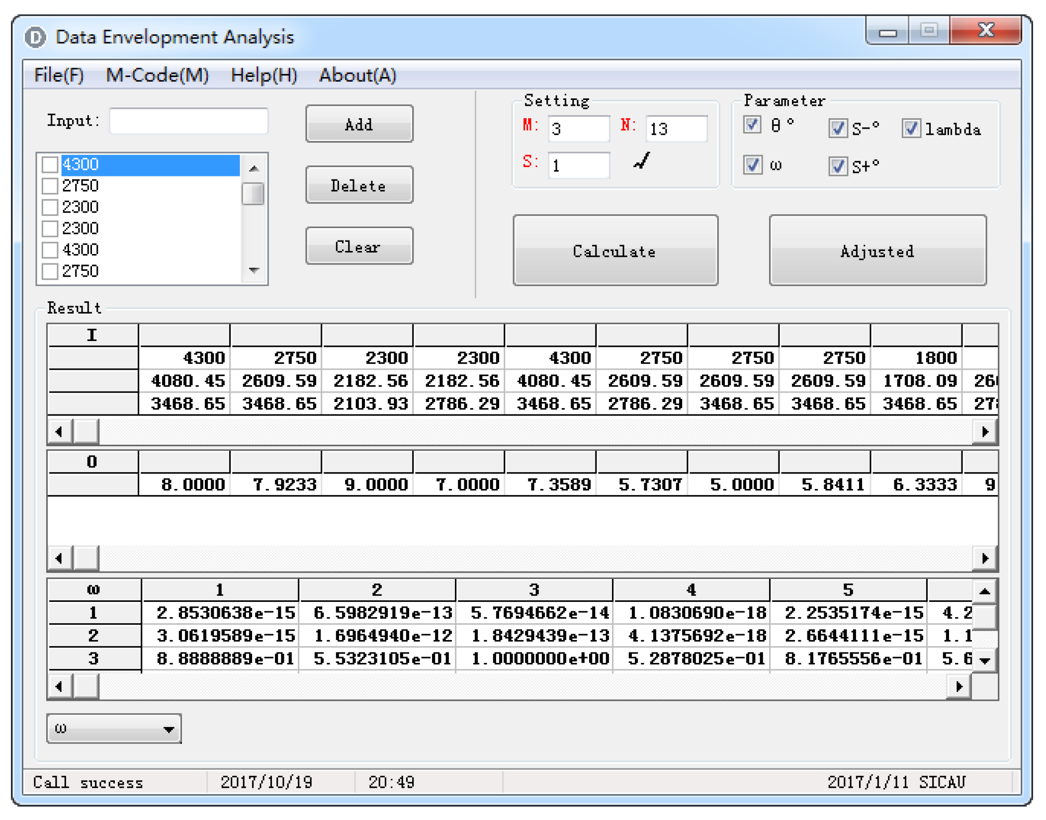
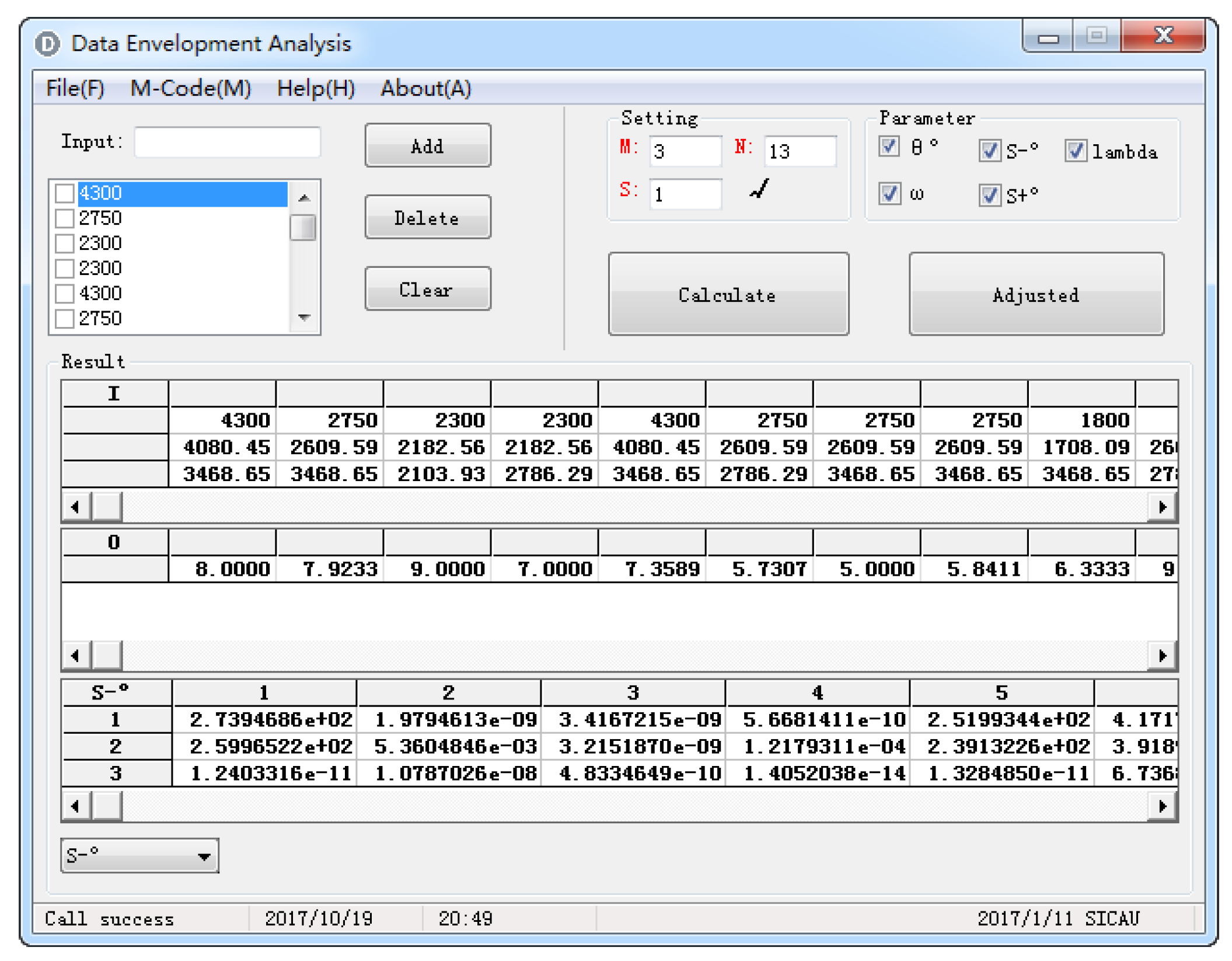
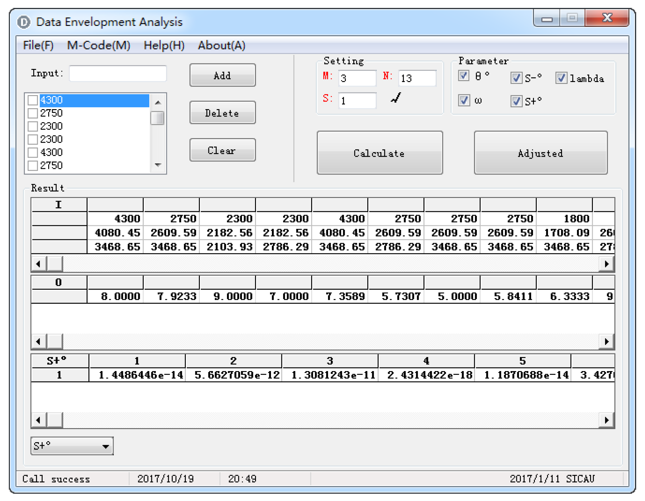
There are five parameters in the C2R model, , , , and lambda. Here lambda represents the weight coefficient, which is used to judge the return to scale of DMU. After clicking “Calculate” in the interface, the calculation is completed.
4.3. The Adjustment of Ineffective Decision-Making Unit
According to Equation (11) in Section 3, only one of the parameters , or can be chosen at this step. For example, after selecting the parameter, we need select , or in the drop-down list, and then click “Adjust”; then the adjusted I and O are received.
5. Case Study
5.1. Input and Output Data Collection
This paper takes the energy saving technology of a solar water heater as the research object and the Chinese Panxi region as case study 1. In order to verify the serviceability of the proposed method, this paper takes the Yunnan-Guizhou Plateau as case study 2. Both of these have the same RE resources in different regions with a similar climate.
Through the investigation and application of the TFN–AHP method, as introduced previously, the output is obtained (here, , and are directly obtained through surveys). is calculated by Equations (1), (3), and (7)–(13). However, the input should be processed further, as follows:
Here is the initial purchase cost. and are the minimum and the maximum unit prices for purchasing a solar water heater, respectively. It is accepted by the survey.
Here represents the updating fee considering the time value of money [41], = 0.35% is the annual interest rate, e represents the update times, and t is the useful life of the solar water heater. Here, this value is 15 years.
Here represents the use of maintenance fee. Similarly, it considers the time value of money [41]. is the present value. is the annual value, that is, the reinvestment cost each year. represents the housing service life period. It is assumed that the housing service life period in rural regions is 30 years, while in urban regions it is 50 years.
and represent the charges for maintenance and usage. According to the survey, all values are considered as 50 yuan, and of using firewood is not considered; is the conversion coefficient, as shown in Table 2; is the unit price and is the kettle capacity. According to the survey, takes a value of 10 L; is the resident population; represents the number of times in a year that the solar water heater cannot be used for 3–5 continuous days. This is calculated by the data from the weather website.
5.1.1. Case Study 1
There are total of 34 valid questionnaires from urban and rural areas, respectively. The data from the Panxi region is shown in Table 3.
According to the data in Table 3, there are 14, 13 and 7 DMUs for the different energy modes applied into the DEA. However, the units with comprehensive consumer acceptable level below 5 should be abandoned according to this study. Thus, 13, 12 and 6 DMUs for different energy modes were finally applied into TFN–AHP–DEA method, respectively.
5.1.2. Case Study 2
There are total of 33 valid questionnaires from urban and rural areas, respectively. The data from the Yunnan-Guizhou Plateau region is shown in Table 4.
According to the data in Table 3, there are 19, 10 and 4 DMUs for the different energy modes applied into the DEA. However, the units with comprehensive consumer acceptable level below 5 should be abandoned according to this study. Thus, 16, 8 and 4 DMUs for the different energy modes were finally applied into the TFN–AHP–DEA method, respectively.
5.2. Case Implementation
5.2.1. Case Study 1
Through the implementation of the case data from the Panxi region in the CBII, the relative effectiveness of each DMU of the different energy modes was calculated. Then the ineffective DMU was adjusted to be effective, and the initial cost, benchmark cost, adjusted cost and incremental cost were calculated. The summary data is shown in Table 5. The italic numbers represent the results of the traditional DEA. The bold numbers represent the results of the TFN–AHP–DEA method.
5.2.2. Case Study 2
The data from the Yunnan-Guizhou Plateau region was processed in the same way. The summary data is shown in Table 6. The italic numbers represent the results of the traditional DEA. The bold numbers represent the results of the TFN–AHP–DEA method.
5.2.3. CBII Implementation Process
5.3. Result Analysis
According to the data in Table 5 and Table 6, the initial cost, benchmark cost, adjusted cost and incremental cost of using electricity, liquefied gas and firewood are analyzed. Thus, the average incremental cost of the unit area on the basis of the consumer acceptable level in the Panxi region and Yunnan-Guizhou Plateau region are presented in Table 7.
As shown in Table 7, the following can be clearly obtained: (1) The average incremental cost of using firewood is positive. However, the average incremental cost of using liquefied gas and electricity are negative. This indicates that a household’s consumption, which previously used liquefied gas and electricity, can be decreased in the whole life cycle by using an alternative solar water heater, while the families using firewood will face a more incremental cost. (2) Furthermore, the total weighted incremental cost of the unit area is negative. This demonstrates that using a solar water heater can bring economic benefits to the whole life cycle.
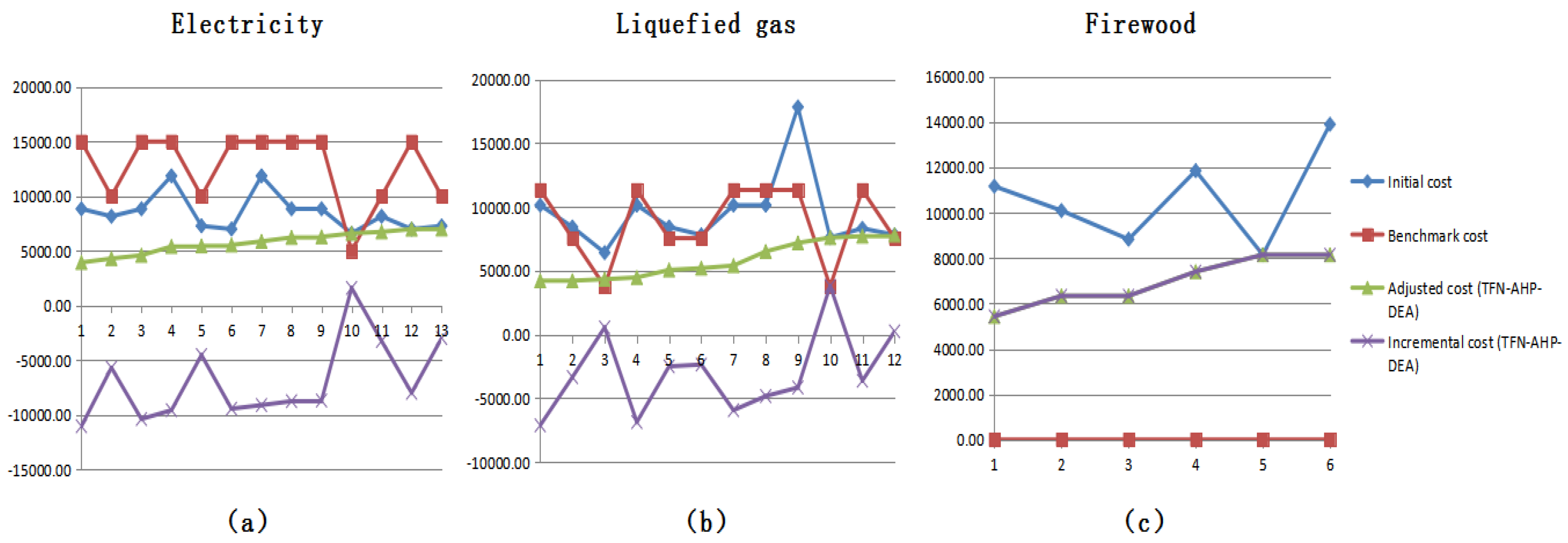
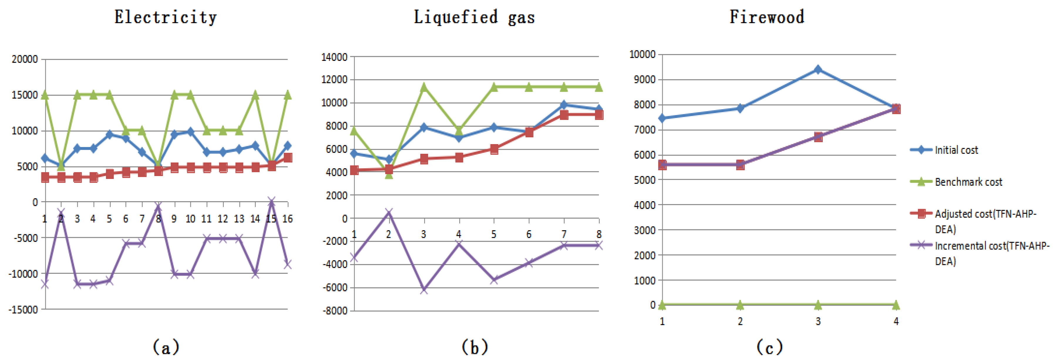
In addition, the changes and relationships of the initial cost, benchmark cost, adjusted cost and incremental cost in different energy modes are shown in Figure 11 and Figure 12. In both figures, the horizontal represents the different survey objects and the vertical represents the price of the initial cost, benchmark cost, adjusted cost and incremental cost in different energy modes. In addition, we use the data from Table 5 and Table 6 in Figure 11, Figure 12, Figure 13 and Figure 14.
The results of the incremental cost analysis are consistent on the whole; the stability and availability of this model is proved. From Figure 11 and Figure 12, it can be seen that the adjusted cost is clearly lower than the initial cost. Thus, although the benchmark cost is high, the incremental cost is almost negative in Figure 11a,b and Figure 12a,b. This indicates that if a customer chooses a solar water heater instead of using electricity and liquefied gas, they can receive economic benefits. However, because the cost of using firewood is very low, the benchmark cost is ignored in this paper. Consequently, the incremental cost is equal to the adjusted cost in Figure 11c and Figure 12c. Although these users might face an incremental cost, this customer group has few people and would only have a little influence on promoting RE.
Furthermore, a comparison of traditional DEA and the proposed TFN–AHP–DEA approach has been presented to show the advantages, as shown in Figure 13 and Figure 14.
From both the figures, the results of traditional DEA show that the incremental cost is higher than the results with the TFN–AHP–DEA approach on the basis of customer utility. Therefore, although the first approach is easier to implement, the calculation results still need to be improved.
Above all, case studies 1 and 2 illustrate that if the cost is controlled and optimized reasonably, economic benefits can be obtained and the purpose of RE popularization can be achieved in different regions. This means that the proposed TFN–AHP–DEA approach is applicable to the same RE resources in different regions with a similar climate.
6. Conclusions
This research identifies the economic influence factors that will promote RE technologies. Under the consideration of customer utility in the whole life cycle, the economic feasibility of the RE project can be analyzed and evaluated more reasonably. This study provides a novel integrated TFN–AHP–DEA approach to deal with the problem. It also designs a CBII as a useful tool to make the approach implementation simpler and more convenient. There are five main advances in the paper: Firstly, the adjusted cost is clearly lower than the initial cost, which is an advantage for RE promotion. Secondly, through a comprehensive analysis of the initial cost, benchmark cost, adjusted cost and incremental cost, it can be seen that using a solar water heater can bring direct economic benefits. This shows that the RE projects have great promotional significance. Thirdly, the application of the proposed approach can be used to evaluate the consumer acceptable level from a cost perspective and thus to promote the use of RE. Furthermore, the effectiveness of the TFN–AHP–DEA approach should be distinguished from that of the traditional DEA; it proves its superiority in this paper. Finally, more significantly, the designed CBII is tested to be feasible in different regions, making it simple and convenient for investors and consumers. Therefore, this study finds it has potential to promote the RE technology through cost reduction.
However, there still exist worthy further research prospects in three areas: (1) Exploring the economic feasibility of other RE technologies in the case of consumer acceptance. (2) Taking into account the boundary condition of the RE technology and the corresponding environment benefits under the condition of consumer acceptance. (3) Applying the approach and the CBII tool into more areas. Each aspect of further research is of great significance to the promotion of the RE project.
Acknowledgments
This work was supported by the Humanities Social and Sciences Research Funds of Education Ministry (Grant No. 15XJC630001), the Key Funds of Sichuan Social Science Research Institution “System Science and Enterprise Development Research” (Grant No. Xq15B09), and the Youth Funds of Sichuan Provincial Education Department (Grant No. 14ZB0014).
Author Contributions
Lu Gan conceived the framework, developed the models and wrote the majority of the paper; Dirong Xu designed the algorithm, performed the experiments and presented the results; Lin Hu integrated the data and performed the development of the paper; Lei Wang designed the computer-based intelligent interface.
Conflicts of Interest
The authors declare no conflict of interest.
References
- Sharma, R.; Goel, S. Performance evaluation of stand alone, grid connected and hybrid renewable energy systems for rural application: A comparative review. Renew. Sustain. Energy Rev. 2017, 78, 1378–1389. [Google Scholar]
- Chang, C.Y. A critical analysis of recent advances in the techniques for the evaluation of renewable energy projects. Int. J. Proj. Manag. 2013, 31, 1057–1067. [Google Scholar] [CrossRef]
- Atsu, D.; Agyemang, E.O.; Tsike, S.A.K. Solar electricity development and policy support in Ghana. Renew. Sustain. Energy Rev. 2016, 53, 792–800. [Google Scholar] [CrossRef]
- Wiser, R.; Bolinger, M.; Heath, G.; Keyser, D.; Lantz, E.; Macknick, J.; Millstein, D. Long-term implications of sustained wind power growth in the United States: Potential benefits and secondary impacts. Appl. Energy 2016, 179, 146–158. [Google Scholar] [CrossRef]
- Aghahosseini, A.; Bogdanov, D.; Breyer, C. A Techno-Economic Study of an Entirely Renewable Energy-Based Power Supply for North America for 2030 Conditions. Energies 2017, 10, 1171. [Google Scholar] [CrossRef]
- Ortegaizquierdo, M.; Río, P.D.; Kazmerski, L. Benefits and costs of renewable electricity in Europe. Renew. Sustain. Energy Rev. 2016, 61, 372–383. [Google Scholar] [CrossRef]
- Akikur, R.K.; Saidur, R.; Ullah, K.R.; Hajimolana, S.A.; Ping, H.W.; Hussain, M.A. Economic feasibility analysis of a solar energy and solid oxide fuel cell-based cogeneration system in Malaysia. Clean Technol. Environ. Policy 2016, 18, 669–687. [Google Scholar] [CrossRef]
- Park, E. Potentiality of renewable resources: Economic feasibility perspectives in South Korea. Renew. Sustain. Energy Rev. 2017, 79, 61–70. [Google Scholar] [CrossRef]
- Štreimikienė, D.; Baležentis, A. Assessment of willingness to pay for renewables in Lithuanian households. Clean Technol. Environ. Policy 2015, 17, 515–531. [Google Scholar] [CrossRef]
- Park, S.H.; Jung, W.J.; Kim, T.H.; Lee, S.Y.T. Can Renewable Energy Replace Nuclear Power in Korea? An Economic Valuation Analysis. Nucl. Eng. Technol. 2016, 48, 559–571. [Google Scholar] [CrossRef]
- Solangi, K.H.; Saidur, R.; Luhur, M.R.; Aman, M.M.; Badarudin, A.; Kazi, S.N.; Islam, M.R. Social acceptance of solar energy in Malaysia: Users’ perspective. Clean Technol. Environ. Policy 2015, 17, 1975–1986. [Google Scholar] [CrossRef]
- Xu, R. The restriction research for urban area building integrated grid-connected PV power generation potential. Energy 2016, 113, 124–143. [Google Scholar]
- Hast, A.; Alimohammadisagvand, B.; Syri, S. Consumer attitudes towards renewable energy in China—The case of Shanghai. Sustain. Cities Soc. 2015, 17, 69–79. [Google Scholar] [CrossRef]
- Sundt, S.; Rehdanz, K. Consumers’ willingness to pay for green electricity: A meta-analysis of the literature. Energy Econ. 2015, 51, 1–8. [Google Scholar] [CrossRef]
- Lee, C.Y.; Heo, H. Estimating willingness to pay for renewable energy in South Korea using the contingent valuation method. Energy Policy 2016, 94, 150–156. [Google Scholar] [CrossRef]
- Otay, I.; Oztaysi, B.; Onar, S.C.; Kahraman, C. Multi-expert performance evaluation of healthcare institutions using an integrated intuitionistic fuzzy AHP&DEA methodology. Knowl.-Based Syst. 2017, 133, 90–106. [Google Scholar]
- Zadeh, L.A. Fuzzy sets. Inf. Control 1965, 8, 338–353. [Google Scholar] [CrossRef]
- Baloi, D.; Price, A.D.F. Modelling global risk factors affecting construction cost performance. Int. J. Proj. Manag. 2003, 21, 261–269. [Google Scholar] [CrossRef]
- Saaty, T.L. The Analytic Hierarchy Process: Planning, Priority Setting, Resource Allocation; McGraw-Hill: New York, NY, USA, 1980. [Google Scholar]
- Kahraman, C.; Cebeci, U.; Da, R. Multi-attribute comparison of catering service companies using fuzzy AHP: The case of Turkey. Int. J. Prod. Econ. 2004, 87, 171–184. [Google Scholar] [CrossRef]
- Macharis, C.; Springael, J. PROMETHEE and AHP: The design of operational synergies in multicriteria analysis: Strengthening PROMETHEE with ideas of AHP. Eur. J. Oper. Res. 2004, 153, 307–317. [Google Scholar] [CrossRef]
- Bertolini, M.; Braglia, M.; Carmignani, G. Application of the AHP methodology in making a proposal for a public work contract. Int. J. Proj. Manag. 2006, 24, 422–430. [Google Scholar] [CrossRef]
- Veerabathiran, R.; Srinath, K.A. Application of the extent analysis method on fuzzy AHP. Int. J. Eng. Sci. Technol. 2012, 4, 3472–3480. [Google Scholar]
- Beukers, E.; Bertolini, L.; Brömmelstroet, M.T. Why Cost Benefit Analysis is perceived as a problematic tool for assessment of transport plans: A process perspective. Transp. Res. Part A 2012, 46, 68–78. [Google Scholar] [CrossRef]
- Martens, K. Substance precedes methodology: On cost–benefit analysis and equity. Transportation 2011, 38, 959–974. [Google Scholar] [CrossRef] [Green Version]
- Yang, X.; Teng, F.; Xi, X.; Khayrullin, E.; Zhang, Q. Cost–benefit analysis of China’s Intended Nationally Determined Contributions based on carbon marginal cost curves. Appl. Energy 2017, in press. [Google Scholar] [CrossRef]
- Giuseppe, E.D.; Iannaccone, M.; Telloni, M.; D’Orazio, M.; di Perna, C. Probabilistic life cycle costing of existing buildings retrofit interventions towards nZE target: Methodology and application example. Energy Build. 2017, 144, 416–432. [Google Scholar] [CrossRef]
- Martin, R.; Lazakis, I.; Barbouchi, S.; Johanning, L. Sensitivity analysis of offshore wind farm operation and maintenance cost and availability. Renew. Energy 2016, 85, 1226–1236. [Google Scholar] [CrossRef] [Green Version]
- Charnes, A.; Cooper, W.W.; Rhodes, E. Measuring the efficiency of decision making units. Eur. J. Oper. Res. 1979, 2, 429–444. [Google Scholar] [CrossRef]
- Han, Y.; Long, C.; Geng, Z.; Zhang, K. Carbon emission analysis and evaluation of industrial departments in China: An improved environmental DEA cross model based on information entropy. J. Environ. Manag. 2017, 205, 298. [Google Scholar] [CrossRef]
- Podinovski, V.V. Bridging the gap between the constant and variable returns-to-scale models: Selective proportionality in data envelopment analysis. J. Oper. Res. Soc. 2004, 55, 265–276. [Google Scholar] [CrossRef]
- Vitner, G.; Rozenes, S.; Spraggett, S. Using data envelope analysis to compare project efficiency in a multi-project environment. Int. J. Proj. Manag. 2006, 24, 323–329. [Google Scholar] [CrossRef]
- Shiraz, R.K.; Fukuyama, H.; Tavana, M.; di Caprio, D. An integrated data envelopment analysis and free disposal hull framework for cost-efficiency measurement using rough sets. Appl. Soft Comput. 2016, 46, 204–219. [Google Scholar] [CrossRef]
- Geng, X.; Qiu, H.; Gong, X. An extended 2-tuple linguistic DEA for solving MAGDM problems considering the influence relationships among attributes. Comput. Ind. Eng. 2017, 112, 135–146. [Google Scholar] [CrossRef]
- Chau, C.K.; Tse, M.S.; Chung, K.Y. A choice experiment to estimate the effect of green experience on preferences and willingness-to-pay for green building attributes. Build. Environ. 2010, 45, 2553–2561. [Google Scholar] [CrossRef]
- Mell, I.C.; Henneberry, J.; Hehl-Lange, S.; Keskin, B. To green or not to green: Establishing the economic value of green infrastructure investments in The Wicker, Sheffield. Urban For. Urban Green. 2016, 18, 257–267. [Google Scholar] [CrossRef]
- Zhou, X.G.; Gao, X.D. Method of selection construction projects based on FANP model and its application. Syst. Eng.-Theory Pract. 2012, 32, 2459–2466. [Google Scholar]
- Zhao, W. Extension and Application of AHP. Math. Pract. Theory 1997, 27, 165–180. [Google Scholar]
- Si, S.K.; Sun, Z.L.; Sun, X.J. Mathematical Modeling Algorithm and Application; National Defense Industrial Press: Beijing, China, 2015. [Google Scholar]
- Ma, Z.X. Data Envelopment Analysis Model and Method; Science Press: Beijing, China, 2010. [Google Scholar]
- Liu, X.J. Engineering Economics; China Architecture & Building Press: Beijing, China, 2008. [Google Scholar]
Figure 1.
The framework of this research.
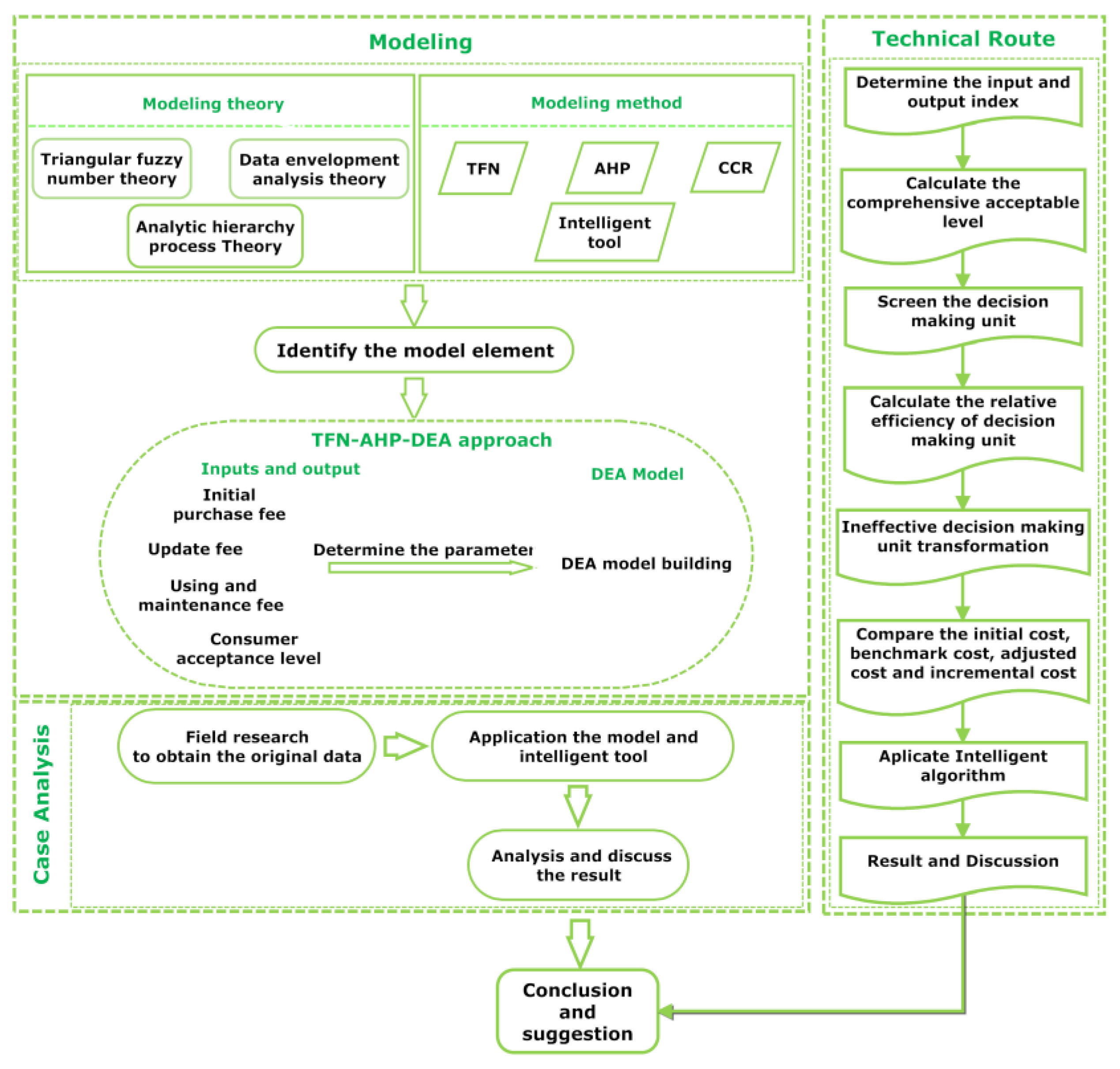
Figure 2.
The integrated interface of computer-based intelligent interface (CBII).

Figure 3.
Setting the system parameters , and .

Figure 4.
Selecting and calculating the model parameters.
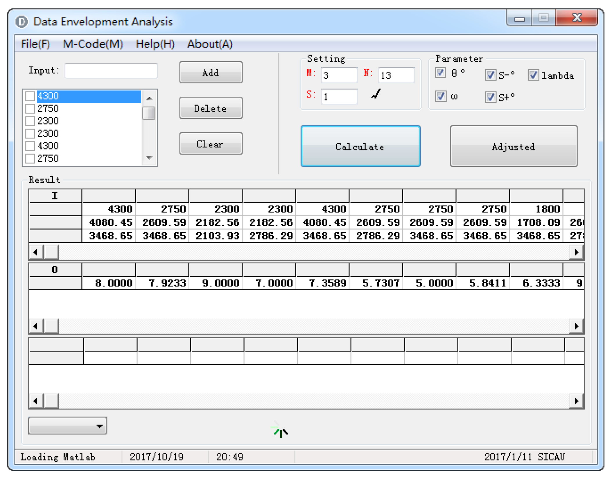
Figure 5.
The calculation result with parameter .

Figure 6.
The calculation result with parameter .

Figure 7.
The calculation result with parameter .

Figure 8.
The calculation result with parameter .

Figure 9.
The calculation result with parameter lambda. Here lambda represents the weight coefficient, which is used to judge the return to scale of DMU.
Figure 9.
The calculation result with parameter lambda. Here lambda represents the weight coefficient, which is used to judge the return to scale of DMU.
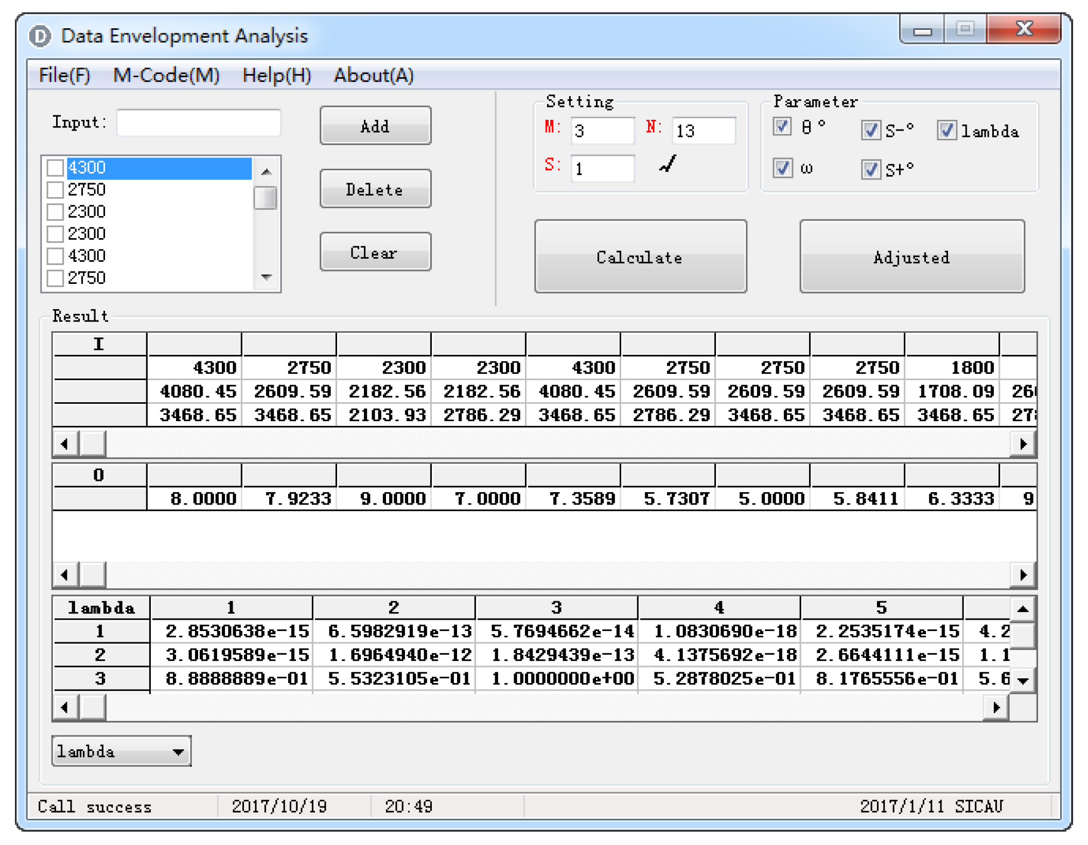
Figure 10.
The adjusted calculation results.
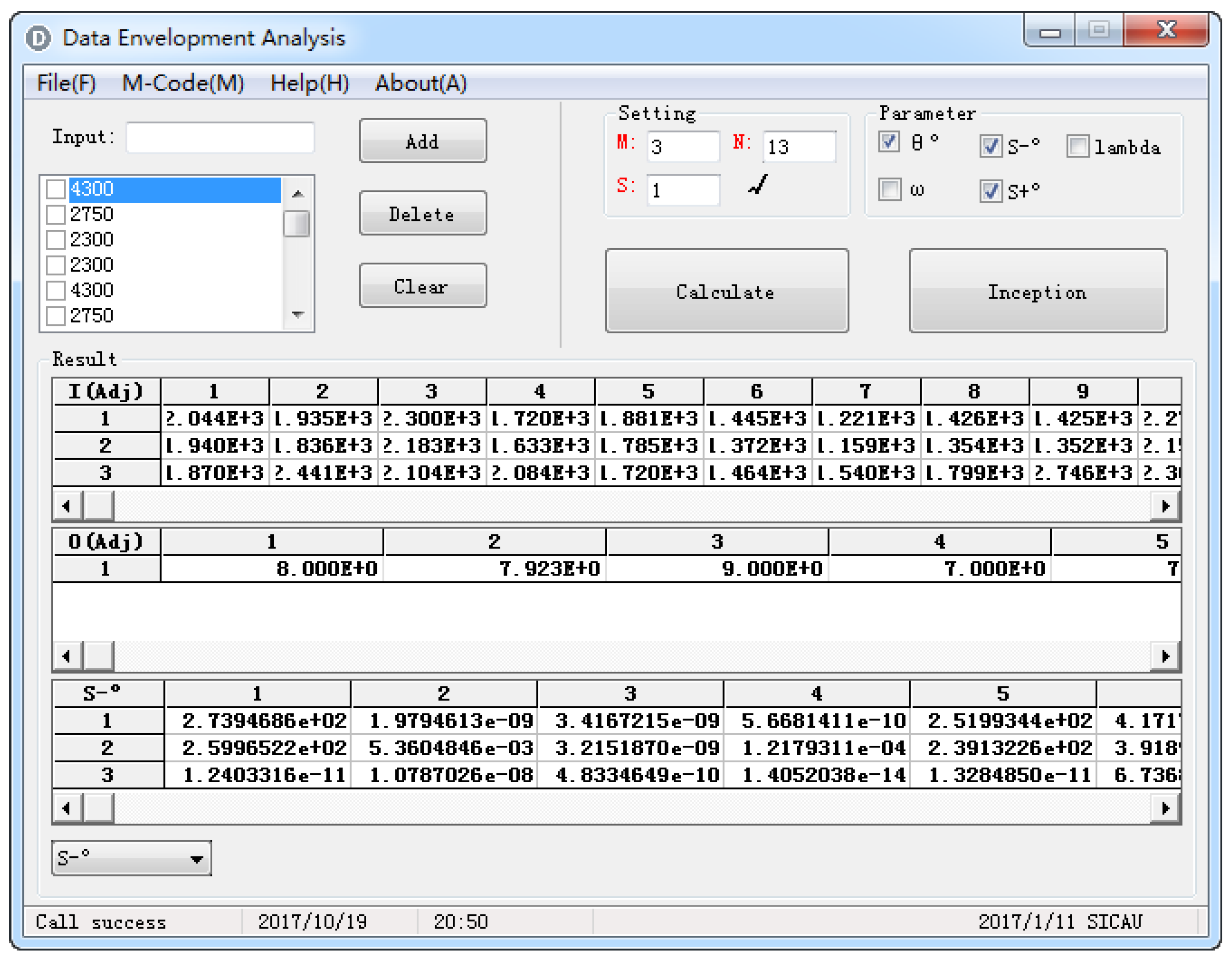
Figure 11.
The changes and relationships of initial cost, benchmark cost, adjusted cost and incremental cost in different energy modes using triangular fuzzy number–analytic hierarchy process–data envelopment analysis (TFN–AHP–DEA) approach in case study 1: (a) means the electricity; (b) means the liquefied gas; (c) means the firewood.

Figure 12.
The changes and relationships of initial cost, benchmark cost, adjusted cost and incremental cost in different energy modes using triangular fuzzy number–analytic hierarchy process–data envelopment analysis (TFN–AHP–DEA) approach in case study 2: (a) means the electricity; (b) means the liquefied gas; (c) means the firewood.

Figure 13.
The comparison of adjusted cost and incremental cost in different energy modes using data envelopment analysis (DEA) and triangular fuzzy number–analytic hierarchy process–DEA (TFN–AHP–DEA) in case study 1: (a) means the electricity; (b) means the liquefied gas; (c) means the firewood.
Figure 13.
The comparison of adjusted cost and incremental cost in different energy modes using data envelopment analysis (DEA) and triangular fuzzy number–analytic hierarchy process–DEA (TFN–AHP–DEA) in case study 1: (a) means the electricity; (b) means the liquefied gas; (c) means the firewood.
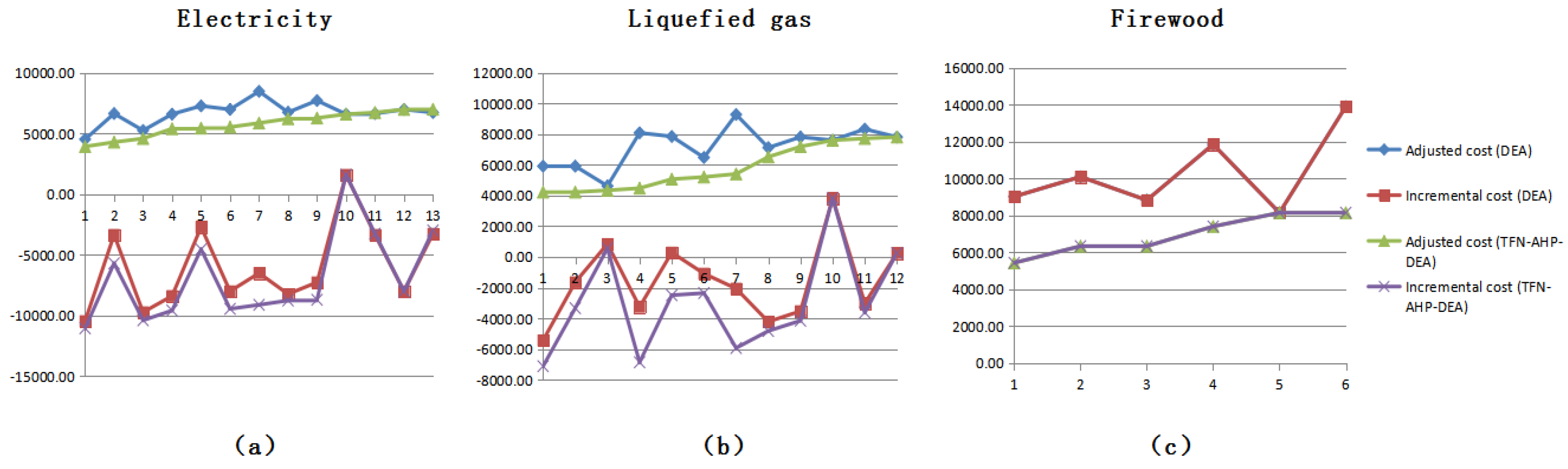
Figure 14.
The comparison of adjusted cost and incremental cost in different energy modes using data envelopment analysis (DEA) and triangular fuzzy number–analytic hierarchy process–DEA (TFN–AHP–DEA) in case study 2: (a) means the electricity; (b) means the liquefied gas; (c) means the firewood.
Figure 14.
The comparison of adjusted cost and incremental cost in different energy modes using data envelopment analysis (DEA) and triangular fuzzy number–analytic hierarchy process–DEA (TFN–AHP–DEA) in case study 2: (a) means the electricity; (b) means the liquefied gas; (c) means the firewood.


Table 1.
Linguistic variables based on triangular fuzzy numbers (TFNs).
| Linguistic Variable | TFN | The Reciprocal of TFN |
|---|---|---|
| Equally important | (1, 1, 1) | (1, 1, 1) |
| Intermediate | (1, 2, 3) | (1/3, 1/2, 1) |
| Moderately important | (2, 3, 4) | (1/4, 1/3, 1/2) |
| Intermediate | (3, 4, 5) | (1/5, 1/4, 1/3) |
| Important | (4, 5, 6) | (1/6, 1/5, 1/4) |
| Intermediate | (5, 6, 7) | (1/7, 1/6, 1/5) |
| Very important | (6, 7, 8) | (1/8, 1/7, 1/6) |
| Intermediate | (7, 8, 9) | (1/9, 1/8, 1/7) |
| Absolutely important | (9, 9, 9) | (1/9, 1/9, 1/9) |
Table 2.
Conversion coefficient.
| Category | Conversion Parameter |
|---|---|
| Liquefied gas (kg/L) | 0.012 |
| Electricity (kw/L) | 0.1 |
Table 3.
Input and output data in case study 1.
| Respondent | Input (Ren Min Bi (RMB)) | Output | ||||||
|---|---|---|---|---|---|---|---|---|
| I1 | I2 | I3 | O1’ | O1 | O2 | O3 | ||
| Electricity | 1 | 2750.00 | 2609.59 | 3468.65 | 5.0000 | 5 | 5 | 5 |
| 2 | 2750.00 | 2609.59 | 2786.29 | 5.7307 | 9 | 5 | 7 | |
| 3 | 2750.00 | 2609.59 | 3468.65 | 5.8411 | 5 | 5 | 7 | |
| 4 | 4300.00 | 4080.45 | 3468.65 | 7.3589 | 5 | 7 | 9 | |
| 5 | 2300.00 | 2182.56 | 2786.29 | 7.0000 | 9 | 9 | 5 | |
| 6 | 1800.00 | 1708.09 | 3468.65 | 6.3333 | 7 | 3 | 9 | |
| 7 | 4300.00 | 4080.45 | 3468.65 | 8.0000 | 5 | 9 | 7 | |
| 8 | 2750.00 | 2609.59 | 3468.65 | 7.9233 | 3 | 1 | 9 | |
| 9 | 2750.00 | 2609.59 | 3468.65 | 8.0000 | 7 | 9 | 7 | |
| 10 | 2300.00 | 2182.56 | 2103.93 | 9.0000 | 9 | 7 | 9 | |
| 11 | 2750.00 | 2609.59 | 2786.29 | 9.0000 | 7 | 3 | 9 | |
| 12 | 1800.00 | 1708.09 | 3468.65 | 8.0000 | 9 | 7 | 9 | |
| 13 | 2300.00 | 2182.56 | 2786.29 | 9.0000 | 9 | 5 | 9 | |
| 14 | 2750.00 | 2609.59 | 3468.65 | 4.1807 | 9 | 4 | 5 | |
| Liquefied Gas | 1 | 2750.00 | 2609.59 | 4785.05 | 5.0000 | 5 | 7 | 5 |
| 2 | 2300.00 | 2182.56 | 3953.31 | 5.0000 | 5 | 7 | 5 | |
| 3 | 2300.00 | 2182.56 | 1937.95 | 5.0000 | 5 | 5 | 5 | |
| 4 | 2750.00 | 2609.59 | 4785.05 | 5.3031 | 5 | 7 | 9 | |
| 5 | 2300.00 | 2182.56 | 3953.31 | 6.0000 | 6 | 8 | 9 | |
| 6 | 2750.00 | 2609.59 | 2454.32 | 6.0000 | 7 | 7 | 5 | |
| 7 | 2750.00 | 2609.59 | 4785.05 | 6.4043 | 9 | 7 | 5 | |
| 8 | 2750.00 | 2609.59 | 4785.05 | 7.7162 | 5 | 6 | 8 | |
| 9 | 6700.00 | 6357.91 | 4785.05 | 8.2822 | 7 | 5 | 9 | |
| 10 | 2300.00 | 2182.56 | 3121.56 | 9.0000 | 7 | 9 | 9 | |
| 11 | 2750.00 | 2609.59 | 2970.7 | 9.0000 | 9 | 9 | 9 | |
| 12 | 2750.00 | 2609.59 | 2454.32 | 9.0000 | 7 | 9 | 9 | |
| 13 | 4300.00 | 4080.45 | 4785.05 | 4.3745 | 5 | 3 | 7 | |
| Firewood | 1 | 4300.00 | 4080.45 | 2786.29 | 6.0000 | 6 | 6 | 6 |
| 2 | 3750.00 | 3558.53 | 2786.29 | 7.0000 | 7 | 5 | 7 | |
| 3 | 2750.00 | 2609.59 | 3468.65 | 7.0000 | 7 | 1 | 7 | |
| 4 | 4300.00 | 4080.45 | 3468.65 | 8.1795 | 8 | 9 | 9 | |
| 5 | 2750.00 | 2609.59 | 2786.29 | 9.0000 | 5 | 4 | 9 | |
| 6 | 5350.00 | 5076.84 | 3468.65 | 9.0000 | 9 | 7 | 9 | |
| 7 | 3500.00 | 3321.29 | 3468.65 | 3.0000 | 7 | 3 | 7 | |
Table 4.
Input and output data in case study 2.
| Respondent | Input (RMB) | Output | ||||||
|---|---|---|---|---|---|---|---|---|
| I1 | I2 | I3 | O1’ | O1 | O2 | O3 | ||
| Electricity | 1 | 1600.00 | 1518.31 | 2956.88 | 5.0000 | 9 | 3 | 3 |
| 2 | 1600.00 | 1518.31 | 1933.35 | 5.0000 | 5 | 5 | 3 | |
| 3 | 2300.00 | 2182.56 | 2956.88 | 5.0000 | 5 | 5 | 5 | |
| 4 | 2300.00 | 2182.56 | 2956.88 | 5.0000 | 5 | 5 | 9 | |
| 5 | 3300.00 | 3131.51 | 2956.88 | 5.7178 | 9 | 5 | 9 | |
| 6 | 3300.00 | 3131.51 | 2445.11 | 6.0000 | 7 | 5 | 5 | |
| 7 | 2300.00 | 2182.56 | 2445.11 | 6.1047 | 7 | 6 | 5 | |
| 8 | 1600.00 | 1518.31 | 1933.35 | 6.3142 | 9 | 5 | 3 | |
| 9 | 3300.00 | 3131.51 | 2956.88 | 7.0000 | 5 | 7 | 3 | |
| 10 | 3500.00 | 3321.29 | 2956.88 | 7.0000 | 7 | 7 | 7 | |
| 11 | 2300.00 | 2182.56 | 2445.11 | 7.0000 | 9 | 5 | 8 | |
| 12 | 2300.00 | 2182.56 | 2445.11 | 7.0000 | 7 | 7 | 7 | |
| 13 | 2500.00 | 2372.35 | 2445.11 | 7.0000 | 5 | 7 | 9 | |
| 14 | 2500.00 | 2372.35 | 2956.88 | 7.0735 | 8 | 5 | 8 | |
| 15 | 1600.00 | 1518.31 | 1933.35 | 7.3333 | 10 | 7 | 5 | |
| 16 | 2500.00 | 2372.35 | 2956.88 | 9.0000 | 9 | 4 | 9 | |
| 17 | 2300.00 | 2182.56 | 2445.11 | 3.0000 | 5 | 3 | 3 | |
| 18 | 2300.00 | 2182.56 | 2956.88 | 4.0000 | 5 | 3 | 3 | |
| 19 | 2300.00 | 2182.56 | 2956.88 | 3.0000 | 5 | 3 | 3 | |
| Liquefied Gas | 1 | 1600.00 | 1518.31 | 2445.11 | 5.0000 | 5 | 5 | 5 |
| 2 | 1600.00 | 1518.31 | 1933.35 | 5.0000 | 5 | 3 | 5 | |
| 3 | 2500.00 | 2372.35 | 2956.88 | 6.0000 | 3 | 3 | 9 | |
| 4 | 2300.00 | 2182.56 | 2445.11 | 5.7178 | 9 | 5 | 7 | |
| 5 | 2500.00 | 2372.35 | 2956.88 | 7.0000 | 5 | 5 | 9 | |
| 6 | 2300.00 | 2182.56 | 2956.88 | 9.0000 | 5 | 5 | 9 | |
| 7 | 3500.00 | 3321.29 | 2956.88 | 9.0000 | 9 | 9 | 7 | |
| 8 | 3300.00 | 3131.51 | 2956.88 | 9.0000 | 9 | 5 | 9 | |
| 9 | 2300.00 | 2182.56 | 2445.11 | 3.0000 | 3 | 3 | 3 | |
| 10 | 2500.00 | 2372.35 | 2956.88 | 4.6411 | 5 | 3 | 5 | |
| Firewood | 1 | 2300.00 | 2182.56 | 2956.88 | 5.0000 | 5 | 5 | 5 |
| 2 | 2500.00 | 2372.35 | 2956.88 | 5.0000 | 7 | 5 | 4 | |
| 3 | 3300.00 | 3131.51 | 2956.88 | 6.0000 | 5 | 5 | 7 | |
| 4 | 2500.00 | 2372.35 | 2956.88 | 7.0000 | 5 | 5 | 9 | |
Table 5.
The calculation of the initial cost, benchmark cost, adjusted cost and incremental cost in case study 1.
Table 5.
The calculation of the initial cost, benchmark cost, adjusted cost and incremental cost in case study 1.
| Decision Making Unit (DMU) | Initial Cost | Benchmark Cost | Adjusted Cost 1 | Incremental Cost 1 | Adjusted Cost 2 | Incremental Cost 2 | |
|---|---|---|---|---|---|---|---|
| Electricity (RMB) | 1 | 8828.24 | 14,984.56 | 4516.52 | −10,468.04 | 3919.74 | −11,064.82 |
| 2 | 8145.88 | 9989.71 | 6634.00 | −3355.71 | 4281.47 | −5708.23 | |
| 3 | 8828.24 | 14,984.56 | 5243.97 | −9740.59 | 4579.21 | −10,405.36 | |
| 4 | 11,849.10 | 14,984.56 | 6587.01 | −8397.55 | 5386.03 | −9598.53 | |
| 5 | 7268.86 | 9989.71 | 7268.86 | −2720.85 | 5437.10 | −4552.60 | |
| 6 | 6976.74 | 14,984.56 | 6976.74 | −8007.82 | 5523.49 | −9461.07 | |
| 7 | 11,849.10 | 14,984.56 | 8468.84 | −6515.72 | 5855.11 | −9129.45 | |
| 8 | 8828.24 | 14,984.56 | 6742.12 | −8242.44 | 6211.54 | −8773.02 | |
| 9 | 8828.24 | 14,984.56 | 7710.58 | −7273.98 | 6271.57 | −8712.99 | |
| 10 | 6586.50 | 4994.85 | 6586.50 | 1591.65 | 6586.50 | 1591.65 | |
| 11 | 8145.88 | 9989.71 | 6634.00 | −3355.71 | 6724.41 | −3265.29 | |
| 12 | 6976.74 | 14,984.56 | 6976.74 | −8007.82 | 6976.74 | −8007.82 | |
| 13 | 7268.86 | 9989.71 | 6721.51 | −3268.20 | 6990.46 | −2999.25 | |
| 14 | 8828.24 | 14,984.56 | 6742.12 | −8242.44 | — | — | |
| Liquid Gas (RMB) | 1 | 10,144.64 | 11,339.57 | 5914.27 | −5425.30 | 4224.04 | −7115.53 |
| 2 | 8435.87 | 7559.71 | 5914.50 | −1645.21 | 4224.89 | −3334.82 | |
| 3 | 6420.52 | 3779.86 | 4627.84 | 847.98 | 4341.17 | 561.31 | |
| 4 | 10,144.64 | 11,339.57 | 8088.41 | −3251.16 | 4480.47 | −6859.10 | |
| 5 | 8435.87 | 7559.71 | 7850.89 | 291.18 | 5069.69 | −2490.02 | |
| 6 | 7813.91 | 7559.71 | 6478.97 | −1080.74 | 5209.54 | −2350.18 | |
| 7 | 10,144.64 | 11,339.57 | 9281.51 | −2058.06 | 5410.54 | −5929.03 | |
| 8 | 10,144.64 | 11,339.57 | 7123.54 | −4216.03 | 6519.82 | −4819.74 | |
| 9 | 17,842.96 | 11,339.57 | 7813.66 | −3525.91 | 7190.60 | −4148.97 | |
| 10 | 7604.12 | 3779.86 | 7604.12 | 3824.26 | 7604.12 | 3824.26 | |
| 11 | 8330.29 | 11,339.57 | 8330.29 | −3009.28 | 7719.68 | −3619.89 | |
| 12 | 7813.91 | 7559.71 | 7813.91 | 254.20 | 7813.91 | 254.20 | |
| 13 | 13,165.5 | 7559.71 | 5992.93 | −1566.78 | — | — | |
| Firewood (RMB) | 1 | 11,166.74 | 0.00 | 9022.18 | 9022.18 | 5430.96 | 5430.96 |
| 2 | 10,094.82 | 0.00 | 10,094.82 | 10,094.82 | 6335.85 | 6335.85 | |
| 3 | 8828.24 | 0.00 | 8828.24 | 8828.24 | 6335.90 | 6335.90 | |
| 4 | 11,849.10 | 0.00 | 11,849.10 | 11,849.10 | 7402.74 | 7402.74 | |
| 5 | 8145.88 | 0.00 | 8145.88 | 8145.88 | 8145.88 | 8145.88 | |
| 6 | 13,895.48 | 0.00 | 13,895.48 | 13,895.48 | 8146.24 | 8146.24 | |
| 7 | 10,289.94 | 0.00 | 9420.44 | 9420.44 | — | — | |
1 The italic numbers represent the results of the traditional DEA. 2 The bold numbers represent the results of the TFN–AHP–DEA method.
Table 6.
The calculation of the initial cost, benchmark cost, adjusted cost and incremental cost in case study 2.
Table 6.
The calculation of the initial cost, benchmark cost, adjusted cost and incremental cost in case study 2.
| DMU | Initial Cost | Benchmark Cost | Adjusted Cost 1 | Incremental Cost 1 | Adjusted Cost 2 | Incremental Cost 2 | |
|---|---|---|---|---|---|---|---|
| Electricity (RMB) | 1 | 6075.19 | 14,984.56 | 4546.49 | −10,438.07 | 3444.20 | −11,540.36 |
| 2 | 5051.65 | 4994.85 | 3608.39 | −1386.46 | 3444.22 | −1550.64 | |
| 3 | 7439.45 | 14,984.56 | 4616.58 | −10,367.99 | 3444.24 | −11,540.33 | |
| 4 | 7439.45 | 14,984.56 | 7439.45 | −7545.12 | 3444.24 | −11,540.33 | |
| 5 | 9388.39 | 14,984.56 | 7689.12 | −7295.44 | 3938.72 | −11,045.84 | |
| 6 | 8876.62 | 9989.71 | 4598.11 | −5391.60 | 4132.84 | −5856.87 | |
| 7 | 6927.68 | 9989.71 | 4734.48 | −5255.23 | 4205.12 | −5784.58 | |
| 8 | 5051.65 | 4994.85 | 4546.49 | −448.37 | 4349.47 | −645.38 | |
| 9 | 9388.39 | 14,984.56 | 5051.21 | −9933.35 | 4821.77 | −10,162.79 | |
| 10 | 9778.18 | 14,984.56 | 6184.71 | −8799.85 | 4821.77 | −10,162.80 | |
| 11 | 6927.68 | 9989.71 | 6927.68 | −3062.03 | 4822.32 | −5167.39 | |
| 12 | 6927.68 | 9989.71 | 6184.91 | −3804.80 | 4822.32 | −5167.39 | |
| 13 | 7317.47 | 9989.71 | 7317.47 | −2672.24 | 4822.34 | −5167.37 | |
| 14 | 7829.23 | 14,984.56 | 6961.75 | −8022.81 | 4872.82 | −10,111.74 | |
| 15 | 5051.65 | 4994.85 | 5051.65 | 56.80 | 5051.65 | 56.80 | |
| 16 | 7829.23 | 14,984.56 | 7829.23 | −7155.33 | 6200.16 | −8784.40 | |
| 17 | 6927.68 | 9989.71 | 2865.68 | −7124.02 | — | — | |
| 18 | 7439.45 | 14,984.56 | 2903.84 | −12,080.72 | — | — | |
| 19 | 7439.45 | 14,984.56 | 2903.84 | −12,080.72 | — | — | |
| Liquid Gas (RMB) | 1 | 5563.42 | 7559.71 | 5563.42 | −1996.29 | 4132.96 | −3426.75 |
| 2 | 5051.65 | 3779.86 | 4629.29 | 849.44 | 4217.15 | 437.30 | |
| 3 | 7829.23 | 11,339.57 | 7644.16 | −3695.41 | 5114.25 | −6225.31 | |
| 4 | 6927.68 | 7559.71 | 6927.68 | −632.03 | 5252.48 | −2307.23 | |
| 5 | 7829.23 | 11,339.57 | 7673.48 | −3666.09 | 5975.18 | −5364.39 | |
| 6 | 7439.45 | 11,339.57 | 7439.45 | −3900.12 | 7439.45 | −3900.12 | |
| 7 | 9778.18 | 11,339.57 | 9778.18 | −1561.39 | 8945.77 | −2393.80 | |
| 8 | 9388.39 | 11,339.57 | 9388.39 | −1951.18 | 8959.94 | −2379.63 | |
| 9 | 6927.68 | 7559.71 | 3479.08 | −4080.63 | — | — | |
| 10 | 7829.23 | 11,339.57 | 4629.3 | −6710.27 | — | — | |
| Firewood (RMB) | 1 | 7439.45 | 0.00 | 7439.45 | 7439.45 | 5592.32 | 5592.32 |
| 2 | 7829.23 | 0.00 | 7829.23 | 7829.23 | 5592.42 | 5592.42 | |
| 3 | 9388.39 | 0.00 | 9077.46 | 9077.46 | 6710.36 | 6710.36 | |
| 4 | 7829.23 | 0.00 | 7829.23 | 7829.23 | 7829.23 | 7829.23 | |
1 The italic numbers represent the results of the traditional DEA. 2 The bold numbers represent the results of the TFN–AHP–DEA method.
Table 7.
The average incremental cost of unit area on the basis of consumer acceptable level.
| Case | Integrated TFN–AHP–DEA Approach | |||
|---|---|---|---|---|
| Firewood | Liquefied Gas | Electricity | Weighted Mean | |
| Panxi Region (RMB/m2) | 52.09 | −35.80 | −74.64 | −35.08 |
| Yunnan-Guizhou Plateau (RMB/m2) | 77.39 | −30.80 | −70.17 | −37.84 |
© 2017 by the authors. Licensee MDPI, Basel, Switzerland. This article is an open access article distributed under the terms and conditions of the Creative Commons Attribution (CC BY) license (http://creativecommons.org/licenses/by/4.0/).
Share and Cite
MDPI and ACS Style
Gan, L.; Xu, D.; Hu, L.; Wang, L. Economic Feasibility Analysis for Renewable Energy Project Using an Integrated TFN–AHP–DEA Approach on the Basis of Consumer Utility. Energies 2017, 10, 2089. https://doi.org/10.3390/en10122089
AMA Style
Gan L, Xu D, Hu L, Wang L. Economic Feasibility Analysis for Renewable Energy Project Using an Integrated TFN–AHP–DEA Approach on the Basis of Consumer Utility. Energies. 2017; 10(12):2089. https://doi.org/10.3390/en10122089
Chicago/Turabian StyleGan, Lu, Dirong Xu, Lin Hu, and Lei Wang. 2017. "Economic Feasibility Analysis for Renewable Energy Project Using an Integrated TFN–AHP–DEA Approach on the Basis of Consumer Utility" Energies 10, no. 12: 2089. https://doi.org/10.3390/en10122089
Note that from the first issue of 2016, this journal uses article numbers instead of page numbers. See further details here.