Towards Efficient Energy Management of Smart Buildings Exploiting Heuristic Optimization with Real Time and Critical Peak Pricing Schemes

Abstract

The smart grid plays a vital role in decreasing electricity cost through Demand Side Management (DSM). Smart homes, a part of the smart grid, contribute greatly to minimizing electricity consumption cost via scheduling home appliances. However, user waiting time increases due to the scheduling of home appliances. This scheduling problem is the motivation to find an optimal solution that could minimize the electricity cost and Peak to Average Ratio (PAR) with minimum user waiting time. There are many studies on Home Energy Management (HEM) for cost minimization and peak load reduction. However, none of the systems gave sufficient attention to tackle multiple parameters (i.e., electricity cost and peak load reduction) at the same time as user waiting time was minimum for residential consumers with multiple homes. Hence, in this work, we propose an efficient HEM scheme using the well-known meta-heuristic Genetic Algorithm (GA), the recently developed Cuckoo Search Optimization Algorithm (CSOA) and the Crow Search Algorithm (CSA), which can be used for electricity cost and peak load alleviation with minimum user waiting time. The integration of a smart Electricity Storage System (ESS) is also taken into account for more efficient operation of the Home Energy Management System (HEMS). Furthermore, we took the real-time electricity consumption pattern for every residence, i.e., every home has its own living pattern. The proposed scheme is implemented in a smart building; comprised of thirty smart homes (apartments), Real-Time Pricing (RTP) and Critical Peak Pricing (CPP) signals are examined in terms of electricity cost estimation for both a single smart home and a smart building. In addition, feasible regions are presented for single and multiple smart homes, which show the relationship among the electricity cost, electricity consumption and user waiting time. Experimental results demonstrate the effectiveness of our proposed scheme for single and multiple smart homes in terms of electricity cost and PAR minimization. Moreover, there exists a tradeoff between electricity cost and user waiting.

1. Introduction

Growing electricity cost and environmental pollution minimization are two increasing worldwide problems [1]. Currently, energy supply systems are dependent on few large electricity-producing plants by using conventional fossil fuels. Later, the electricity that is produced by the traditional power plants is spread to the electricity consumers with the help of distribution and transmission networks. According to [2], during electricity production, transmission and distribution, more than 65% of the electricity produced is wasted. The evolution of the smart grid provides opportunities to organize energy management systems and functions to maximize energy savings. The smart grid is an efficient power system that includes a control system, communication technologies and an intelligent information system. In the smart grid, energy is saved by Demand Side Management (DSM) or Supply Side Management (SSM) strategies. The SSM involves all those activities that are performed for electricity production, transmission and distribution of electricity.

In DSM, the end users minimize their electricity cost and the Peak to Average Ratio (PAR) by rescheduling their home appliances from high price hours to low price hours. The two main features of DSM are load management and Demand Response (DR) [3]. Residents can enjoy minimum electricity expenditure, reduce PAR and improve energy efficiency to avoid energy distress and blackouts through proper load management.

An opportunity is introduced by DR programs for consumers to play an important role in the operation of the smart grid by minimizing or transferring their electricity consumption from peak to off-peak hours in response to time-based electricity rates or maybe any other form of financial motivation for end consumers [4]. There are two types of DR programs; (i) the first one is the incentive-based DR programs [5], where the home appliances are wirelessly shifted to the OFF state by the utility with a short notice when a peak is created in any time interval; (ii) price-based DR programs comprise another type of DR program where the electricity provider motivates the consumers to manage their home appliances in an efficient way for cost reduction, minimization of electricity consumption and PAR [6].

Our work focuses on the price-based DR programs with the integration of the smart meter at each residence, which provides the hourly pricing signals announced by the utility. Electricity consumers manage/schedule the load according to the announced price signals. Managing electricity load is beneficial for electricity consumers, as well as the utility company. Due to load scheduling, consumers minimize the electricity cost and PAR, which is beneficial for the utility company.

The key point that permits the smart grid technologies to function properly is the mutual coordination among smart homes, utility operators and the electric grids. Energy management of buildings plays a significant role in decreasing the electricity consumption and reducing the high load on grids. The basic reason behind this is that 30–40% of the total energy is consumed in the building, which is the major part of the energy consumption around the world [7]. Due to advancement in computing and communication technologies, building automation and energy management systems, as well as the smart grid play very important roles in reducing energy consumption in buildings. Electricity consumers can reduce their electricity cost, PAR and electricity consumption via an interactive relationship between the smart homes and the utility [8].

Furthermore, when smart homes are connected to the smart grid, 10–30% of the electricity can be saved by scheduling of the home appliances via the DSM approach [9]. According to [10], different dynamic pricing schemes are proposed for consumer motivation to reduce load in peak hours. Dynamic pricing schemes include Time of Use (ToU), Real-Time Pricing (RTP), Critical Peak Pricing (CPP), Inclined Block Rate (IBR) and Critical Peak Rebate (CPR). However, when the consumer shifts the operation of home appliances from peak to off-peak hours, PAR reduction is unfeasible. Many researchers proposed different techniques to solve this problem, explained in Section 2.

In this paper, we propose a novel DSM approach for residential consumers to tackle the home appliances’ scheduling problem, which is based on meta-heuristic techniques, which are implemented in an energy management controller; an embedded system. The main focus of our work is to alleviate the electricity cost and PAR reduction with minimal user waiting time simultaneously. We also integrate the Electricity Storage System (ESS) to enhance the performance of the proposed system. We consider a smart building that consists of thirty smart homes, i.e., apartments, for implementation. Three meta-heuristic techniques, GA, the Crow Search Algorithm (CSA) and the Cuckoo Search Optimization Algorithm (CSOA), have been implemented along with RTP and CPP signals. Simulation results show the effectiveness in terms of electricity cost and PAR minimization with adjustable user waiting time. However, a tradeoff occurs between user waiting time and electricity cost. If the waiting time is minimum, then the electricity cost is high, otherwise electricity cost is minimum when user waiting time is maximum.

The rest of the paper is organized as follows: In Section 2, we discuss the related work. Section 3 explains the system model. Section 4 consists of our proposed model for cost and PAR minimization. Feasible regions are presented in Section 5. Computational results and discussions are highlighted in Section 6. Finally, the paper findings are presented in Section 7.

2. Related Work

Scheduling smart home appliances optimally for cost minimization and balancing load between electricity supply and demand is a challenging research issue targeted by the research community. In the last few years, many techniques have been proposed for cost minimization, PAR reduction and user comfort maximization. Di Zhang et al. proposed a Mixed Integer Linear Programming (MILP) model in [11], for reduction in energy consumption, PAR and energy cost with the integration of Renewable Energy Sources (RES). On the other hand, the energy optimization and energy cost reduction strategy is adopted for residential consumers using the Genetic Algorithm (GA) by Mohamed et al. [12]. A heuristic-based model is presented in [13], to tackle the energy optimization problem in a residential area. The simulation results indicate the effectiveness of their proposed model in terms of electricity expense and PAR reduction by scheduling the home appliances in a given time interval.

In [14], the authors proposed a scheduling technique to minimize the total electricity expenses and balance the load using MILP for residential consumers. The proposed scheme efficiently reduces the electricity expenses and PAR. However, user comfort is not considered in this work. Another optimization strategy is proposed by Agnetis et al. in [15], using a heuristic approach for optimal household energy consumption, climate comfort level and timeliness. Their proposed work efficiently achieved their claimed objectives. The authors in [16], further incorporated an optimization technique using GA and Particle Swarm Optimization (PSO) for electricity cost and PAR minimization. The Multiple Knapsack Problem (MKP) is used for the problem formulation, and three different pricing signals RTP, ToU and CPP are examined for electricity cost estimation. Simulation results demonstrate the effectiveness of their proposed scheme, and GA performs superior to the other counterparts.

Energy cost minimization in the smart grid was targeted in [17], using GA via integration of RES and storage devices, i.e., batteries. The stored electricity is used in specific time intervals when the electricity price or demand is high. Charging and discharging limits of the batteries are given by the authors, and also, a controller is installed to avoid any damage of batteries. However, the authors ignore the installation cost and maintenance expenses of RES and storage devices. The authors in [18] proposed a technique to balance the load in industrial, commercial and residential areas. They compare the electricity consumption of various datasets through DSM without GA and DSM with GA (GA-DSM). The comprehensive simulation results show that the proposed strategy GA-DSM achieved the objective: reduction in electricity consumption, which is 21.91% during peak hours. However, the authors did not discuss PAR and user comfort.

Yantai Huang et al. in [19] offered a DR scheme to optimize the operation of the home appliances in the Home Energy Management System (HEMS). To reduce the computational load burden, Two Point Estimation Method (2PEM)-embedded PSO-based approach was proposed. They compare the proposed scheme, gradient-based PSO-2PEM, results with the GPSO-Latin Hypercube sampling (LHS) method’s results. However, the offered scheme was found to be more effective compared to GPSO-LHS in terms of reduced computational load burden. However, the authors did not address the PAR and electricity cost, which is paid by the residents.

In [20], the authors proposed a model for a residential area for cost minimization by using Mixed Integer Non-Linear Programming (MINLP) under the ToU pricing scheme. They claim that the residents can save 25% or more electricity expenses through adopting their proposed model. However, PAR is not addressed in their work.

The authors proposed the Integer Linear Programming (ILP)-based scheme to balance the electricity demand and supply in a residential area [21]. This scheme is confident about shifting optimal power and optimal operation time for power-shiftable and time-shiftable appliances accordingly. When more than one home are scheduling their appliances, a more balanced load is attained. Simulation results represent that the proposed scheme efficiently achieved the desired objectives that are claimed. However, the user comfort is negated here.

Another cost minimization scheme is proposed by Pedram Samadi et al. in [22]. Dynamic programming is used for shifting the home appliances in different time intervals, and for the interaction of the user with extra electricity production, game theory is adopted. According to this work, residents produce electricity from RES for their home usage, and extra produced electricity is sold to the neighbors or utility. The authors ignored the installation and maintenance cost of RES. In [23], a novel scheduling model is proposed for cost minimization and reduction in PAR in a residential area using heuristic techniques. GA and Binary Particle Swarm Optimization (BPSO) are used for optimization, and simulation results elaborate the effectiveness of the proposed model.

An appliance scheduling model is proposed in [24], for cost minimization and PAR reduction using GA for residential consumers. RTP and IBR signals are used for electricity cost estimation in this model. Simulation results demonstrate that the proposed model achieved the objectives for a single consumer, as well as multiple consumers. In [25], the authors proposed a smart home energy management architecture for the reduction of electricity consumption cost and PAR. In the proposed architecture, they also consider a PV panel for smart electricity generation. The ZigBee model is used for the assessment of home appliances; this model gathers the information from home appliances and transfers it to the home server. A Power Line Communication (PLC) model is used for PV panel assessment and maintenance; which gathers the information about the PV panel (e.g., forecasting about electricity generation, temperature or maintenance problem) and transmits it to the home server. Simulation results show the effectiveness of the proposed architecture according to the defined objectives.

Table 1. Summary of related work.

Technique(s)	Achievement(s)	Limitation(s)
MILP [14]	This model efficiently reduces the electricity cost	User comfort ignored
MILP and heuristic algorithm [15]	Their proposed scheme balances the load	Electricity cost neglected
MINLP [20]	Residents enjoy a lesser cost through this scheme	They ignore the PAR
GA, PSO and MKP [16]	Beneficial model for cost and PAR reduction	Neglected the user comfort
GA [17]	Simulations represent that they minimized the cost and PAR	Ignored the installation cost of RES
GA-DSM [18]	User enjoys a lesser cost with this model	Neglected the PAR and user comfort
PSO [19]	Simulation represents that they minimized the computational load burden	Ignored the electricity cost and PAR
ILP [21]	This approach efficiently balanced the load	They did not address the user comfort
Dynamic programming [22]	Potentially reduced the cost	Ignored the installation and maintenance cost of RES
GA, BPSO [23]	The proposed model efficiently reduced the cost and PAR	User comfort negated
GA [26]	The proposed scheme minimized the user bill and PAR	User comfort ignored

shows the summary of the literature.

3. System Model

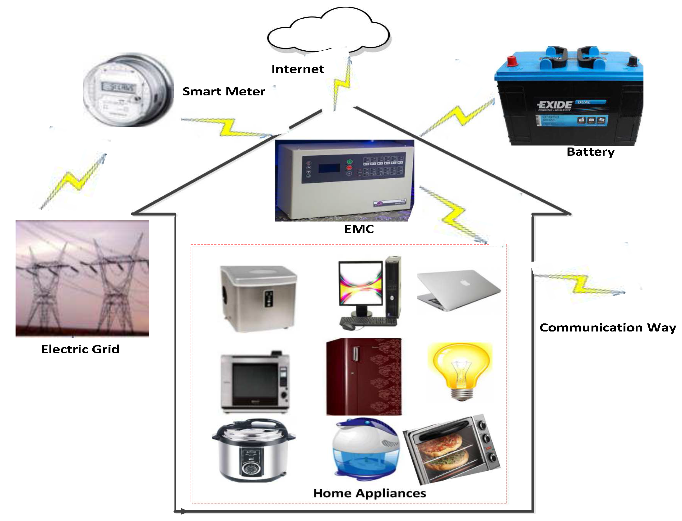
Efficient and reliable operations in the smart grid are empowered by DSM. DSM key functions are energy management and demand side control activities for electricity consumers. We assume a system model having a power system with a single utility and a smart building; comprised of 30 smart residential homes (apartments). The demand of the electricity consumers is met by the electric grid (utility) directly or ESS. Let $\mu$ denote the set of all electricity consumers in a building, and each consumer u ∈ $\mu$ has his/her own living pattern, i.e., Length of Operational Time (LOT) and power rating of appliances. In order to compute the hourly power consumption of each electricity consumer u, smart meters are installed at every residence to communicate the extracted information of consumers’ demand to the utility. It also communicates price information from the utility to the electricity consumer. We consider one day for our implementation, and the whole day is divided into 24 operational time slots, where each time slot consists of 1 h.

$$T=\{t_1,t_2,t_3,t_4,\dots \dots ,t_{24}\}$$

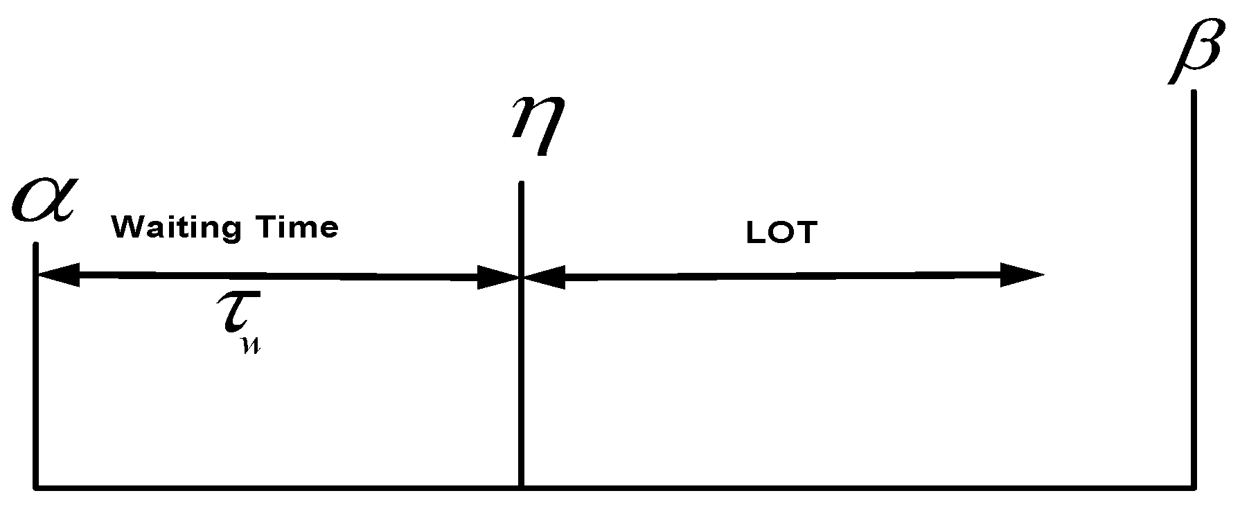
We categorized the home appliances based on the requirements of the electricity consumer; considering deferrable (a${}_d$), non-deferrable (a${}_{n}d$) and base load (a${}_b$) appliances where a${}_d$, a${}_{nd}$, a${}_b$ $ϵ$ A${}_n$ (i.e., A${}_n$ represents the set of all appliances). We assume that each appliance is capable of communicating with the Energy Management Controller (EMC), which is connected to the Internet. The EMC is an embedded computing platform that schedules the appliances depending on the availability of the time slot. Each appliance must complete its execution period between the earliest starting time and least finishing time. The execution pattern for each appliance is described in Figure 1, where $\alpha$ shows the earliest starting time, $\beta$ shows the least finishing time and $\eta$ nominates the time when the appliance starts its execution. The difference between $\alpha$ and $\eta$ shows the waiting time for each appliance. The earliest starting time and the least finishing time for each appliance are defined by the electricity consumer, explained in

Table 2. Parameters of appliances. LOT, Length of Operational Time.

Appliance Class	Appliance	Power Rating (kWh)	Earliest Starting Time (h)	Finishing Time (h)	LOT (h)
Base Load Appliances
	Cooker hub	3–4	6	10	1–3
	Cooker oven	4–5	15	20	1–3
	Microwave	1.7–2.5	6	10	1–3
	Laptop	0.1–0.2	18	24	2–4
	Desktop	0.3–0.5	18	24	3–5
	Vacuum cleaner	1.2–2	9	17	1–3
	Electrical car	3.5–5	18	8	3–5
Deferrable Appliances
	Dish washer	1.5–2	9	17	2–4
	Washing machine	1.5–2	7	12	2–3
	Spin dryer	2.5–3.5	13	18	1–3
Non-deferrable Appliances
	Interior lighting	0.84–1	16	24	6–8
	Refrigerator	0.3–0.5	1	24	22–24

. The proposed system model is illustrated in Figure 2.

The categorization of home appliances is done by the electricity consumers according to their requirements, and it can vary from time to time, i.e., in the summer season, the refrigerator is a non-deferrable appliance. However, the operation of the refrigerator is different in the winter season. Furthermore, we discuss in detail the categorization of home appliances and the mathematical formulation of the our proposed system in Section 3.1.

3.1. Assortment of Load

To evaluate the performance of our proposed system, we have considered two scenarios in our work. First, we implement our proposed system in a single smart home, and then, we investigate the performance of our proposed system on multiple smart homes. Each home has n number of smart appliances with different categories. These appliances are scheduled in a 24-h time horizon $t\in T$ according to electricity consumer preferences.

For the appliance scheduling problem, we consider twelve different basic appliances for all homes in a smart building; normally, every home consists of the mentioned appliances in [11].

3.1.1. Deferrable Appliances

In this work, the appliances that can be interrupted or shifted in any of the given time slots in a day depending on their necessity are called deferrable appliances. The dish washer, washing machine and spin dryer are included in this class. Let A${}_d$ denote the combination of deferrable appliances and $a_d\in A_d$ represent each appliance in the deferrable class. In Equation (1), ${\lambda }_d$ shows the power rating of every appliance in this class. The total electricity utilization ${\epsilon }_d$ of deferrable appliances in a day is shown by the following mathematical formula:

$${\epsilon }_d=\sum _{t=1}^T\left(\sum _{a_dϵA_d}{\lambda }_d\times {\alpha }_d\left(t\right)\right)$$

(1)

The total cost per hour that is paid by the consumer against all deferrable appliances can be calculated as:

$${\sigma }_{A_d}^t=\sum _{a_dϵA_d}({\lambda }_d\times \rho \left(t\right)\times {\alpha }_d\left(t\right))$$

(2)

The total cost of one day that is paid by the consumer to the utility against all deferrable appliances is given by the following equation:

$${\delta }_{A_d}^{Total}=\sum _{t=1}^T\left(\sum _{a_dϵA_d}({\lambda }_d\times \rho \left(t\right)\times {\alpha }_d\left(t\right))\right)$$

(3)

Here, ${\alpha }_d\left(t\right)$ represents the ON/OFF status of deferrable appliances in the form of one or zero.

$${\alpha }_d\left(t\right)=\left\{\begin{array}{c}1If{a}_{d}isON\hfill \\ 0If{a}_{d}isOFF\hfill \end{array}\right.$$

(4)

Similarly, the total electricity consumption and electricity cost for multiple smart homes against deferrable appliances in a day is calculated by Equations (5) and (6), respectively.

$${\vartheta }_d=\sum _{u=1}^{\mu }\left({\epsilon }_d\right)$$

(5)

$${\phi }_{A_d}^{Total}=\sum _{u=1}^{\mu }\left({\delta }_{A_d}^{Total}\right)$$

(6)

In Equation (5), ${\epsilon }_d$ represents the daily electricity consumption and ${\delta }_{a_d}^{Total}$ represents the daily cost for a single consumer in Equation (6).

3.1.2. Non-Deferrable Appliances

We consider an appliance non-deferrable, which cannot be shifted or interrupted while executing. These appliances need the right time slot for the completion of their execution. We assume the refrigerator and interior lighting as non-deferrable appliances. Let $a_{nd}\in A_{nd}$ represent each appliance in the class of non-deferrable appliances. The power rating of each appliance is ${\lambda }_{nd}$, and total energy utilization ${\epsilon }_{nd}$ per day is shown by the following mathematical formula:

$${\epsilon }_{nd}=\sum _{t=1}^T\left(\sum _{a_{nd}ϵA_{n}d}({\lambda }_{nd}\times {\alpha }_{nd}\left(t\right))\right)$$

(7)

Due to the un-interruptible and non-shiftable behavior of these appliances, consumers pay the maximum cost because for the demanded slot of these appliances, the utility has higher prices. The reason behind high prices is an increase in PAR. In order to maintain the balance between generation and consumption, the utility charges higher prices. The cost of each day for all appliances in the non-deferrable class can be computed using Equation (8).

$${\delta }_{A_{nd}}^{Total}=\sum _{t=1}^T\left(\sum _{a_{nd}ϵA_{n}d}({\lambda }_{nd}\times \rho \left(t\right)\times {\alpha }_{nd}\left(t\right))\right)$$

(8)

Similarly, the cost for non-deferrable appliances over an individual time slot can be computed according to Equation (9).

$${\sigma }_{A_{nd}}^t=\sum _{a_{nd}ϵA_{n}d}({\lambda }_{nd}\times \rho \left(t\right)\times {\alpha }_{nd}\left(t\right))$$

(9)

Here, ${\alpha }_{nd}\left(t\right)$ represents the ON/OFF status of non-deferrable appliances.

$${\alpha }_{nd}\left(t\right)=\left\{\begin{array}{c}1If{a}_{nd}isON\hfill \\ 0If{a}_{nd}isOFF\hfill \end{array}\right.$$

(10)

The total electricity consumption and electricity cost against non-deferrable appliances for $\mu$ number of users in an individual day is calculated by Equations (11) and (12), respectively.

$${\vartheta }_{nd}=\sum _{u=1}^{\mu }\left({\epsilon }_{nd}\right)$$

(11)

$${\phi }_{A_{nd}}^{Total}=\sum _{u=1}^{\mu }\left({\delta }_{A_{nd}}^{Total}\right)$$

(12)

3.1.3. Base Load Appliances

The third class of appliances is known as base load appliances, and these appliances consist of base load for every smart home. The operation time cannot be modified or interrupted for these types of appliances. However, the scheduler has to schedule base load appliances between the earliest starting and least ending time, which is defined by the consumers. Let $a_b\in A_b$ represent each appliance in this class. The power rating and energy consumption of these appliances can be demonstrated by ${\lambda }_b$ and ${\epsilon }_b$, respectively. Per day energy consumption is given in Equation (13).

$${\epsilon }_b=\sum _{t=1}^T\left(\sum _{a_bϵA_b}({\lambda }_b\times {\alpha }_b\left(t\right))\right)$$

(13)

Per hour electricity cost and total electricity cost against 24 h for a single smart home paid by consumers are calculated by Equations (14) and (15), respectively.

$${\sigma }_{A_b}^t=\sum _{a_bϵA_b}({\lambda }_b\times \rho \left(t\right)\times {\alpha }_b\left(t\right))$$

(14)

$${\delta }_{A_b}^{Total}=\sum _{t=1}^T\left(\sum _{a_bϵA_b}({\lambda }_b\times \rho \left(t\right)\times {\alpha }_b\left(t\right))\right)$$

(15)

The total electricity consumption and electricity cost that is paid against base load appliances for multiple homes in 24 h are explained in Equations (16) and (17), respectively.

$${\vartheta }_b=\sum _{u=1}^{\mu }\left({\epsilon }_b\right)$$

(16)

$${\phi }_{A_b}^{Total}=\sum _{u=1}^{\mu }\left({\delta }_{A_b}^{Total}\right)$$

(17)

Here, ${\alpha }_b\left(t\right)$ represents the ON/OFF status of base load appliances in the form of one or zero.

$${\alpha }_b\left(t\right)=\left\{\begin{array}{c}1IfbaseloadapplianceisON\hfill \\ 0IfbaseloadapplianceisOFF\hfill \end{array}\right.$$

(18)

3.2. Electricity Cost

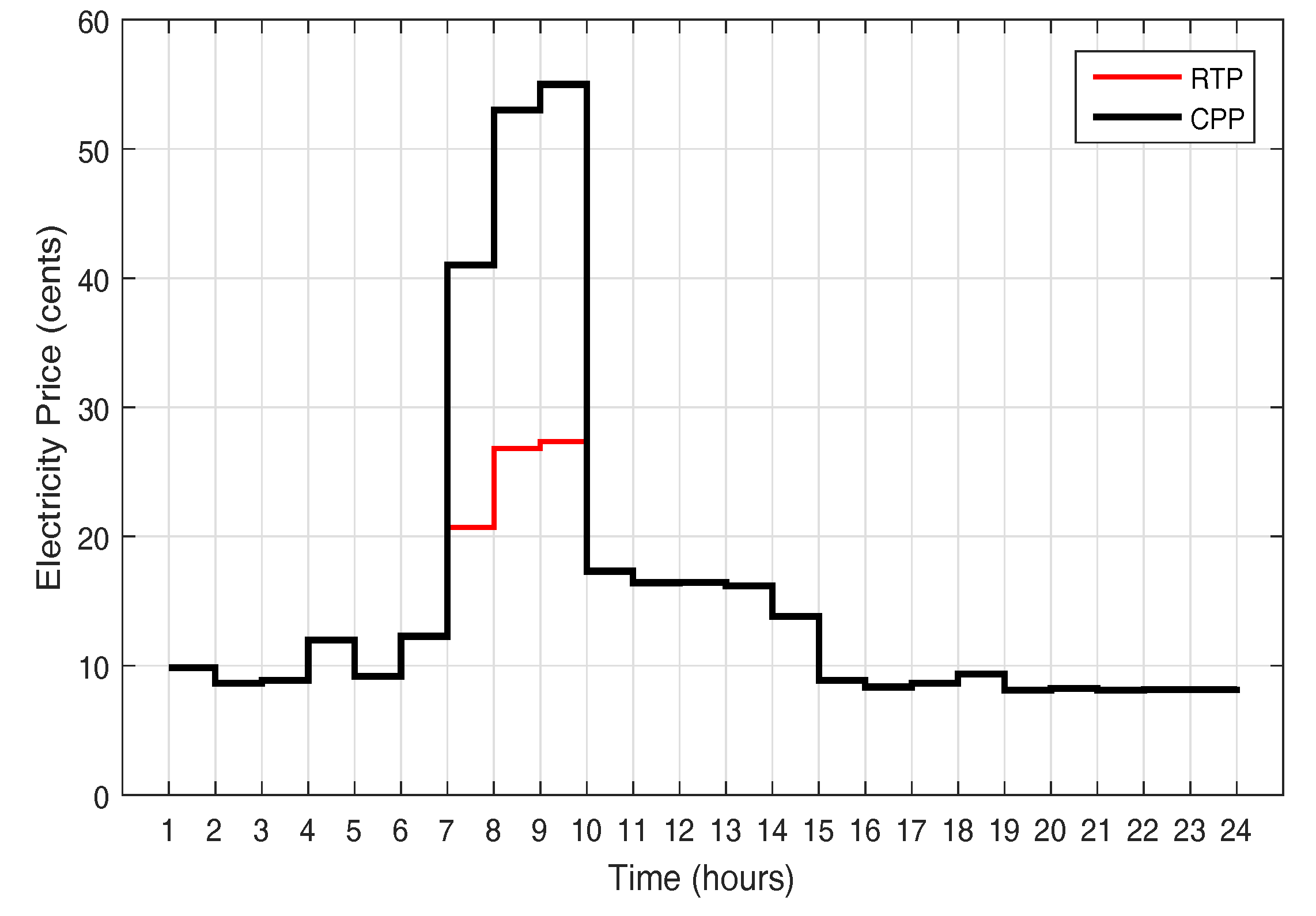
The cost is paid against the consumed electricity, which is calculated with respect to the per unit price of electricity. There are many schemes for defining per unit cost of electricity, provided by the utility to motivate consumers to manage their electricity load. Some of the pricing schemes are: ToU, CPP, IBR and RTP. In our work, RTP and CPP signals are used for electricity cost estimation, which are represented in Figure 3. The pricing scheme is represented by $\rho \left(t\right)$, for each time interval $tϵT$. The total electricity cost per hour for all classes is equal to the product of total load that is consumed in the particular time slot ‘t’ and the price signal $\rho$ in the same hour. The total electricity cost against the individual time slot for single and multiple smart homes is shown by Equations (19) and (20).

$${\sigma }^t=\sum _{a_d,a_{nd},a_b}({\lambda }_{a_d,a_{nd},a_b}\times \rho \left(t\right)\times \alpha \left(t\right))$$

(19)

$${\zeta }^t=\sum _{u=1}^{\mu }\left({\sigma }^t\right)$$

(20)

Similarly, the total cost per day against all types of appliances for single and multiple smart homes is computed by Equations (21) and (22), respectively.

$${\delta }^{Total}=\sum _{t=1}^{24}\left(\sum _{a_d,a_{nd},a_b}({\lambda }_{a_d,a_{nd},a_b}\times \rho \left(t\right)\times \alpha \left(t\right))\right)$$

(21)

$${\xi }^{Total}=\sum _{t=1}^T\left({\delta }^{Total}\right)$$

(22)

3.3. Electricity Storage System

We have assumed a small capacity ESS for the storage of electricity. Basically, ESS is integrated to exploit the efficiency of HEMS. ESS is a special type of deferrable electricity load, which can be shifted in any time slot in an adoptable way, i.e., charging and discharging of electricity. We have considered the ESS minimum storage level and maximum storage level to improve ESS efficiency, and the ESS charging must be less than or equal to the maximum charging level presented in Equation (23). We considered the minimum and maximum electricity storage levels of 10% and 90%, respectively, of the total capacity of ESS. ESS charges electricity only when the electricity price is low and the charging level of ESS is below the upper charging level limit explained in Equation (24). ESS discharges only when the electricity rate is high and ESS storage is more than the ESS minimum level explained in Equation (25).

$$E{S}_t^{ch}<=ES\left(max\right)$$

(23)

$$ES{S}_t^{ch}<ESS\left(upl\right)$$

(24)

$$E{S}_t^{dis}>=ES\left(min\right)$$

(25)

The stored electricity in ESS at time ‘t’ is explained by Equation (26) [24], the electricity charging and discharging taken into account. There are some electricity losses due to charging and discharging ESS; therefore, turn-around ESS efficiency is considered.

$$SE\left(t\right)=SE(t-1)+k·{\eta }^{ESS}·E{S}^{\left(ch\right)}\left(t\right)-k·E{S}^{dis}\left(t\right)/{\eta }^{ESS}$$

(26)

where $SE$ is the stored electricity in kWh at time ‘t’, k is the time slot (h), ${\eta }^{ESS}$ is the ESS efficiency, $E{S}^{\left(ch\right)}$ is charging to ESS at time ‘t’ and $E{S}^{dis}$ is the discharging from ESS at time ‘t’.

4. Proposed Schemes

In the smart grid, every smart home is connected with a smart meter, and the smart meter is further connected with an EMC. The smart meter and EMC permit the mutual two-way communication between electricity consumers and the utility. It inspires the consumer to perform load shifting from peak to off-peak hours for cost minimization. However, load shifting in off-peak hours may cause the generation of peaks in off-peak hours. This problem is considered as an optimization problem, and in the last few years, many techniques have been proposed to tackle this problem. However, no technique gave sufficient attention to minimizing the electricity cost and PAR with minimum user waiting time simultaneously. Therefore, the main targets of our work are electricity cost and PAR reduction with minimum user waiting time. For this optimization problem, three meta-heuristic techniques GA, CSA and CSOA are used. In this section, a brief introduction of GA, CSA and CSOA is presented, and then, the procedure of these heuristic techniques in our work is elaborated.

4.1. Genetic Algorithm

The GA is a well-known algorithm from the meta-heuristic algorithms, which is also called the global search algorithm. The GA shows effectiveness for solving high complexity and big problems because the convergence rate of GA is very high. Due to the high convergence rate, GA finds a very optimized solution for any computing problem. GA was explained in [26] and works on the basis of a genetic population like chromosomes. GA is actually used to solve the optimization problem in computing, and the solution is obtained in binary form (1,0); however, other encodings are also used for the solution. GA has three main steps for searching for the global solution. The first step is to initialize the population randomly; the evaluation of fitness is next step; and the last step of GA is the reproduction of the new population. Three main tasks, selection, crossover and mutation, are performed for the reproduction step.

In our scenario, GA starts searching from randomly-initialized (binary valued 1,0) chromosomes. The bit 1,0 shows the ON or OFF state of the home appliances, respectively. The total number of home appliances is represented by the length of chromosomes. A random population (or solution set) generated for a specific time interval shows the status of every appliance in the home. Every possible solution is evaluated according to the fitness function; which is PAR and cost minimization with minimum user waiting time. The new population (or solution set) is reproduced iteratively using crossover and mutation operators. In crossover, two parents are selected on the basis of fitness values, and new offspring are generated. The crossover probability of GA is represented by $p_c$ in Equation (27).

$$p_c=0.9$$

(27)

The mutation operator is used to bring changes in the new population by changing one or more bits. Mutation probability is very low in the natural genetic process, so best mutation probability is explained in Equation (28). The complete process restarted for searching for the global best solution, and the parameters of GA are explained in

Table 3. GA parameters.

Parameters	Values
Population size	200
Number of iterations	500
Crossover	0.90%
Mutation	0.10%
n	12

.

$$P_m=1-P_c$$

(28)

4.2. Cuckoo Search Optimization Algorithm

The Cuckoo Search Optimization Algorithm (CSOA) is a meta-heuristic nature-inspired algorithm, which is used to find the optimal solution of any computing problem. It is based on the reproduction behavior of some special types of cuckoo species and features of Lèvy flights of some birds as explained in [27]. Some cuckoos dump their eggs in other birds’ nests, called host nests. Host birds discover the eggs that are laid by other cuckoos for reproduction. The number of host nests is fixed, and the discovering probability of the host is $P\alpha$ = [0, 1]. CSOA provides the optimal solution through adopting the following three basic rules.

• Every cuckoo put only one egg at a moment in a nest, which is randomly selected.
• Only the nests containing a superior quality of eggs are selected for the next production.
• The quantity of host nests is constant, and the host birds discover the eggs that are laid by cuckoos.

In our work, the CSOA starts finding the local solution from randomly-laid eggs (in the form of 1,0) in the host nests. The pattern of eggs (1,0) represents the ON or OFF state of the home appliances respectively in a specific time interval. Every egg (possible solution) is evaluated according to our fitness function; which is cost minimization with minimum user waiting time and PAR. After searching for the local solution, the reproduction step is performed by cuckoos. The best quality eggs (local best solutions) are discovered by host cuckoos, and discovering probability rate is 0.250.

For the reproduction step, only the nests containing the best quality of eggs (best local solutions) are selected. To find the global best solution Lèvy flights are performed for generating new solutions $X^{(t+1)}$ for a Cuckoo${}_i$ [27].

$$X_i^{(t+1)}=X_i^{\left(t\right)}+\alpha \oplus Levy\left(\lambda \right),$$

(29)

By nature, animals or birds search for food randomly. A Lèvy flight is a random walk in which step lengths have a high probability distribution. It is performed for searching for the global best solution and generating randomness for the next generation. These steps continue till the global best solution is not found, and the parameters of CSOA are explained in

Table 4. Cuckoo Search Optimization Algorithm (CSOA) parameters.

Parameters	Values
Number of host nests	50
Number of iterations	2000
Discovery rate	0.250
n	12

.

4.3. Crow Search Algorithm

The CSA is meta-heuristic algorithm based on the very intelligent behavior of crows, proposed in [28]. The crows have the largest brain according to their body size. Crows save/hide their food in different places for future use and can remember the faces of other birds and food hiding points for some months. Moreover, crows can communicate with each other and remember the faces of each other. Crows can try to obtain the information about places where the other birds/crows save their food, then steal the food when the owners of the food leave the food hiding place. In reality, crows can determine the risk-free places to secure their collected food from being stolen using their own experience of having been a thief to predict the behavior of a thief. The parameters of CSA are shown in

Table 5. Crow Search Algorithm (CSA) parameters.

Parameters	Values
Flock size	100
Number of iterations	100
Fight length	2
Awareness probability	0.10
n	12

.

The CSA follows the four basic principles mentioned below:

• Crows live in the form of a group.
• Crows remember the the hiding places.
• Crows follow each other to steal food.
• Crows secure their collected food from being stolen by a probability.

In our work, CSA starts searching for the positions (local solutions) from random hiding places on the basis of the large memory of crows, where the other birds’ food is hidden. In this study, we have considered a 0.10 awareness probability of crows. Every solution shows the appliance in the form of zero or one (OFF or ON). At any position, when a crow finds the food (best solution according to our fitness function), this is considered the best position, and the appliance is ON, otherwise OFF. After collecting all food hiding positions (local solutions), it finds out the global best solution by comparing all local solutions.

5. Feasible Region

A region that is covered by a set of some points containing all possible solutions according to our fitness function is called the feasible region. In this optimization problem, our target is to minimize the electricity cost and reduce PAR. Hence, electricity cost is based on these two main factors: electricity consumption and electricity price, which is offered by the utility in a specific time horizon; and we have no authority over electricity price. However, we have authority on load only via shifting load from high price to low price hours to achieve our target. For electricity cost calculation, we have the following four situations using pricing signals:

• Minimum load, minimum price.
• Minimum load, maximum price.
• Maximum load, maximum price.
• Maximum load, minimum price.

The waiting time of the user also affects the electricity cost. Therefore, we calculate the feasible region of electricity cost with user waiting time. When user waiting time is maximal, the electricity cost is low, and when waiting time is minimal, electricity cost is high. The feasible region of electricity cost and user waiting time lies in the following conditions:

• Minimum waiting time, minimum cost.
• Minimum waiting time, maximum cost.
• Maximum waiting time, minimum cost.
• Maximum waiting time, maximum cost.

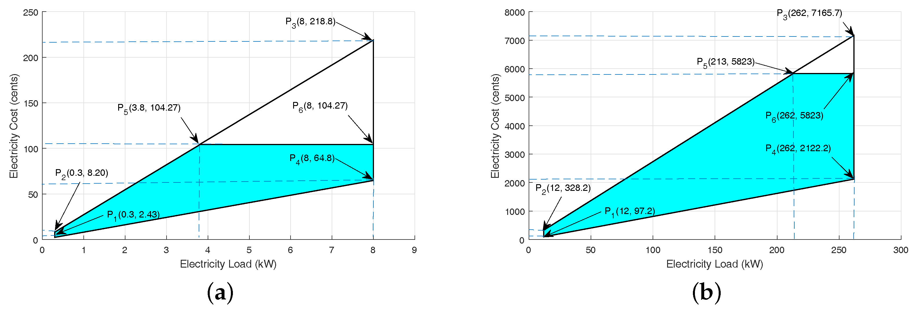
5.1. Feasible Region for Electricity Cost and Electricity Consumption Using RTP Signals

The feasible region of the electricity cost for multiple smart homes using RTP signals is represented in Figure 4b. An area that is covered by these points, p${}_1$(12, 97.2), p${}_2$(12, 328.2), p${}_3$(262, 7165.7), p${}_4$(262, 2122.2), p${}_5$(213, 5823) and p${}_6$(262, 5823), demonstrates the feasible region of the electricity consumption cost for multiple homes; where p${}_1$(12, 97.2) shows the minimum electricity cost against the minimum electricity consumption and minimum electricity rate for any time interval ‘t’; p${}_2$(12, 328.2) represents the maximum cost against the minimum electricity consumption and maximum electricity price for any time interval ‘t’; moreover, p${}_1$(12, 97.2) and p${}_2$(12, 328.2) represent the electricity consumption cost when the maximum appliances are in the off status in the minimum and maximum electricity rates, respectively.

However, p${}_3$(262, 7165.7) and p${}_4$(262, 2122.2) represent the maximum and minimum cost against the same electricity consumption with maximum and minimum electricity rates accordingly. This means the electricity cost through load scheduling must not exceed the unscheduled cost for any time interval ‘t’, which is 5823 cents. After implementing the threshold of 5823 cents with respect to electricity consumption cost, the feasible region of electricity consumption cost is shown by the pentagon of p${}_1$(12, 97.2), p${}_2$(12, 328.2), p${}_4$(262, 2122.2), p${}_5$(213, 5823) and p${}_6$(262, 5823); where the p${}_4$(262, 2122.2) and p${}_6$(262, 5823) show the minimum and maximum electricity cost with the same electricity consumption, and for unscheduled electricity consumption, the maximum load limit is 262 kW. Therefore, scheduled scenario electricity consumption in any time interval ‘t’ must not exceed the load limit, which is defined in p${}_4$(262, 2122.2).

The feasible region of electricity cost and consumption for a single smart home is represented in Figure 4a. In Figure 4a, an area is shown that is the combination of these points: p${}_1$(0.3, 2.43), p${}_2$(0.3, 8.20), p${}_3$(8, 218.8), p${}_4$(8, 64.8), p${}_5$(5.9, 104.27) and p${}_6$(8, 104.27) is the feasible region of electricity cost and electricity consumption for a single smart home. Here, p${}_1$(0.3, 2.43) and p${}_2$(0.3, 8.20) represent the minimum and maximum electricity cost with minimum load 0.3 kW, and p${}_3$(8, 218.8) and p${}_4$(8, 64.8) represent the minimum and maximum electricity cost with maximum electricity consumption. In the scheduled case, electricity cost must not increase the limit of the maximum electricity cost for any time period. The maximum electricity cost limit is 104.27, which is represented in point p${}_6$(8, 104.27) with maximum electricity consumption of 8 kW.

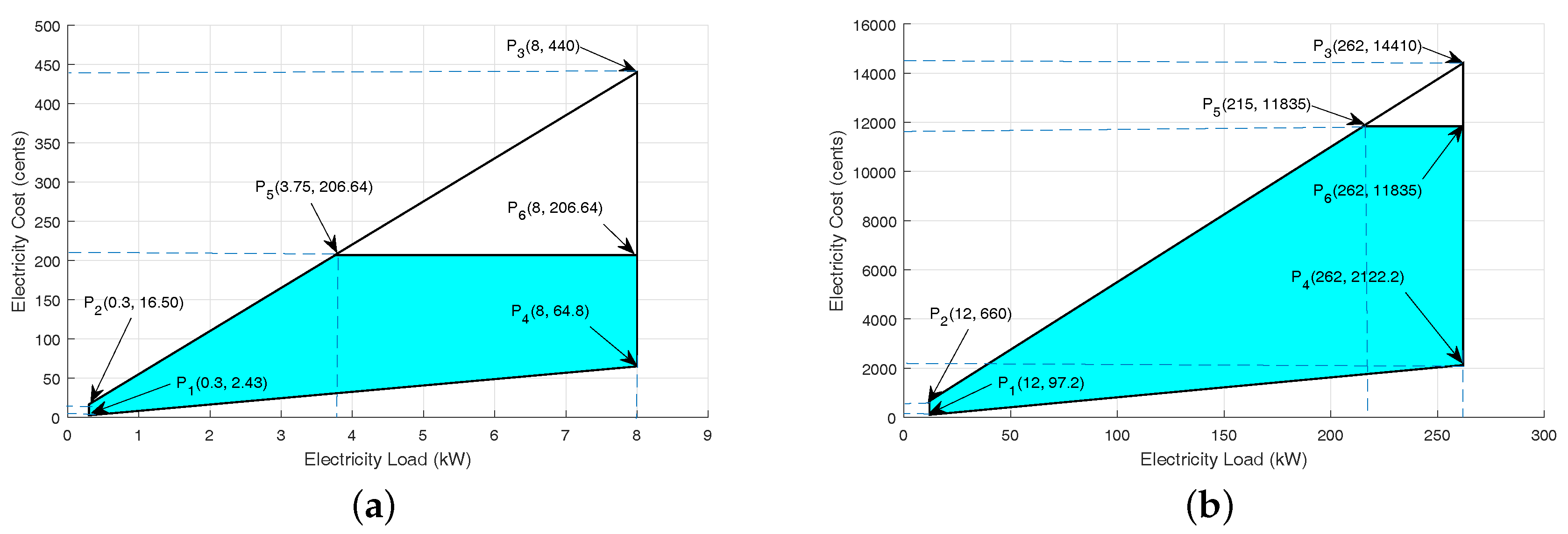
5.2. Feasible Region for Electricity Cost and Electricity Consumption Using CPP Signals

Figure 5a,b demonstrates the feasible region for electricity cost and electricity consumption against single and multiple smart homes using CPP signals. In Figure 5a, an area that is covered by these points: p${}_1$(0.3, 2.43), p${}_2$(0.3, 16.50), p${}_3$(8, 440), p${}_4$(8, 64.8), p${}_5$(3.75, 206.64) and p${}_6$(8, 206.64), shows the feasible region of the electricity cost and electricity consumption for a single smart home; where the points p${}_1$(0.3, 2.43) and p${}_4$(8, 440) represent the minimum and maximum electricity cost with minimum and maximum electricity consumption, respectively. When we implement the threshold of 206.64 cents on electricity cost, the feasible region of electricity cost is shown by the pentagon of the following points: p${}_1$(0.3, 2.43), p${}_2$(0.3, 16.50), p${}_4$(8, 64.8), p${}_5$(3.75, 206.64) and p${}_6$(8, 206.64). Points p${}_5$(3.75, 206.64) and p${}_6$(8, 206.64) clearly show that electricity cost is the same with different electricity consumptions. Therefore, in the scheduled case, electricity cost for any time interval t must not exceed the threshold, which is 206.64 cents.

Figure 5b represents the feasible region for cost and electricity consumption against multiple smart homes using CPP signals. The combination of these points p${}_1$(12, 97.2), p${}_2$(12, 660), p${}_3$(262, 14,410), p${}_4$(262, 2122.2), p${}_5$(215, 11,835) and p${}_6$(262, 11,835) shows the feasible region in Figure 5b. The points p${}_1$(12, 97.2) and p${}_2$(12, 660) represent the minimum and maximum electricity cost with the same load, which is 12 kW. The points p${}_3$(262, 14,410) and p${}_4$(262, 2122.2) show the maximum electricity load 262 kW with minimum and maximum electricity cost. However, after implementing the cost limit, which is 11,835 cents with maximum load 262 kW, the electricity cost for any time slot ‘t’ must not exceed the defined limit.

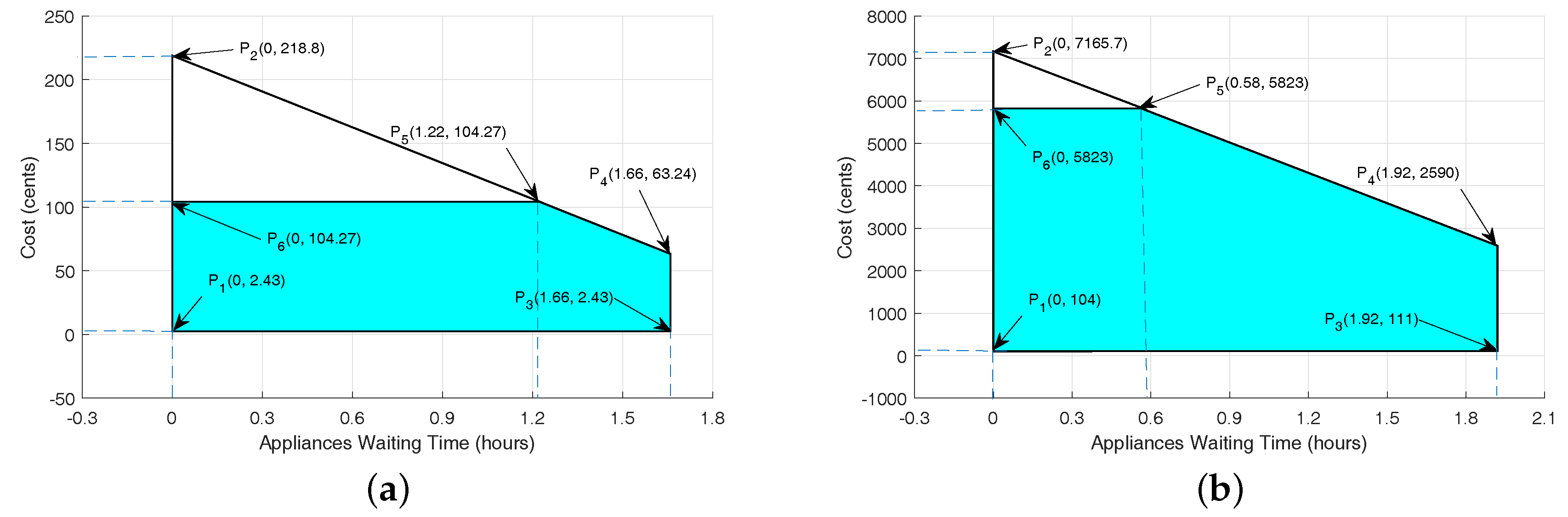
5.3. Feasible Region for Electricity Cost and User Waiting Time Using RTP Signals

The feasible region of electricity cost and user waiting time for multiple homes is represented in Figure 6b. A region that is covered by these points: p${}_1$(0, 104), p${}_2$(0, 6654), p${}_3$(1.92, 111), p${}_4$(1.92, 2590), p${}_5$(0.63, 5823) and p${}_6$(0, 5823), shows the feasible region of electricity cost with user waiting time for multiple smart homes; where the points p${}_1$(0, 104) and p${}_2$(0, 6654) demonstrate the minimum and maximum electricity cost with no waiting time. However, p${}_3$(1.92, 111) and p${}_4$(1.92, 2590) represent the minimum and maximum cost with the same waiting time; the waiting time is 1.92 (h). The point p${}_2$(0, 6654) represents maximum user discomfort because the user pays the maximum cost of 6654 cents against zero waiting time. Therefore, p${}_2$(0, 6654) was excluded from feasible region by implementing the maximum electricity cost limit, which is 5823 cents in any time slot ‘t’. However, p${}_5$(0.58, 5823) and p${}_6$(0, 5823) show the same electricity cost at different waiting times. This means deferrable appliances can minimize reasonable electricity cost by reducing their electricity demand during peak hours without increasing user waiting time.

Figure 6a shows the feasible region of electricity cost with user waiting time for a single smart home. A feasible region of electricity cost and user waiting time is generated with concatenation of these six points: p${}_1$(0, 2.43), p${}_2$(0, 218.8), p${}_3$(1.66, 2.43), p${}_4$(1.66, 63.24), p${}_5$(1.22, 104.27) and p${}_6$(0, 104.27). Minimum waiting time with minimum and maximum electricity cost is represented by the points p${}_1$(0, 2.43) and p${}_2$(0, 80), respectively. Points p${}_3$(1.66, 2.43) and p${}_4$(1.66, 63.24) demonstrate the maximum user waiting time with minimum and maximum electricity cost, respectively. The electricity consumer pays maximum electricity cost of 218.8.27 cents without waiting time on point p${}_2$(0, 218.8). After implementing the maximum electricity cost limit, which is 104.27 cents, p${}_2$(0, 218.8) is negated from the feasible region, which is shown in Figure 6a. Points p${}_5$(1.2, 104.27) and p${}_6$(0, 104.27) represent the same electricity cost with different user waiting times. Therefore, the electricity consumer can minimize the electricity cost via maximum consumption in off-peak hours.

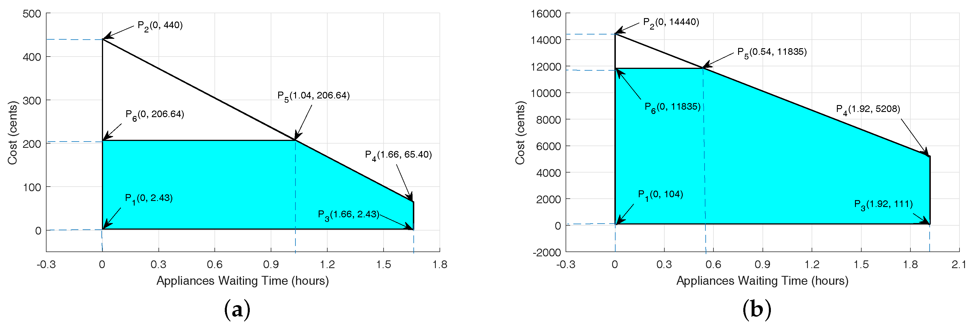
5.4. Feasible Region for Electricity Cost and User Waiting Time Using CPP Signals

The feasible region of electricity cost with user waiting time for single and multiple smart homes using CPP signals is demonstrated in Figure 7a,b, respectively. In Figure 7a, an area covered by these points: p${}_1$(0, 2.43), p${}_2$(0, 440), p${}_3$(1.66, 2.43), p${}_4$(1.66, 65.40), p${}_5$(1.04, 206.64) and p${}_6$(0, 206.64), shows the feasible region for a single smart home using CPP signals. In this region, points p${}_1$(0, 2.43) and p${}_2$(0, 440) represent the minimum cost of 2.43 cents and maximum cost of 440 cents with no waiting time. However, points p${}_3$(1.66, 2.43) and p${}_4$(1.66, 65.40) show the minimum and maximum cost with maximum waiting time of 1.66 h. After implementing the maximum cost limit of 206.64 cents, electricity cost must be less than the defined limit. When we excluded the point p${}_2$(0, 440) due to the higher cost compared to points p${}_5$(1.04, 206.64) and p${}_6$(0, 206.64), the electricity cost limit is 206.64 cents with the waiting time of 0 and 1.04 h. This clearly demonstrates that we minimize the electricity cost with bearable waiting time.

In Figure 7b, a region overspread by the following points, p${}_1$(0, 104), p${}_2$(0, 14,440), p${}_3$(1.92, 111), p${}_4$(1.92, 5208), p${}_5$(0.54, 11,835) and p${}_6$(0, 11,835), shows the feasible region against electricity cost with user waiting time for multiple smart homes using CPP signals. However, we negate the point p${}_2$(0, 14,440), due to the high cost with zero waiting time, by implementing a threshold on the electricity cost. The threshold is 11,835 cents, which is shown on points p${}_5$(0.54, 11,835) and p${}_6$(0, 11,835) with 0 and 0.54 h waiting time. After excluding the point p${}_2$(0, 14,440), the feasible region of electricity cost and user waiting is time shown by the following five points: p${}_1$(0, 104), p${}_3$(1.92, 111), p${}_4$(1.92, 5208), p${}_5$(0.54, 11,835) and p${}_6$(0, 11,835). This clearly shows that the users can reduce their electricity cost with affordable waiting time.

6. Computational Results, Presentation and Discussion

To show the legitimacy and productiveness of our proposed work, we have considered two scenarios for simulations in order to show an optimal scheduling for both single and multiple smart homes: (i) HEMS without ESS and (ii) HEMS with ESS. The randomization is one of the key factors in heuristic techniques; therefore, we have taken the results of the average of 10 runs. The effectiveness of our proposed work is evaluated in terms of electricity cost and PAR minimization with minimum user waiting time. Three meta-heuristic algorithms are implemented to analyze the performance of our proposed scheme. We design a model for a smart building, comprised of 30 smart homes (apartments), where each smart home has 12 smart appliances with different living patterns (i.e., length of operation and power rating).

Additionally, these 12 appliances are divided into three classes explained in Section 3. Different frameworks of all appliances may be obtained from the consumers (i.e., LOT, earliest starting time and least ending time). All the appliances with their parametric values that are used in our simulations are shown in Table 2. Non-deferrable appliances do not play any significant role in managing load because these are not scheduled and must perform their operation in time. Deferrable and base load appliances may contribute a huge part toward reducing PAR and minimizing electricity cost via shifting from high price hours to low price hours.

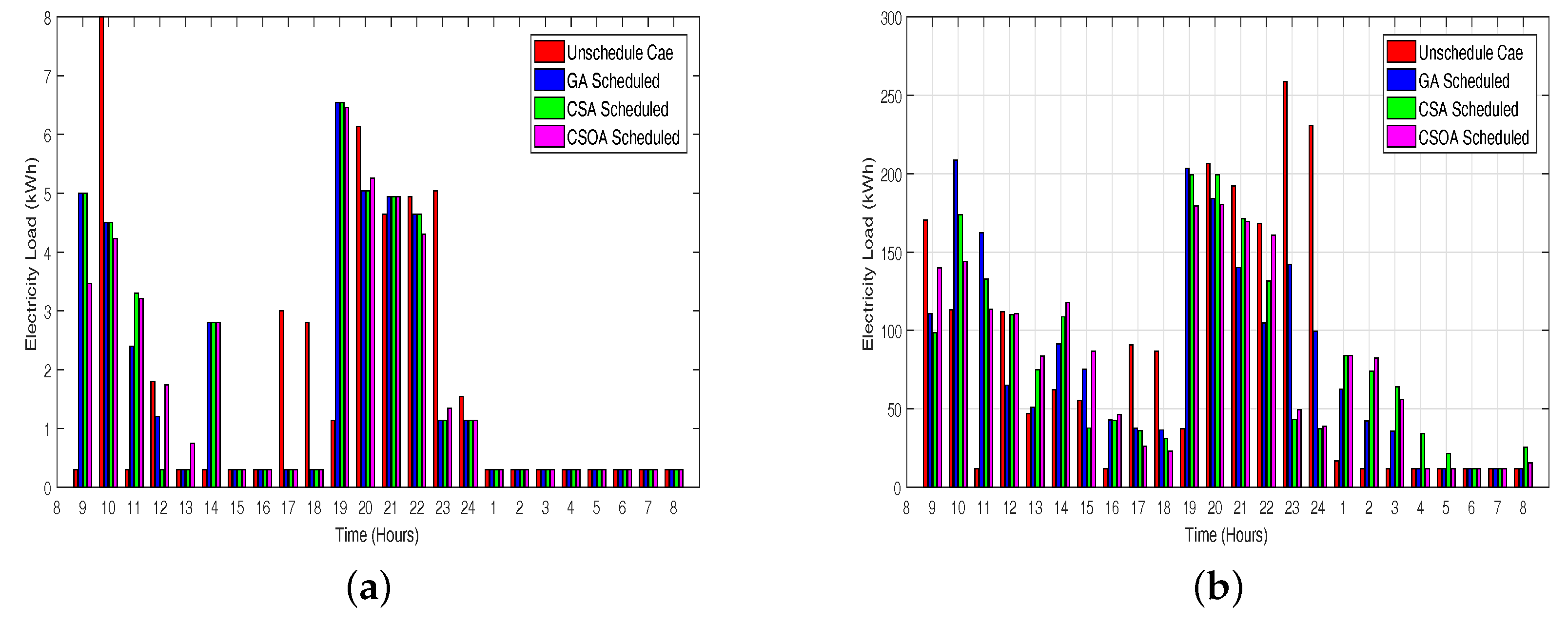
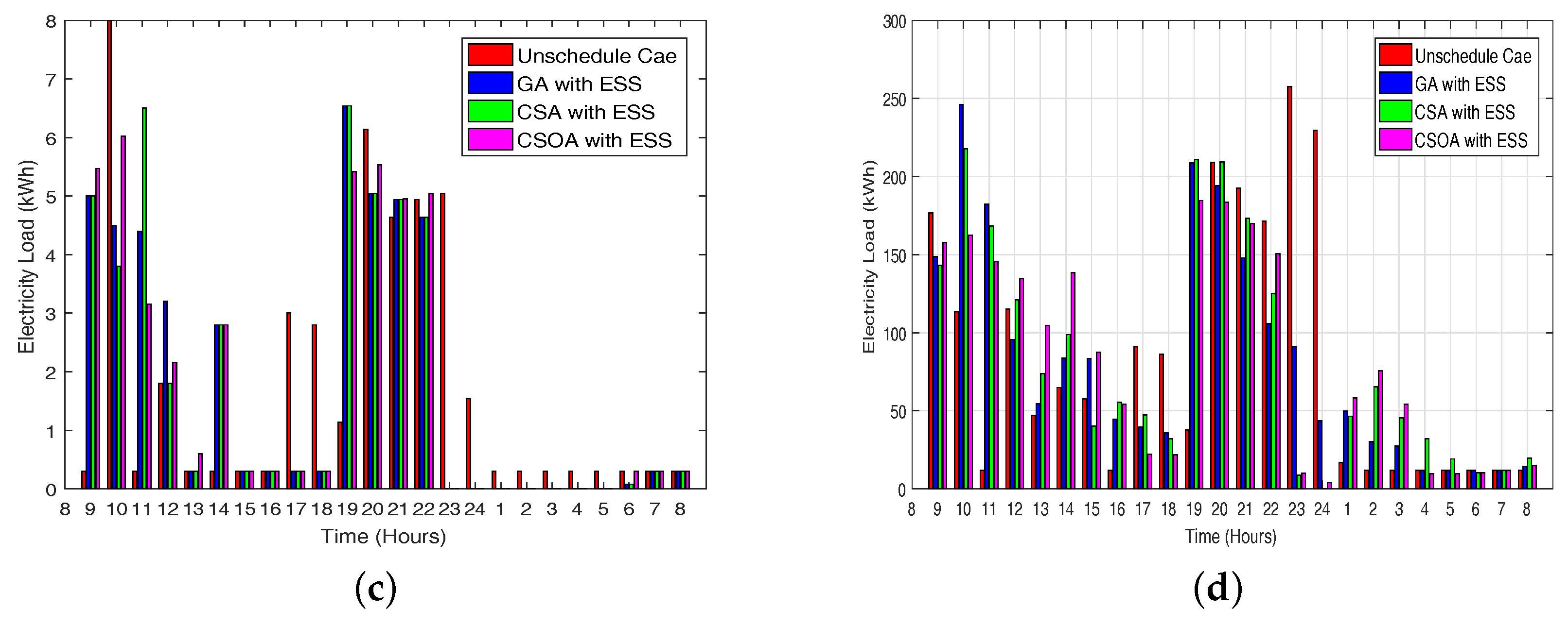
The time horizon is comprises of 24 time slots in a day, starting from 8 a.m.–8 a.m. the next day. Total electricity consumption per hour with ESS and without ESS for a single smart home and smart building is shown in Figure 8a–d, respectively. This clearly demonstrates that before implementing our proposed scheme, electricity consumption is high during peak hours. However, through our proposed scheme, electricity consumption is lower than the unscheduled consumption during peak hours. The electricity consumption is more minimized in high price hours using ESS as compared to HEMS without using ESS, explained in Figure 8c,d. This shows that our proposed schemes perform better for load transferring without interrupting the overall electricity consumption.

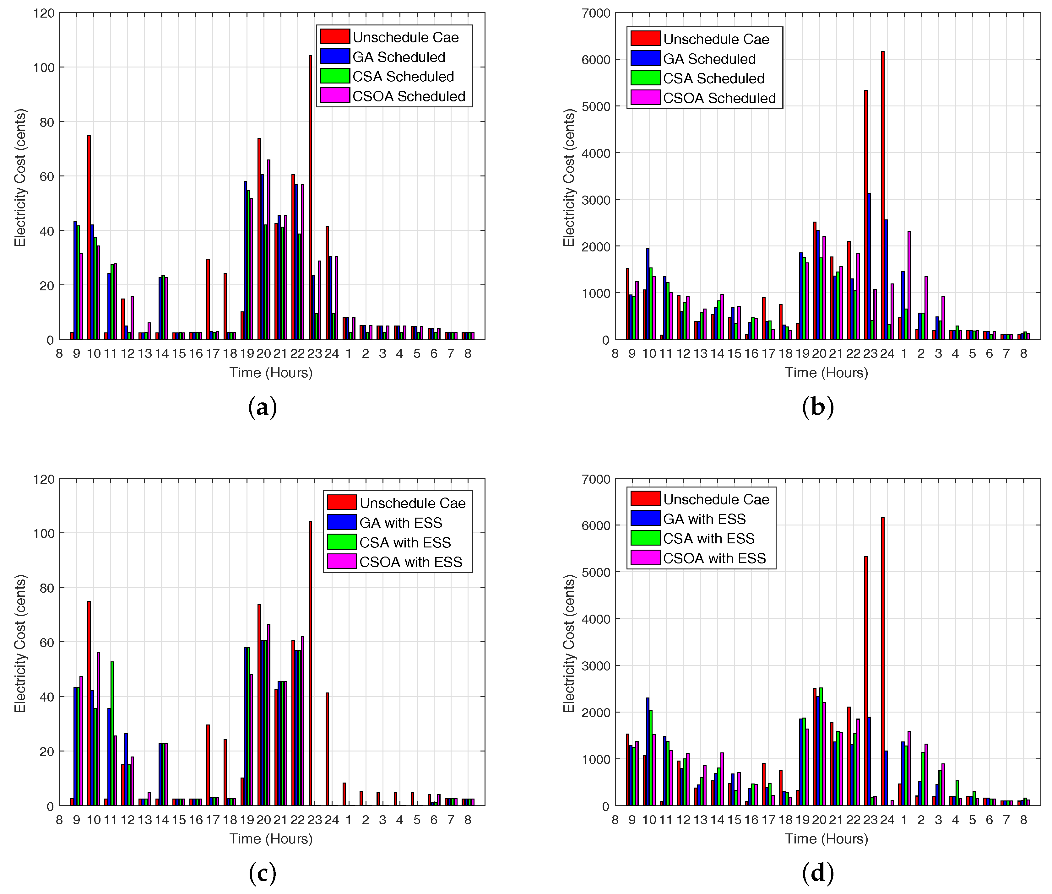
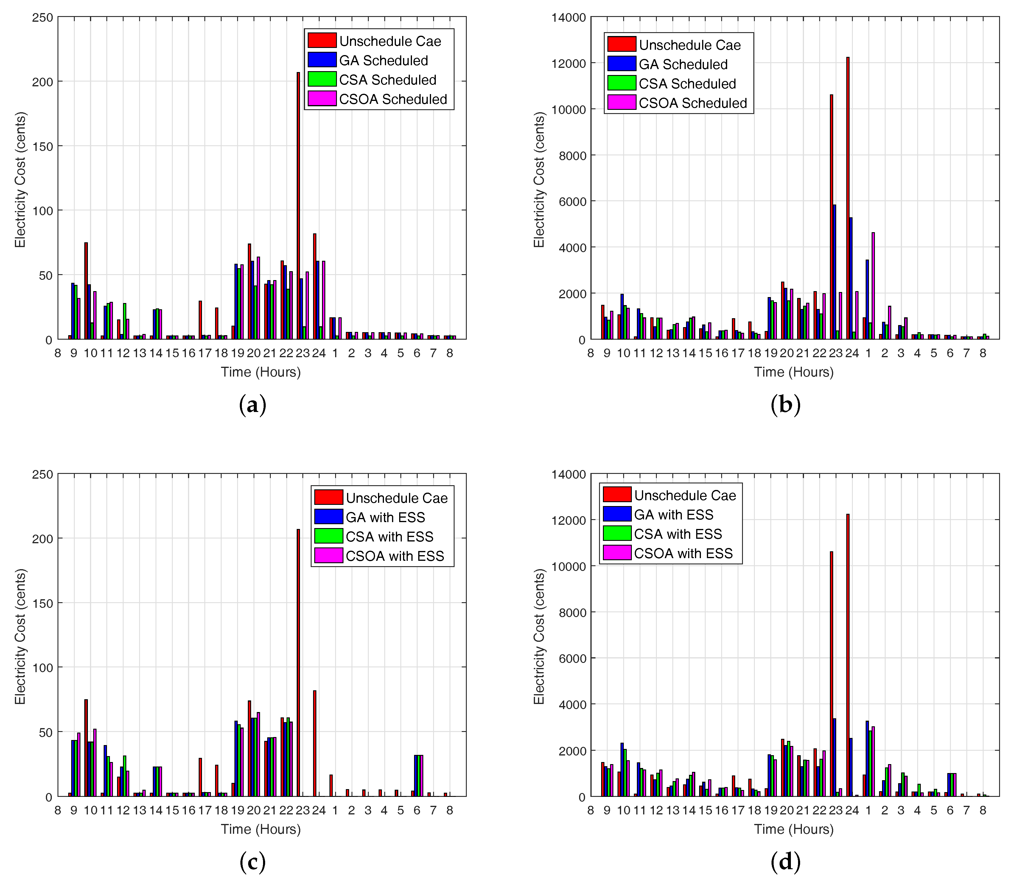
Figure 8a–d represents that CSOA shows supremacy in terms of load balancing as compared to GA, CSA and the unscheduled case. Furthermore, no peak is created during off peak hours. The per hour electricity cost with RTP signals HEMS with ESS and without ESS for unscheduled load and scheduled load through CSOA, GA and CSA for a single smart home and multiple smart homes in a building is shown in Figure 9a–d, respectively. We minimize per hour electricity cost, and as a result, total electricity cost per day is reduced, which is represented for single and multiple smart homes using RTP signals in Figure 9a–d, respectively.

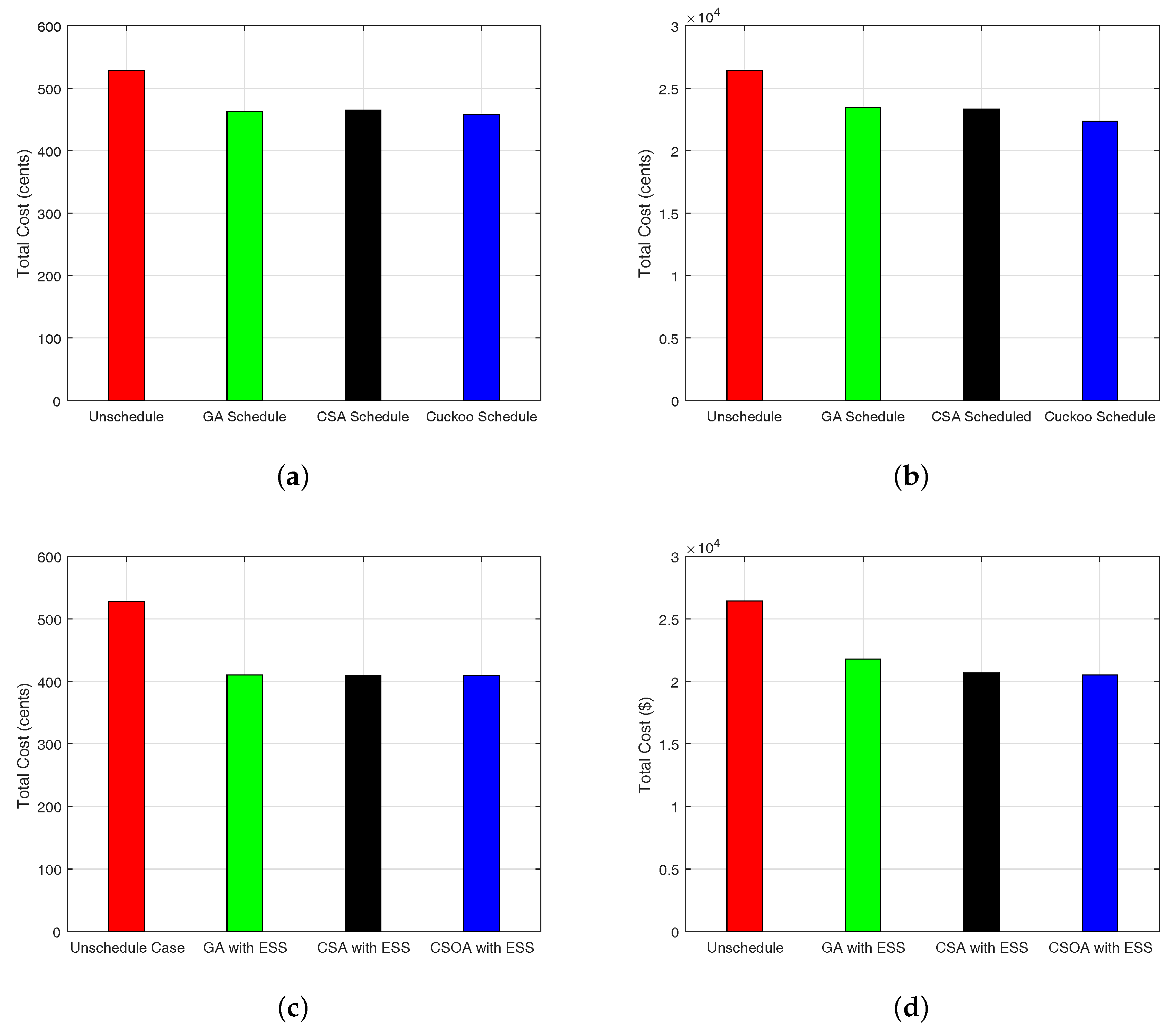
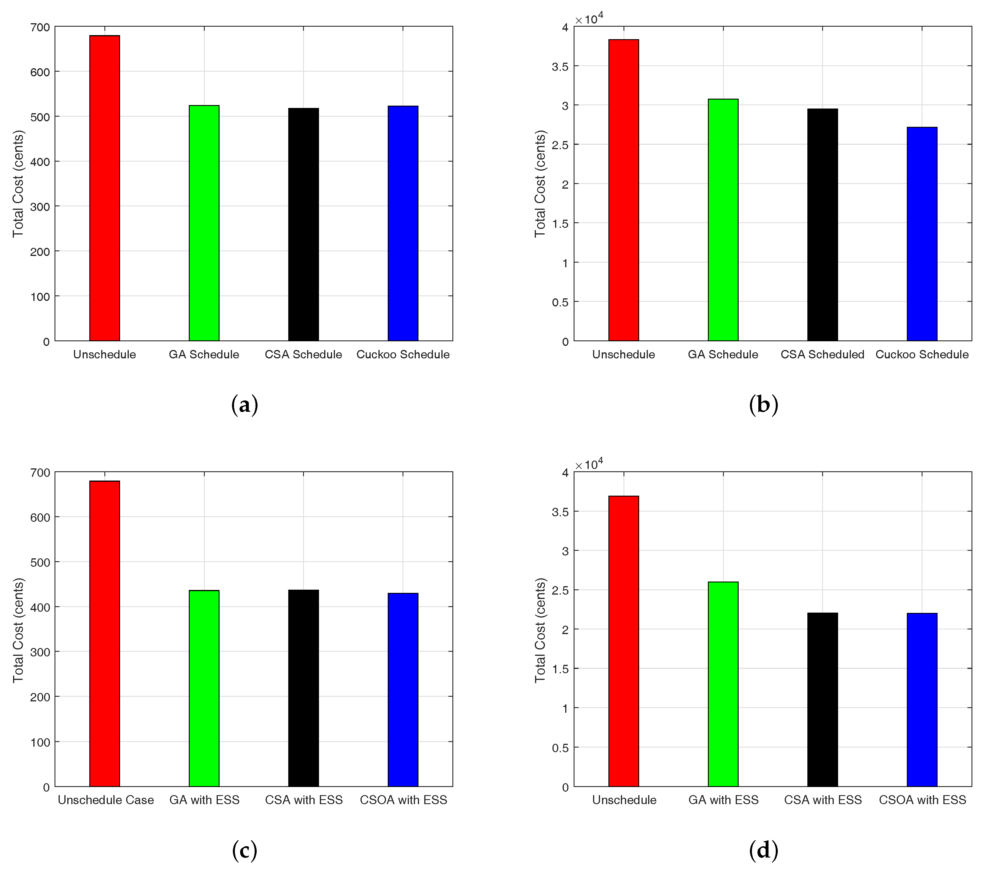
Figure 10a–d shows the total electricity cost using RTP signals. Using RTP signals without ESS GA, CSA and CSOA reduces the electricity cost by 12.57%, 14.44% and 12.33% for a single smart home and minimizes the cost by 11.95%, 13.12% and 14.97% for multiple (30) smart homes. Furthermore, the electricity cost reduction via RTP signals with ESS using GA, CSA and CSOA is 22.34%, 22.30% and 23.30%, respectively, for a single smart home. The cost reduction for multiple smart homes via the RTP signal with ESS using GA, CSA and CSOA is 16.61%, 21.11% and 23.02%, respectively. The result demonstrates that the electricity cost is low when ESS is used as compared to without ESS.

The electricity cost against individual time slots using CPP signals with ESS and without ESS is represented in Figure 11a–d for single and multiple smart homes, respectively. The results show that our proposed system with ESS performs superior compared to HEMS without ESS. The total cost in a day using CPP is represented in Figure 12a–d for single and multiple smart homes. The results show that electricity cost is low using CSOA, GA and CSA as compared to unscheduled electricity consumption. Furthermore, the total electricity cost of HEMS with ESS is low when we compare with HEMS without ESS.

Electricity cost reduced without ESS by GA, CSA and CSOA using CPP signals is 22.94%, 25.44% and 22.05% for a single smart home, respectively, and with ESS electricity, the cost reduction is 35.29%, 36.76% and 38.97% using GA, CSA and CSOA accordingly. Electricity cost reduction in multiple smart homes using GA, CSA and CSOA under CPP signals is 22.07%, 25.09 and 29.38%, respectively. The electricity cost reduction for multiple homes with CPP signals is 31.34%, 40.74% and 41.78% using GA, CSA and CSOA. A summary of the results is shown in

Table 6. Summary of the results for a single smart home.

Technique	Electricity Cost		Electricity Cost Saving
Pricing Scheme	RTP	CPP	RTP	CPP
Unscheduled	528	679.17	0%	0%
GA without ESS	465	524.03	11.93%	22.83%
GA with ESS	410	440	22.34%	35.29%
CSA without ESS	464	522	11.98%	23.12%
CSA with ESS	412	430	22.30%	36.76%
CSOA without ESS	459	520	13.06%	23.41%
CSOA with ESS	405	415	23.30%	38.97%

and

Table 7. Summary of the results for thirty smart homes.

Technique	Electricity Cost		Electricity Cost Saving
Pricing Scheme	RTP	CPP	RTP	CPP
Unscheduled	26546	38306	0%	0%
GA without ESS	23467	30752	11.59%	19.72%
GA with ESS	22135	26300	16.61%	31.34%
CSA without ESS	23450	29752	11.66%	22.93%
CSA with ESS	20940	22700	21.11%	40.74%
CSOA without ESS	22356	27150	15.78%	29.12%
CSOA with ESS	20435	22300	23.02%	41.78%

for single and multiple homes, respectively. The compared results show the supremacy of the proposed model using CSOA over other counterparts.

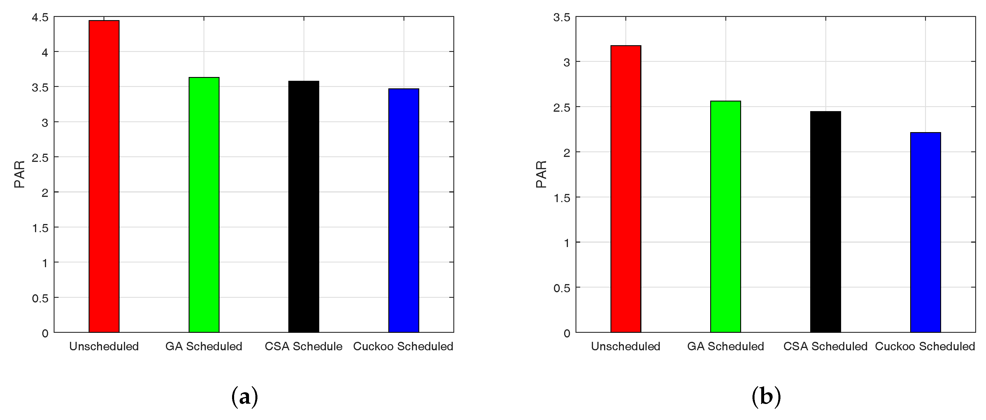
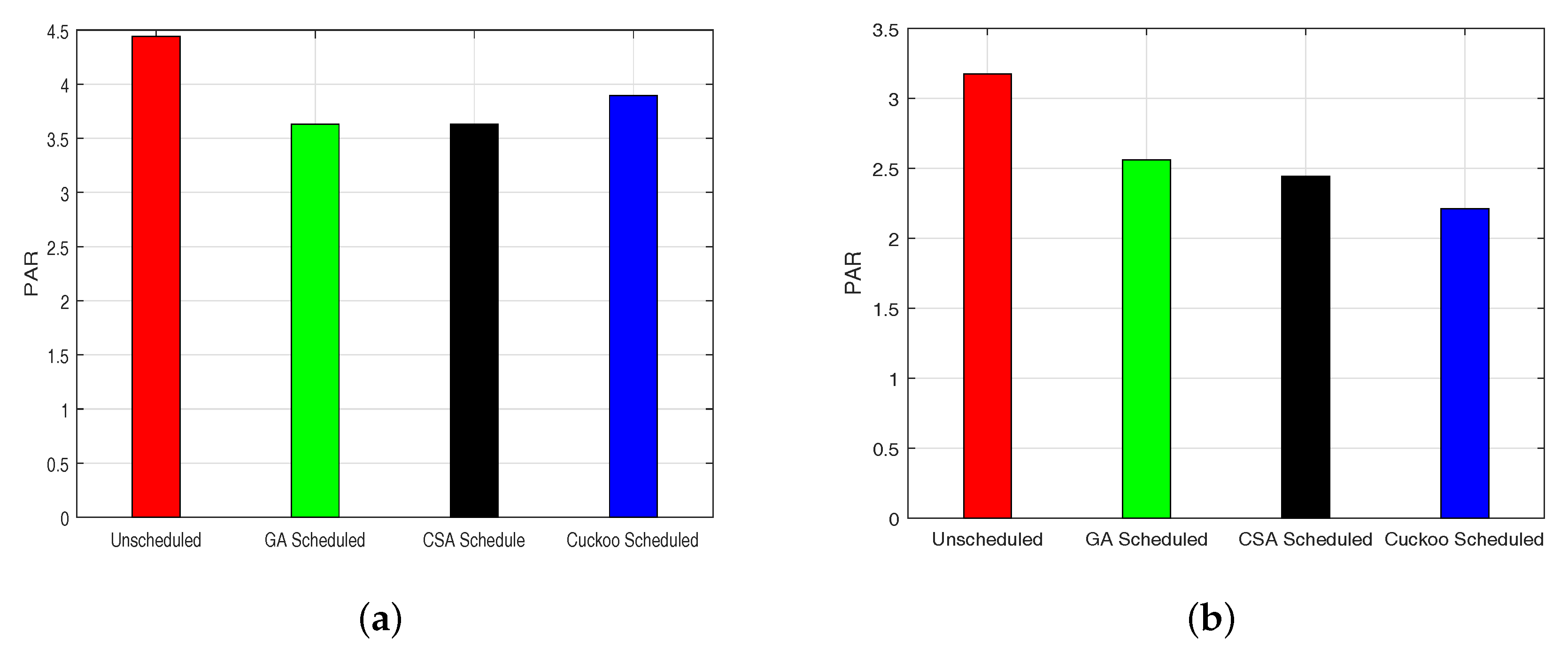
The minimization in PAR maximizes the stability of the electric grid and ensures the stable and reliable grid operations. PAR results using RTP signals are shown in Figure 13a,b, which distinctly shows that our proposed model minimizes the PAR as compared to unscheduled PAR. Furthermore, PAR reduction using GA, CSA and CSOA is 15.90%, 16.10% and 22.72%, respectively, for single smart homes, while there is a 21.72%, 22.34% and 30.35% PAR reduction for multiple smart homes using GA, CSA and CSOA, respectively. Figure 14a,b demonstrates the PAR results using CPP signals, which show the supremacy of our proposed scheme. The above discussions show that CSOA shifts load in a more efficient manner as compared to other counterparts.

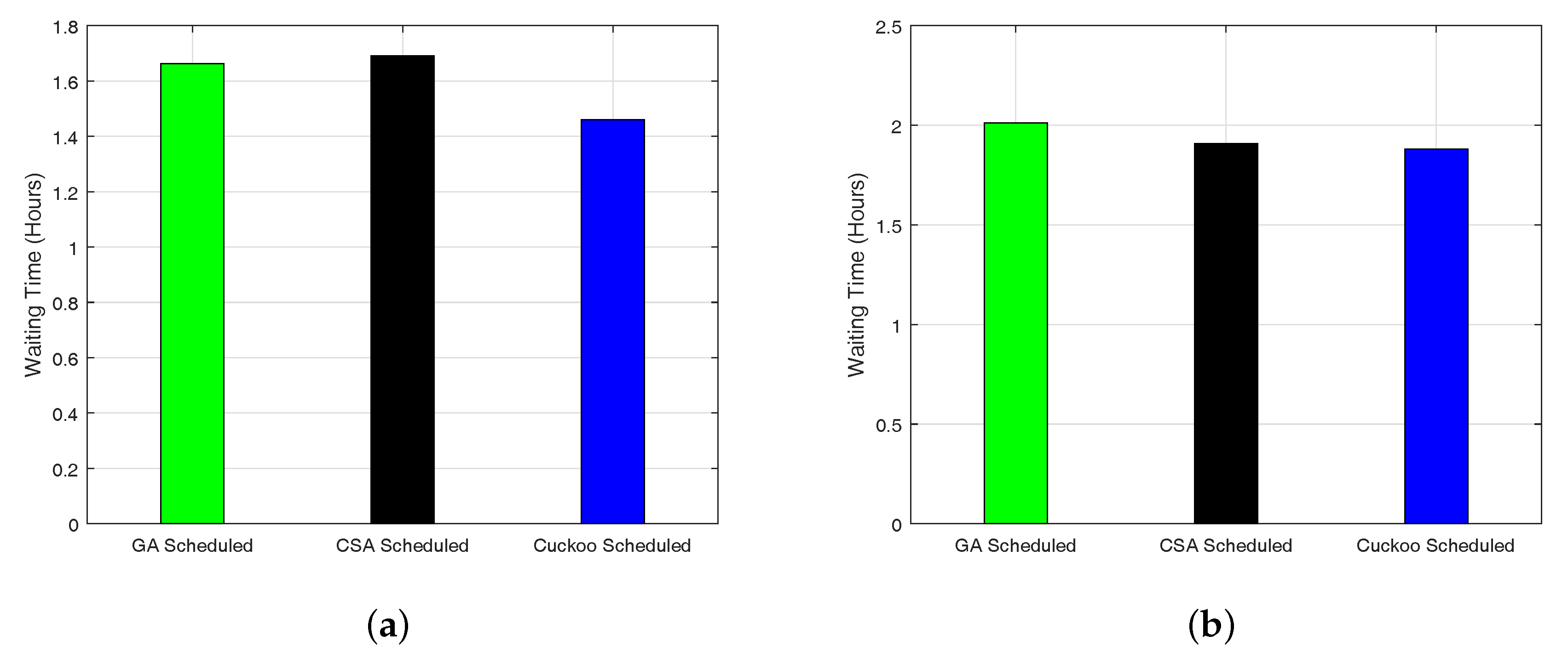
While decreasing the cost and PAR, the waiting time increases, which is shown in Figure 15a,b. However, our proposed scheme tries to minimize the user waiting time. It shows that there exists a tradeoff between electricity cost and user waiting time, and the results are explained in Table 6 and Table 7 for single and multiple smart homes, respectively. However, our proposed scheme achieves the desirable tradeoff between electricity cost and user waiting time. The waiting time of non-deferrable appliances is zero because these appliances may not be interrupted or shifted to any other time slot. Interior lighting, which is turned ON from the 18th–24th h and the length of operation of 6 h, and refrigerator, which is turned ON for 24 h, are parts of the non-deferrable appliances. Therefore, there is no waiting time for non-deferrable appliances.

From the simulations, it is concluded that GA is superior for obtaining the maximum number of the population due to the high convergence rate. GA is the oldest algorithm, which is used to search for the optimal solution. On the other hand, CSOA also shows high performance for the maximum number of the population. The main reason for the high performance of CSOA is that there are fewer parameters to be fine-tuned in CSOA than GA.

7. Conclusions and Future Work

With the invention of the smart grid, DSM and DR are the key enabling technologies for the equilibrium of electricity demand and electricity supply, which both enhance the stable operation of the electric grid and minimize the electricity cost for end consumers. In this paper, a meta-heuristic-based scheduling scheme has been proposed for the home appliance scheduling problem using GA, CSA and CSOA under two pricing schemes, RTP and CPP, for HEMS in DSM. The main targets of our study are to minimize electricity cost, PAR and user waiting time. The performance of our proposed scheme was evaluated via implementing it on a single smart home and a smart building comprised of thirty smart homes. Additionally, ESS is integrated for more efficient and reliable operation of the electric grid and electricity cost reduction. Feasible regions are also calculated for single and multiple smart homes using RTP and CPP signals, which demonstrate the effect of appliance scheduling on electricity cost with electricity consumption and user waiting time.

The results illustrate that the proposed scheme is able to schedule the electricity load from high price hours to low price hours while considering the minimum user waiting time and minimum PAR. The electricity cost is more reduced with the integration of ESS. Furthermore, our proposed scheme using CSOA shows supremacy in terms of cost and PAR minimization, while a desirable trade-off between electricity cost and user waiting time. The performance of CSOA is superior to CSA and GA because CSOA spent the maximum time on the global solution instead of the local solution, and there are fewer parameters to be fine-tuned than GA.

In the future, investigating other heuristic techniques for cost and PAR minimization is another direction of our research. We will also integrate a micro-grid (the user can produce electricity via RES) in HEMS for reduction of the load burden on the electric grid and electricity bill minimization for residential consumers.