A Security Level Classification Method for Power Systems under N-1 Contingency

1
Key Lab of Power Electronics for Energy Conservation and Motor Drive of Hebei Province, Yanshan University, Qinhuangdao 066004, China
2
Weixian Power Supply Subsidiary, State Grid Hebei Electric Power Co., Ltd., Weixian 056800, China
3
School of Electrical, Mechanical and Mechatronic Systems, University of Technology Sydney, Ultimo, NSW 2007, Australia
*
Author to whom correspondence should be addressed.
Energies 2017, 10(12), 2055; https://doi.org/10.3390/en10122055
Submission received: 7 November 2017
/
Revised: 30 November 2017
/
Accepted: 1 December 2017
/
Published: 5 December 2017
Abstract
:Security assessment is crucial for the reliable and secure operation of power systems. This paper proposes a security level classification (SLC) method to analyze the security level of power systems both qualitatively and quantitatively. In this SLC method, security levels are graded according to a comprehensive safety index (CSI), which is defined by integrating the system margin index (SMI) and load entropy. The SMI depends on the operating load and the total supply capacity (TSC) under N-1 contingency, and the load entropy reflects the heterogeneity of load distribution calculated from entropy theory. In order to calculate the TSC under N-1 contingency considering both of the computational accuracy and speed, the TSC is converted into an extended conic quadratic programming (ECQP) model. In addition, the load boundary vector (LBV) model is established to obtain the capacity limit of each load bus, and thus detect potential risks of power systems. Finally, two modified practical power systems and the IEEE 118-bus test system are studied to validate the feasibility of the proposed SLC method.
1. Introduction
Along with the continuous urbanization in China, the scale of regional power systems keeps on increasing, which brings a great challenge to guarantee the secure and reliable operation of regional power systems [1,2]. To meet this challenge, it is extremely important to study power system security under both normal and faulty conditions so as to allow system operators to take proper control measures when system security levels become low.
Traditional power system security analysis involves voltage stability [3,4], rotor angle stability, topological structure vulnerability [5], risk evaluation [6,7], extreme contingencies [8], etc. To accurately and efficiently assess power system security, large amounts of machine learning tools such as decision trees [9], extreme learning machine [10], and support vector machines [11] provide promising solutions. To alleviate the high computational complexity in these methods, several other technical measures, such as probabilistic neural network classifier [12] and important sampling methods [13], were introduced. However, the success of security assessment relies on the training set, which is determined by the performance of pattern classifiers. Furthermore, these obtained security levels are classified qualitatively rather than quantitatively. In recent years, much attention has been drawn to the cyber security issue in power system. Reference [14] proposes a security-oriented cyber-physical contingency analysis (SOCCA) method to plan for accidental contingencies and malicious compromises simultaneously. To identify critical substations and other “nightmare” hypothesized combinations for security protection planning, an impact analysis of critical cyber assets is introduced in [15] for substations which can capture historical load and topology conditions. In [16], two potential coordinated cyber-physical attacks (CCPAs) are presented and the adversary’s required capability to construct them is analyzed. To investigate the impacts of the cyber-contingency on power system operations, a simplified co-simulation model is proposed in [17].
As mentioned above, many security issues have been reported and discussed in the literature, but the security level classification (SLC) problem of power systems has not received much attention. Classification of security levels of the power system will enable operators to understand the system security levels in a straightforward way. For power systems with lower security levels, it is extremely important to monitor the power system in real-time and to identify potential system risks in a timely manner, preventing cascading failures and large-scale power outages. In this regard, the online module for power system static security assessment is implemented in [18]. To minimize the load-shedding or maximize the restoration of the unserved loads, a simulation framework is introduced in [19] to provide system snapshots during cascading failures. In [20], the authors proposed a set of security level classification (SLC) methods from the perspective of the static security and supply capacity of power systems, but the classifying principles and relevant classification factors need to be further improved.
Existing studies on power system security level mainly focus on two different aspects, which are the transmission network structure that connects generators and loads [21], and the operational states (i.e., levels of demand along with generation/load distribution and power flow). The first aspect of study calculates the maximum loadability by increasing the load level until a voltage, current, or voltage stability limit is reached in a power flow model [22]. Continuation power flow (CPF) is one of the most promising approaches in such studies. To find the equilibrium states through the entire loading range of an autonomous microgrid, the CPF method is illustrated and applied in [23]. In addition, a simulation method is proposed to compute the available load supply capability (ALSC) in [24]. But these methods often need very long computing time and will be inefficient for large-scale power systems. In [25], a new method is introduced to obtain the maximum load point of power systems based on the load flow method with optimal multiplier in rectangular coordinates. However, the method may bring a big error and certain random results, owing to the adoption of a specific load increase pattern. The second aspect of study emphasizes the optimal adjustment and matching between generation and load under various constraints [26,27], which is regarded as an optimal power flow (OPF) problem. In order to reduce the computational burden, linear programming (LP) is usually adopted to solve on the relevant DC power flow problem, which cannot handles all operational information with its simplified power flow equations. If all the AC power flow constraints are considered in the optimal model [28], the results will be more accurate than the simplified DC power flow approach, however, this alternative approach needs a lot of computing time and cannot be implemented online.
In this paper, total supply capacity (TSC) considering N-1 contingency is calculated to obtain the assessment indices which can reflect the security level of power systems [29], and the basic principles of SLC method in [20] are further developed into a systematic and complete SLC method. Key contributions of this paper are highlighted below:
- The proposed SLC method can assess the security level of power systems both qualitatively and quantitatively.
- Both of the power system structure and operational states are considered in the definition of comprehensive safety index (CSI) to evaluate power system security levels, where different indices, such as system margin index (SMI) and load entropy, are integrated. This will prevent any biased evaluation based only on one aspect of system structure or operational states. In addition, the defined load boundary vector (LBV) can detect the weakness in power systems and thus provides valuable reference for system operators to prevent any potential risk.
- Extended conic quadratic programming (ECQP) model is adopted to calculate TSC, where AC power flow is computed with higher precision at a reasonable polynomial computing time.
The rest of this paper is organized as follows: Section 2 presents the calculation methods for TSC and LBV. Section 3 describes the detailed classification principles for security levels of power systems. Section 4 validates the effectiveness of the proposed method through case studies on two modified practical power systems and the IEEE 118-bus test system. Section 5 gives some concluding remarks.
2. Calculation for TSC and LBV
According to the definitions of TSC and available supply capacity (ASC) in [30], the TSC can be described as the maximum supply load of power system. The ASC is equal to the difference between the TSC and existing load, and the value of ASC can be used to evaluate system ability to withstand load increment or fluctuation. The larger the value of ASC is, the more robustness the overall system is. In this section, to obtain the security level of a power system under N-1 contingency, TSC is calculated by converting into an ECQP model, and the corresponding capacity limit of each load node is obtained by the LBV model.
2.1. Contingency Screening
For a large-scale power system, calculating all the TSC values under N-1 contingency may be time-consuming and computationally intensive. Actually, among all the contingencies, there might be only one contingency or few contingencies corresponding to the minimum TSC. If these contingencies can be identified beforehand, it will significantly reduce the computational complexity.
The maximum network flow problem is to calculate the maximum transmission from a source node to a sink node considering the constraints of network topology. Similar to [31], the total maximum network flow of power system is adopted here, and it can be defined as the maximum total supply of active power from all generator nodes under DC power flow. To screen the contingency causing the worst effect on the TSC value for the purpose of reducing computational complexity, the system performance index (SPI) is defined as follows:
where and denote the total maximum network flow of a power system in normal operation and under the contingency i, respectively. G and L are the sets of all generation nodes and all load nodes, respectively; stands for the maximum supply of active power flow from generation node g to load node l, which is calculated by the Ford-Fulkerson algorithm considering the DC power flow constraints, and the Ford-Fulkerson algorithm is summed up in [32].
2.2. TSC Calculation under AC Power Flow
As indicated in the TSC definition mentioned before, the TSC refers to the maximum acceptable load of the power system, which can be obtained by optimizing the sum of all bus loads under the corresponding operation constraints. In this paper, the TSC is calculated by nodal injection powers considering AC power flow. To convert the TSC calculation model into the cone programming (CP) problem, the bus types of power systems are specially treated as following. If a bus comprises both the generation and the load, then a transmission line will be added between the generation and the load to divide the bus into a generation bus and a load bus. The resistance and reactance of added transmission lines are very small, which will not influence the calculation result. After the special treatment, all loads of the power system are not in the same buses with generation, and the injection power of each load bus is equal or less than zero. Thus, the TSC calculation problem considering AC power flow can be expressed as:
where D is the number of load buses; Pi is the injection power of load bus i.
Meanwhile, the nodal injection power constraints (4) and (5), voltage magnitude limits (6) and maximum permissible line current carrying capacity (7) are considered as follows:
where Gii, Bii, Gij, Bij are the self-conductance, self-susceptance, mutual conductance and mutual susceptance in the node admittance matrix, respectively; N(i) is the set of buses connected to bus i; and are the maximum injection active power and reactive power of bus i; and are the minimum injection active power and reactive power of bus i; Vi, Vj and θij are the voltage magnitude of bus i, j and the voltage angle difference between buses i and j, respectively; Vimax and Vimin are the maximum voltage limit and the minimum voltage limit of ith bus, respectively; Iij and Iimax are the current magnitude and the maximum current limit, respectively; , , , ; gij and bij are the series conductance and susceptance in the π equivalent model and bshij/2 is the 1/2 charging susceptance in accordance with line ij.
2.3. ECQP Model
In the CP problem, the objective function must be a linear function of decision variables, and its feasible region should be defined by linear equality/inequality constraints, and/or the second-order cone or a rotated cone inequality constraints. Therefore, in order to convert the TSC calculation problem under AC power flow into the ECQP model, new variables are defined as follows [33]:
In terms of these new variables, the nonlinear objective function can be expressed as:
Meanwhile, to complete the formulation in terms of the new variables, the injection power constraints of each node (10) and (11), voltage limits (12) and line current limits (13) are rewritten as:
According to (8), the new variables are constrained by the rotated quadratic cone as (14):
The variables Yij and Zij in (8) are defined for each transmission line. It is obvious that the new variables meet the requirement in (14). Equations (9)–(14) are equivalent to the original problem, and they meet the requirement for the linear objective function and equality/inequality constraints. Equation (14) makes the voltage decision variables form the Cartesian product of rotated cones, which implies that the search space is limited by convex cones.
In this paper, the ECQP model is solved by MOSEK [34], which is based on the interior-point (IP) algorithm. Thus, Equation (14) is modified to (15) for meeting the relevant requirement of MOSEK, and this modification does not change the feasibility and optimality of the obtained solution although the searching space is expanded:
Actually, when constraint (14) is replaced by (15), the linear objective function (9) can only achieve its maximum at its boundaries, which are defined by (14) and other linear constraints in (10)–(13). Therefore, this relaxation of constraint (15) still gives the same optimal solutions for (9)–(14). Once optimal solutions are obtained, the bus voltage magnitudes and angles can be calculated by (16) and (17):
2.4. Load Boundary Vector
The TSC describes the overall limitation of the supply capacity for power systems, whereas it cannot provide the capacity limit of each load bus. If the capacity limit can be calculated, it would be of great importance for the system operators to analyze the security margins of power systems. Besides, it is worth noting that for any particular value of TSC, there may exist multiple load operational points corresponding to this TSC (i.e., multiple solutions exist). Hence, the load boundary vector (LBV) is proposed to solve this issue, which can be obtained by optimizing the maximum injection power of each load bus under the constraints of TSC. The optimization objective is expressed as:
where λi is the maximum load that can be connected to load bus i when all the operational constraints are satisfied, and the LBV can be denoted by .
The nodal injection power of each generation bus is the same with the power generation distribution corresponding to TSC:
where Pg is the injection power of generation bus g; is the injection power of generation bus g under the TSC.
Similar to the constraints (4)–(7) of TSC model, the injection power limits (20) and (21), line current carrying capacity (22) and voltage magnitude (23) are expressed as:
The LBV represents the capacity limit of each load bus when the power system is under the TSC condition. The numerical values of components in this vector are different from the rated capacities of load buses which are decided by the transformers. Actually, due to power system structure and various operation constraints, some load buses cannot reach its rated capacity. With the LBV, the system operators can know the capacity limit of each load bus and identify load buses with actual capacity limit less than rated capacity, namely fragile load buses. The LBV is also used to obtain the valid load ratio in the following section.
3. Security Levels Classification for Power System
3.1. General Idea
In order to classify the security level of power systems, this paper mainly focuses on the power system structure and operational states. Potential risk of the power system is identified based on N-1 contingency test for the given system structure. For insecure power systems which do not meeting the N-1 contingency test, the severity of potential risk is rated according to load shedding and operating constraint violation. If a load shedding occurs, the security of the power system is regarded as the worst risky level. Otherwise, if the operating constraint violation occurs, the security of the power system is regarded as the less risky level. For power systems satisfying the N-1 contingency test, i.e., secure power systems, the comprehensive safety index (CSI) which combines system margin and disequilibrium load distribution (load entropy) is proposed. From the values of this CSI, the security of the power system can be further divided into different levels. The flowchart of the SLC method of power systems is shown in Figure 1.
3.2. SLC for Insecure Power Systems
Static security analysis refers to applying N-1 criterion to simulate the contingency of electrical components such as transmission lines and generators one by one. It aims to detect whether the load loss or operation constraint violation occurs. In order to depict the severity of load loss, the rate of load loss (PLloss) is defined as [20]:
where PLiloss is the load loss of node i after N-1 contingency; PLj is the load of node j at normal operation mode; D is the number of load nodes and m is the number of losing load nodes; αi is the load level factor (0 < αi < 1) determined by the load level of load node i.
When there exists a transmission line overloading without losing load after N-1 contingency, the following definition of index (PIk) can describe the severity of line overloading:
where β is the number of transmission lines exceeding their limits after N-1 contingency; and are the line active power flow and line capacity limit, respectively.
The index PIk can reflect the severity of line overloading after one component outage. However, it fails to describe the overall severity of the power system after all N-1 contingencies. For this reason, the danger index (DI) is defined as:
where NB is the number of components that cause lines overloading during N-1 contingency.
For the secure power systems, further work should be performed to analyze the security level, and this paper puts more emphasis on the SLC of power systems meeting N-1 contingency test.
3.3. SLC for Secure Power Systems
3.3.1. System Margin Index
Load is recognized as one of the most important variables for power systems. When the power system is in normal operation state, the degree of load increment or fluctuation, which can be tolerated or permitted by the power system, is generally adopted to reflect the security level of the power system.
Reference [35] gives the following definition with respect to system margin: the ratio between the actual maximum surplus power capacity and the actual load. The maximum surplus power capacity can be described by the difference between the TSC and the actual load. In this paper, similar to the ASC proposed in [31], the system margin index (SMI) is defined as:
where is the sum of all loads at normal operation state.
Equation (27) contains two influencing factors of SMI. One is the TSC and it reflects the maximum supply load of power system; the other is the real-time demand level. Larger SMI shows that the system can withstand greater load increment or fluctuation.
3.3.2. Load Entropy
The concept of entropy is derived from thermodynamics. Entropy is a measure of the chaos and disorder of the system. The less disorder the system is, the greater the entropy is. Conversely, the higher disorder of the system corresponds to the smaller entropy. In order to reflect the heterogeneity of load distribution in the power system, this paper proposes a concept called load entropy based on the entropy theory. The valid load rate of node i is expressed as:
where is the real power load of node i, and is the limit capacity of load node i obtained by LBV. ηi is the valid load rate, which can reflect precisely the load level of load node i, compared to the traditional load rate obtained with the ratio between actual load and rated capacity.
In an attempt to obtain load entropy, M successive intervals are defined as [0, u), [u, 2 × u), …, [(M − 1) × u, M × u), and it is assumed that valid load rates of all loads are in the interval [0, M × u). lk denotes the number of loads, whose valid load rate ηi falls within the k-th interval [(k − 1) × u, k × u), and the probability P(k) can be obtained by the valid load ratio of a randomly selected load in the k-th interval [(k − 1) × u, k × u):
Combine (28) and (29), and load entropy can be defined as follows:
where C is a constant. From (30), it can be observed that the load entropy provides an average measure for the heterogeneity of load distribution. Two extreme cases are the minimal and maximal values. When all the valid load ratios of loads fall in the same interval, the load entropy is zero, which stands for the most ordered status of load distribution.
3.3.3. Comprehensive Safety Index
To take the system margin and heterogeneity of load distribution into account in the SLC method of the power system, this paper presents a comprehensive safety index (CSI):
CSI is determined by two factors. One factor is the SMI. The larger the SMI is, the more secure the power system is. Another factor is the load entropy. A greater H value indicates a more unbalanced load distribution, which will reduce the security level of the power system.
CSI represents the comprehensive security of the power system. The indices of SMI and load entropy (H) reflect the security level of the power system from different perspectives. The SMI is a measure of the overall security level of the power system, while load entropy (H) portrays the distribution of each load.
3.4. SLC Principles
According to the static security analysis and the proposed indices, the security level of a power system is divided into five grades from high to low. Threshold values α and β (α > 0, β > 0 and α > β) are selected to determine second and third security levels, and they should be set based on the past experience of system operators and operation conditions of practical power systems. In this paper, we choose the CSI values under annual average load and annual peak load as the α and β values, respectively, because the annual average load and annual peak load are important characteristics of load distribution and can also reflect the most ordered load status. The values of α and β represent that the power system will reach its capacity limit with (1 + α) or (1 + β) times of current load level if all load nodes have the same load rates. Further details are given in the paragraphs below.
Grade I: CSI > α
It indicates that the security level of a power system is high, and the power system can withstand load growth in a large range based on current load level.
Grade II: β < CSI < α
It indicates that the security level of a power system is normal, and the power system can withstand load growth in a small scale based on current load level.
Grade III: 0 < CSI < β
It indicates that the security level of a power system is low, and a little load growth may result in line overload or loss of load.
Grade IV: DI > 0
It indicates that the power system would lead to line overload on the occasion of N-1 contingency test. There exists a security risk and system operators should take timely measures to guarantee the secure operation of the power system.
Grade V: PLloss > 0
It indicates that the power system would lose load when the N-1 contingency test is carried out. The power supply-demand balance cannot be achieved with load loss.
4. Case Studies
4.1. Two Modified Practical Power Systems
4.1.1. Basic Data
Two modified practical power systems (System A and System B) are studied in this paper. System A is shown in Figure 2, where a square box indicates the generator node, and a circle indicates the load node. This system has five generators, 13 transformer substations and 32 lines with the voltage level 220 kV. The capacity of generator U1 is 400 MVA, and other generators are 300 MVA. The transformer substation S13 connects to the 500 kV network with a maximum supply capacity of 1500 MVA.
4.1.2. Simulation Results and Analysis
Line outage analysis is carried out for System A based on the data of representative days. System A can operate regularly without line overload and load loss. However, if fault of line L3, line L4, line L5 or line L6 occurs, it will result in the outage of generator U2, U3, U4, and U5. In this paper, the method in [20] is applied to check the generator outage, and the outage of transformers at substations is not taken into account. The detailed analysis is given as follows:
1. Critical contingency screening
In order to reduce computational effort in the calculation of TSC under N-1 contingency, system performance index (SPI) is calculated, and SPI values of contingencies are ranked in descending order, which is presented in Table 1.
As Table 1 shows, only a few types of outages can affect the TSC, and most of line outages cannot influence the TSC value when the SPI value is less than 0.010. The SPI value of generator U1 contingency is the maximum, and the outage of generator U1 should be chosen to calculate the TSC firstly. Similarly, the TSC values of generator U4, U5, U2, U3 or line L5, L6, L3, L4 contingency need to be calculated secondly. Moreover, when an outage of line L23 or line L22 contingency occurs, the SPI value are 0.027 and 0.025, respectively, which also have an impact on TSC, because substations S9 and S11 are far from generator U1 and the 500 kV network, and the line L23 and line L22 are single transmission lines. After an outage at line L23 (or line L22), the power flow which is carried in line L23 (or line L22) will be transferred to line L22 (or line L23), resulting in thermal limit issue. Therefore, in order to ensure the reliability of power supply, other transmission lines or generators are needed to be connected to supply S9 and S11.
2. Results and analysis
The ECQP model is used to calculate the TSC under N-1 contingency test. The value of TSC is 2666 MW and the network loss is 32.14 MW. Table 2 shows the solution corresponding to TSC, including load active power of each substation and voltage at each bus. All the bus voltages meet the requirements of voltage limit. In order to verify the accuracy of AC power flow calculated by the ECQP model, the real powers in Table 2 obtained from the ECQP model are used in the Newton Raphson (NR) algorithm to calculate the AC power flow. Comparing the two methods, the results of the voltages are almost the same and the maximum error percentage is 0.003862%. It turns out that the ECQP model can be applied to calculate the AC power flow accurately. The consistency of results obtained by the two methods also verifies that the change from Equation (14) to Equation (15) does not influence the solution of the original problem.
Because the optimization model has been transformed into a series of linear formulations, the searching space for decision variables is constrained in the convex cone. It can significantly shrink the optimization feasible domain and improve optimization efficiency. The simulation only takes 0.41 s, which is much less than using a heuristic method.
In contrast to the ECQP method and linear programming (LP) method for DC power flow [20], the corresponding results of the two methods are shown in Table 3. It can be seen that the difference of the TSC values is 34.24 MW, which can be neglected comparing to the TSC value 2700 MW obtained by LP method. In addition, the bus voltages corresponding to LP are obtained by NR algorithm with the input of LP load solutions, and some bus voltages cannot meet the voltage limit requirements. Voltage values of nodes 9, node 12 and node 13 are 0.9471 p.u., 0.9288 p.u. and 0.9312 p.u., all of which are lower than the minimum limit 0.95 p.u. Meanwhile, the network loss cannot be calculated by the LP model. Furthermore, the computing time of LP method with DC power flow is 0.39 s, which is close to the simulation time using ECQP model. Thus, the ECQP method under AC power flow can obtain more accurate optimization results than LP method with approximate calculation time.
3. Security levels classification
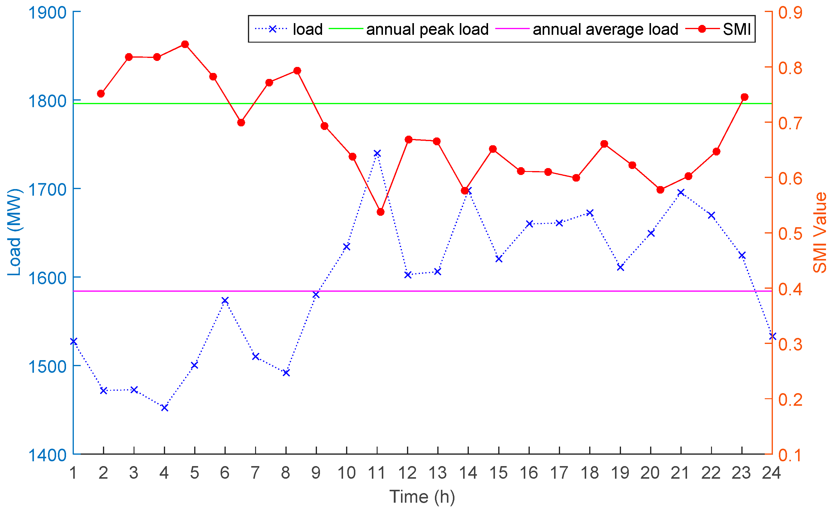
For the practical System A, the annual peak load and average load are 1796 MW and 1584 MW, and the α and β values are equal to 0.689 and 0.484, respectively. In this paper, a representative day load curve is selected to calculate the proposed indices and evaluate the security level of System A. Load data and corresponding SMI values are shown in Figure 3.
It can be seen that the SMI curve of System A is contrary to the change of load curve, which is determined by Equation (27). Furthermore, the load curve is greater than the annual average load during 10:00 to 23:00 on the representative day, while it is less than the annual average load at other time periods. At the load peak time 11:00, the SMI value is 0.637, which indicates that the TSC of System A is 1.637 times of current operation load.
To consider the influence of load distribution on security level of System A, the operation limit of each load node is calculated and the LBV is obtained as:
Most of the load nodes can reach its rated capacity in the power system, but the capacity limit values of load 9, load 12 and load 13 (339 MW, 304 MW and 336 MW) have a certain gap compared to their corresponding rated capacities (360 MW, 400 MW and 400 MW), owing to the security constraints of System A. By analyzing the structural characteristics of System A, it is found that the transmission lines connected to load node 9, load node 12 and load node 13 have longer distances, and the corresponding line impedances are big, which cause voltage drops at the receiving ends of the lines when large amount of power is transmitted. Therefore, it is necessary to reduce the capacity limit of load node to ensure voltage stability. Hence, the weakness of power systems, which is prone to violate voltage limit, can be identified by calculating the LBV.
Based on the operation load in each node and the given LBV, the load entropy index H can be calculated. Then the corresponding CSI values are obtained according to H and SMI values. These index values are shown in Figure 4. It can be seen that all the H values are between 0.13 and 0.18, which indicates that the load distribution of System A on the representative day is not homogeneous. Thus all the CSI values are less than SMI values. During the load valley time period from 2:00 to 4:00, the SMI values of System A are greater than other time periods, which results in the CSI values greater than threshold value α and the security level is in Grade I. On the contrary, at the peak load time 11:00, the SMI and H are equal to 0.537 and 0.144, respectively, thus the CSI value should be 0.470 and the security level is located in Grade III. This indicates that imbalanced load distribution can reduce the security level, and necessary monitoring of System A is needed to prevent any potential risk. Furthermore, the security level of System A is located in Grade II during other load time periods, which indicates that System A can withstand load growth in a small scale in most of the time of the representative day.
4. Comparison for different power systems
To illustrate that the SLC method can be applied to general systems, a comparison work has been done for two different power systems. System A is the one used in above section, and System B is part of another regional power system, whose parameters are omitted in this paper. Detailed analysis about System B is similar to System A and some details are not included in this paper to be concise.
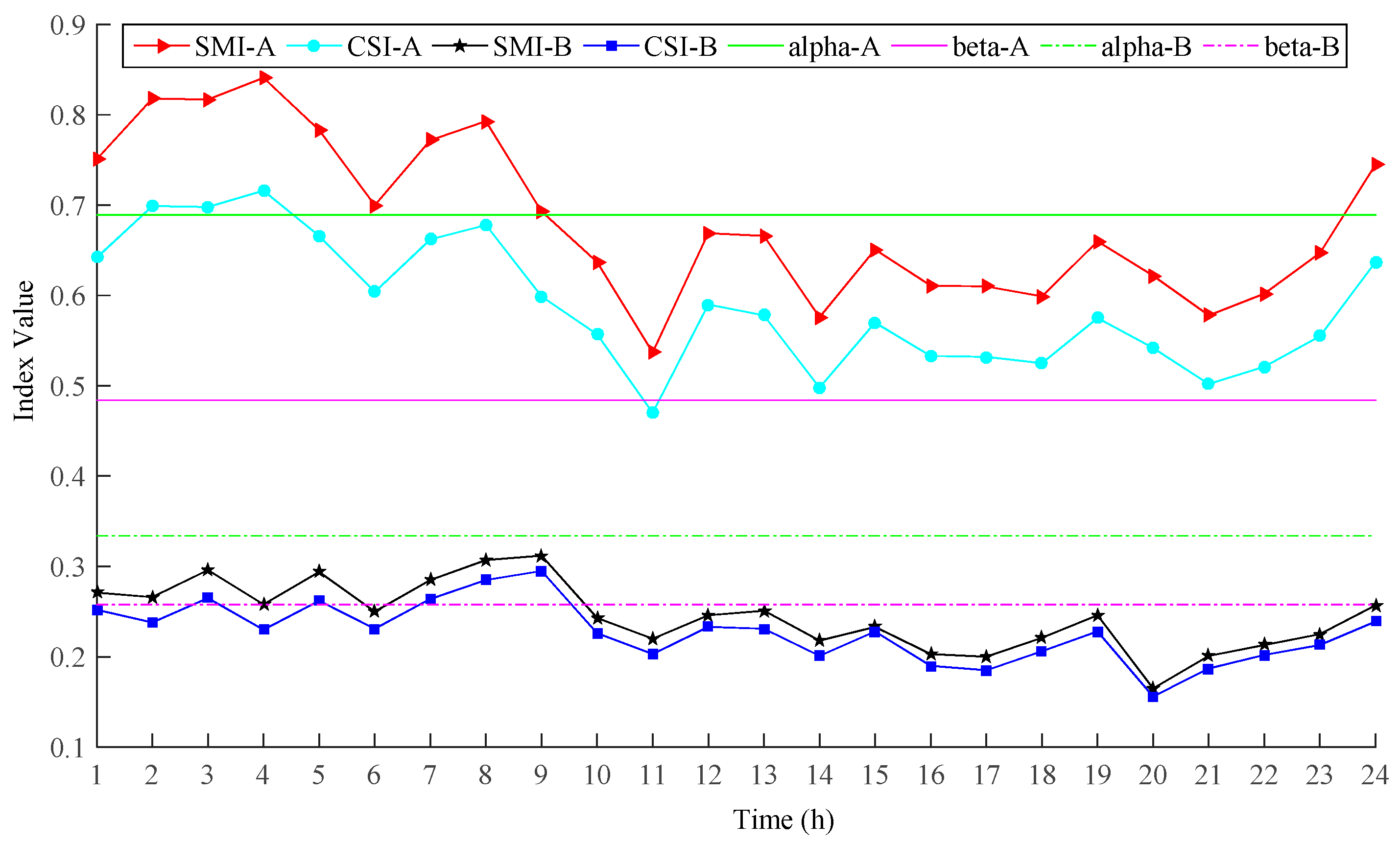
Figure 5 shows the comparison results of security levels for two different power systems. The α and β values of System B are equal to 0.334 and 0.258, respectively, and all the CSI values are lying in the interval [0.15, 0.30], which are significantly lower than System A. The security level of System B is in Grade II at 3:00, 5:00 and during 7:00 to 9:00, and it is located in Grade III during other time periods. Because System B has heavy industrial loads to be supplied, its SMI and CSI values are relatively lower. Therefore, the overall security level of System B is worse than System A. Meanwhile, the distance between different curves in Figure 5 can reflect the influence of imbalanced load distribution on security level, and the distance between the SMI curve and CSI curve of System B is much smaller than that of System A. This indicates that the load distribution of System A is more uneven than System B, and the imbalanced load distribution can reduce the security level.
4.2. The IEEE-118 Bus Test System
The proposed SLC method has been implemented on the IEEE 118-bus test system with the data from Matpower 5.0 [36]. During the N-1 contingency test, the load in node 117 will be lost due to an outage of the line 12–117. This indicates that the security level of the IEEE 118-bus test system should be in Grade V based on the proposed method, and the rate of load loss is 0.0024. Because the maximum transmission capacities of transmission lines are not given in the IEEE 118-bus test system, we assume that the maximum transmission capacity can meet the power transmission requirement and line overload will not occur.
In order to meet the N-1 contingency test, line 12–117 of IEEE 118-bus test system are improved to double circuit lines. After this modification, the SPI values of the modified IEEE 118-bus test system are calculated. The contingencies include 187 transmission lines and 54 generators, and the total number of contingencies is 241. Table 4 presents the SPI values of contingencies in the modified IEEE 118-bus system (“the generator in node 1” is abbreviated as “G1”, and the transmission line from node 1 to node 2 is abbreviated as “L1-2”).
It can be seen that the contingency severity of modified IEEE 118 test system mainly depends on the capacities of contingency generators, because all load nodes can be supplied by more than one branch and transmission line capacity will not be violated. Furthermore, the effectiveness of partial contingencies is the same, such as L9–10, L8–9 and G10, L110–111 and G111, which is determined by the network topology. After the contingency screening, the TSC values of partial contingencies listed in Table 4 are calculated based on the ECQP model instead of considering all 241 contingencies. Finally, the TSC of this modified IEEE 118-bus test system is chosen as 8749.37 MW considering the contingency at G89. The total operational load of the modified IEEE 118-bus test system is 4242 MW, and the SMI value is 1.06. This implies that if the load rates of all nodes are the same, then the modified IEEE 118-bus test system can withstand a load growth which equals 2.06 times of the current load level.
Similar to maximum transmission capacities of transmission lines, the maximum and minimum capacity limits of load nodes are not given in the IEEE 118-bus test system. In this paper, we assume that the maximum capacity limits of all load nodes are in equal proportion to current load level, which are assigned to be 0.99 times of maximum limits of all generation capacities. Ideally, the load capacity limits of all load nodes can be reached, and the load entropy equals 0 when all load nodes have the same valid load rates. However, due to the constraints of generation capacity and network topology, some load capacity limits of the LBV obtained by the model in Section 2.4 are less than the assigned values, and the corresponding results are shown in Table 5.
The load entropy index H is equal to 0.0939, which is calculated by current load level and LBV, and the CSI value is equal to 0.969. According to the above computation and analysis based on system structure and current load level, the modified IEEE118-bus test system can withstand a large range of load growth. Note that the annual peak load, annual average load, and the past experience of system operators are unknown, therefore, the IEEE 118-bus test system is mainly investigated to indicate that the SPI and other indices can be applied to large-scale power systems. For this reason, the security level of the IEEE 118-bus test system is not discussed in this paper.
5. Conclusions
This paper proposes a security level classification method to assess the security level of power systems. The TSC is calculated by the ECQP model, which is obtained from the TSC problem with AC power flow. The SMI and load entropy are integrated to define the CSI for the calculation of the security level of power systems. Furthermore, the LBV model is established and applied to detect the weakness of the power system. The feasibility and effectiveness of the proposed method have been validated by the case studies on two practical power systems and the IEEE 118-bus test system. Simulation results show that the adopted ECQP model can calculate the TSC and accurate AC power flow at the same time, while the computing time is close to LP method. Furthermore, the proposed SLC method and the corresponding security indices can be used to calculate and assess the security level of power systems, which provide a valuable reference for system operators.
Acknowledgments
This work is supported by the National Natural Science Foundation of China (61374098) and the National Natural Science Foundation of Hebei Province (F2016203507).
Author Contributions
All authors contributed equally to the work.
Conflicts of Interest
The authors declare no conflict of interest.
References
- Srivani, J.; Swarup, K.S. Power system static security assessment and evaluation using external system equivalents. Int. J. Electr. Power Energy Syst. 2008, 30, 83–92. [Google Scholar] [CrossRef]
- Kalyani, S. Pattern analysis and classification for security evaluation in power networks. Int. J. Electr. Power Energy Syst. 2013, 44, 547–560. [Google Scholar] [CrossRef]
- Zarate, L.A.; Castro, C.A.; Ramos, J.L.M. Fast computation of voltage stability security margins using nonlinear programming techniques. IEEE Trans. Power Syst. 2006, 21, 19–27. [Google Scholar] [CrossRef]
- Estebsari, A.; Pons, E.; Huang, T.; Bompard, E. Techno-economic impacts of automatic undervoltage load shedding under emergency. Electr. Power Syst. Res. 2016, 131, 168–177. [Google Scholar] [CrossRef]
- Bompard, E.; Napoli, R.; Xue, F. Extended topological approach for the assessment of structural vulnerability in transmission networks. IET Gener. Transm. Distrib. 2010, 4, 716–724. [Google Scholar] [CrossRef]
- Preece, R.; Milanovic, J.V. Risk-based small-disturbance security assessment of power systems. IEEE Trans. Power Deliv. 2014, 30, 590–598. [Google Scholar] [CrossRef]
- Feng, Y.; Wu, W.; Zhang, B. Power system operation risk assessment using credibility theory. IEEE Trans. Power Syst. 2008, 23, 1309–1318. [Google Scholar] [CrossRef]
- Lachs, W.R. Area-Wide System Protection Scheme against Extreme Contingencies. Proc. IEEE 2005, 93, 1004–1027. [Google Scholar] [CrossRef]
- Diao, R.; Vittal, V.; Logic, N. Design of a real-time security assessment tool for situational awareness enhancement in modern power systems. IEEE Trans. Power Syst. 2010, 25, 957–965. [Google Scholar] [CrossRef]
- Xu, Y.; Dong, Z.; Zhao, J. A reliable intelligent system for real-time dynamic security assessment of power systems. IEEE Trans. Power Syst. 2012, 27, 1253–1263. [Google Scholar] [CrossRef]
- Kalyani, S.; Swarup, K.S. Classification and assessment of power system security using multiclass SVM. IEEE Trans. Syst. Man Cybern. 2011, 41, 753–758. [Google Scholar] [CrossRef]
- Abdelaziz, A.Y.; Mekhamer, S.F.; Badr, M.A.L. Probabilistic neural network classifier for static voltage security assessment of power systems. Electr. Power Compon. Syst. 2011, 40, 147–160. [Google Scholar] [CrossRef]
- Perninge, M.; Lindskog, F.; Soder, L. Importance sampling of injected powers for electric power system security analysis. IEEE Trans. Power Syst. 2012, 27, 3–11. [Google Scholar] [CrossRef]
- Zonouz, S.; Davis, C.M.; Davis, K.R.; Berthier, R.; Bobba, R.B.; Sanders, W.H. SOCCA: A Security-Oriented Cyber-Physical Contingency Analysis in Power Infrastructures. IEEE Trans. Smart Grid 2014, 5, 3–13. [Google Scholar] [CrossRef]
- Ten, C.W.; Ginter, A.; Bulbul, R. Cyber-Based Contingency Analysis. IEEE Trans. Power Syst. 2016, 31, 3040–3050. [Google Scholar] [CrossRef]
- Deng, R.; Zhuang, P.; Liang, H. CCPA: Coordinated Cyber-Physical Attacks and Countermeasures in Smart Grid. IEEE Trans. Smart Grid 2017, 8, 2420–2430. [Google Scholar] [CrossRef]
- Cao, Y.; Shi, X.; Li, Y.; Tan, Y.; Shahidehpour, M.; Shi, S. A Simplified Co-simulation Model for Investigating Impacts of Cyber-Contingency on Power System Operations. IEEE Trans. Smart Grid 2017. [Google Scholar] [CrossRef]
- Kumar, R.S.; Mathew, A.T. Online static security assessment module using artificial neural networks. IEEE Trans. Power Syst. 2013, 28, 4328–4335. [Google Scholar] [CrossRef]
- Bompard, E.; Estebsari, A.; Huang, T.; Fulli, G. A framework for analyzing cascading failure in large interconnected power systems: A post-contingency evolution simulator. Int. J. Electr. Power Energy Syst. 2016, 81, 12–21. [Google Scholar] [CrossRef]
- Ma, L.; Jia, B.; Lu, Z.; Cao, L. Research on security classification of transmission network considering static security and real-time power supply capacibility. Trans. China Electr. Soc. 2014, 29, 229–237. [Google Scholar]
- Saric, A.T.; Stankovic, A.M. Model uncertainty in security assessment of power systems. IEEE Trans. Power Syst. 2005, 20, 1398–1407. [Google Scholar] [CrossRef]
- Michael, E.K.; Nicholas, G.M.; Costas, D.V. Maximizing power-system loadability in the presence of multiple binding complementarity constraints. IEEE Trans. Circuits Syst. 2007, 54, 1775–1787. [Google Scholar] [CrossRef]
- Díaz, G. Maximum loadability of droop regulated microgrids-formulation and analysis. IET Gener. Transm. Distrib. 2013, 7, 175–182. [Google Scholar] [CrossRef]
- Zhang, S.; Cheng, H.; Zhang, L. Probabilistic evaluation of available load supply capability for distribution system. IEEE Trans. Power Syst. 2013, 28, 3215–3225. [Google Scholar] [CrossRef]
- Hu, Z.; Wang, X. Efficient computation of maximum loading point by load flow method with optimal multiplier. IEEE Trans. Power Syst. 2008, 23, 804–806. [Google Scholar] [CrossRef]
- Kong, T.; Cheng, H.; Wang, J.; Li, Y.; Wang, S. United urban power grid planning for network structure and partition scheme based on bi-level multi-objective optimization with genetic algorithm. Proc. CSEE 2009, 29, 59–66. [Google Scholar] [CrossRef]
- Shu, H.; Hu, Z.; Liu, Z. Online evaluation of utmost power supply ability of urban power system and its application. Power Syst. Technol. 2008, 32, 46–50. [Google Scholar] [CrossRef]
- Xiao, J.; Liu, S.; Li, Z.; Li, F. Loadability formulation and calculation for interconnected distribution systems considering N-1 security. Int. J. Electr. Power Energy Syst. 2016, 77, 70–76. [Google Scholar] [CrossRef]
- Xiao, J.; Liu, S.; Li, Z.; Wang, C. Model of total supply capability for distribution network based on power flow calculation. Proc. CSEE 2014, 34, 5516–5524. [Google Scholar] [CrossRef]
- Xiao, J.; Li, F.; Gu, W. Total supply capability and its extended indices for distribution systems: Definition, model calculation and applications. IET Gener. Transm. Distrib. 2011, 5, 869–876. [Google Scholar] [CrossRef]
- Ju, W.; Li, Y. Identification of critical lines and nodes in power grid based on maximum flow transmission contribution degree. Autom. Electr. Power Syst. 2012, 36, 6–12. [Google Scholar] [CrossRef]
- Dwivedi, A.; Yu, X. A maximum-flow-based complex network approach for power system vulnerability analysis. IEEE Trans. Ind. Electron. 2013, 9, 81–88. [Google Scholar] [CrossRef]
- Jabr, R. A conic quadratic format for the load flow equations of meshed networks. IEEE Trans. Power Syst. 2007, 22, 2285–2286. [Google Scholar] [CrossRef]
- The MOSEK Optimization Tools Version 3.2 (Revision 8), Denmark. Available online: http://www.mosek.com (accessed on 8 August 2017).
- Power Grid Operation Standards. China. 2015. Available online: http://www.safehoo.com/Standard/Trade/Electric/201608/452584.shtml (accessed on 2 November 2017).
- The Matpower Simulation Package. 2016. Available online: http://www.pserc.cornell.edu/matpower/ (accessed on 6 November 2017).
Figure 1.
Flowchart of security level classification of power systems.
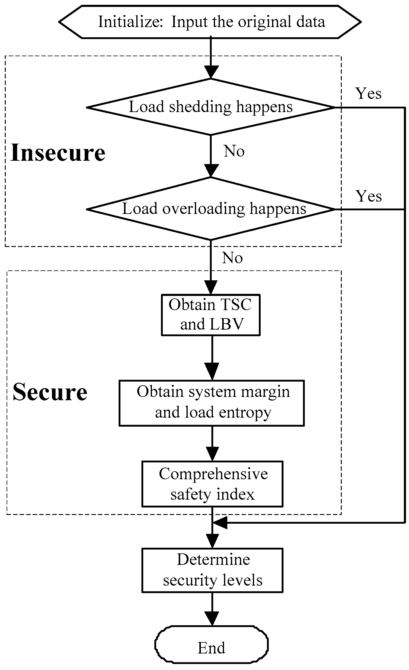
Figure 2.
System A.
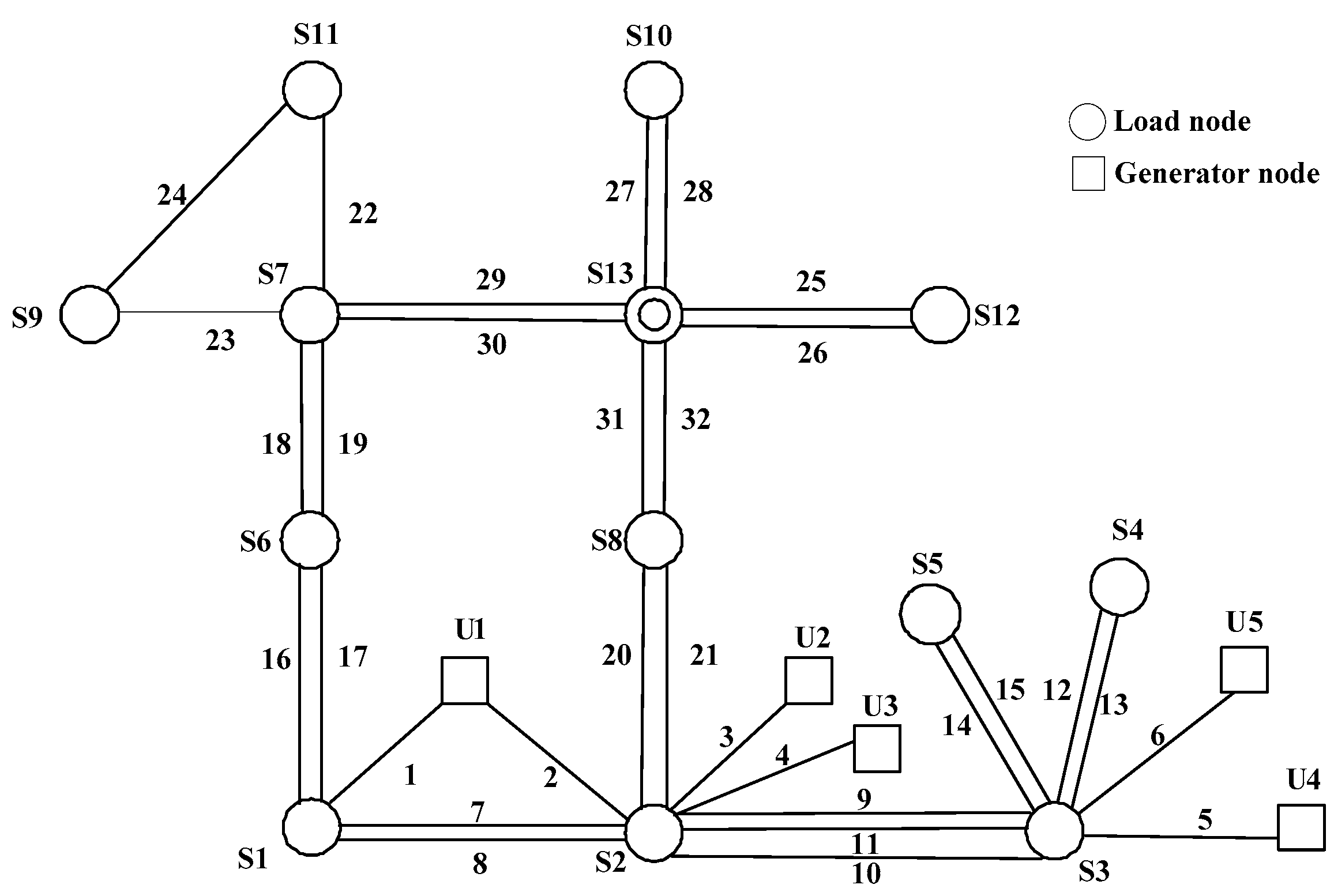
Figure 3.
Load and SMI values of System A.

Figure 4.
Index values and security level of System A.
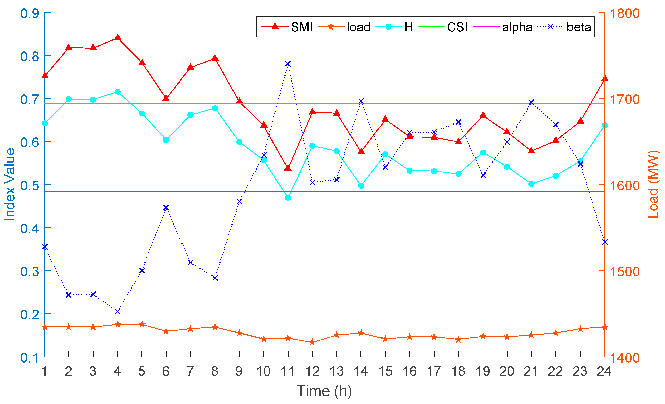
Figure 5.
Comparison results for the security levels of two different power systems.

Table 1.
SPI values of contingencies.
| Ranking | Contingencies | SPI |
|---|---|---|
| 1 | U1 | 0.129 |
| 2 | U4, U5, L5, L6 | 0.094 |
| 3 | U2, U3, L3, L4 | 0.093 |
| 4 | L23 | 0.027 |
| 5 | L22 | 0.025 |
| 6 | L26 | 0.009 |
| 7 | L27, L28, L29, L30, L14, L15 | 0.003 |
| 8 | L3, L4 | 0.002 |
| 9 | L9, L10, L24, L31, L32 | 0.001 |
| 10 | Others | Near to zero |
Table 2.
Extended cone quadratic programming (ECQP)-based solution accuracy verification.
| Substation No. | ECQP | NR | Error/% | |
|---|---|---|---|---|
| P | V/p.u. | V/p.u. | ||
| S1 | 281.94 | 0.980929 | 0.980949 | 0.002039 |
| S2 | 354.26 | 0.986529 | 0.986545 | 0.001622 |
| S3 | 354.16 | 0.986707 | 0.986726 | 0.001926 |
| S4 | 111.52 | 0.983807 | 0.983827 | 0.002033 |
| S5 | 111.33 | 0.983728 | 0.983748 | 0.002033 |
| S6 | 138.43 | 0.979961 | 0.979974 | 0.001327 |
| S7 | 249.15 | 0.981523 | 0.981537 | 0.001426 |
| S8 | 357.10 | 0.987960 | 0.987975 | 0.001518 |
| S9 | 180.56 | 0.963821 | 0.963822 | 0.000104 |
| S10 | 63.46 | 0.978277 | 0.978281 | 0.000409 |
| S11 | 63.38 | 0.978233 | 0.978237 | 0.000409 |
| S12 | 200.19 | 0.958037 | 0.958074 | 0.003862 |
| S13 | 200.28 | 0.964930 | 0.964936 | 0.000622 |
Table 3.
Comparison of solutions obtained by ECQP and LP.
| Substation No. | ECQP | LP | ||
|---|---|---|---|---|
| P | V/p.u. | P | V/p.u. | |
| S1 | 281.94 | 0.980929 | 274.69 | 0.982400 |
| S2 | 354.26 | 0.986529 | 149.81 | 0.989605 |
| S3 | 354.16 | 0.986707 | 360.00 | 0.989589 |
| S4 | 111.52 | 0.983807 | 120.00 | 0.986474 |
| S5 | 111.33 | 0.983728 | 120.00 | 0.986383 |
| S6 | 138.43 | 0.979961 | 154.39 | 0.980101 |
| S7 | 249.15 | 0.981523 | 25.00 | 0.978929 |
| S8 | 357.10 | 0.987960 | 300.13 | 0.989723 |
| S9 | 180.56 | 0.963821 | 235.07 | 0.947094 |
| S10 | 63.46 | 0.978277 | 100.00 | 0.965383 |
| S11 | 63.38 | 0.978233 | 100.00 | 0.965268 |
| S12 | 200.19 | 0.958037 | 400.00 | 0.929790 |
| S13 | 200.28 | 0.964930 | 360.91 | 0.931195 |
| sum | 2665.76 | -- | 2700 | -- |
Table 4.
SPI values of part contingencies.
| Ranking | SPI Values | Contingencies | Number of Contingencies |
|---|---|---|---|
| 1 | [0.07, 1.0] | -- | 0 |
| 2 | [0.06, 0.07) | G89, G69 | 2 |
| 3 | [0.05, 0.06) | G80, G10, L9–10, L8–9 | 4 |
| 4 | [0.04, 0.05) | G66, G65 | 2 |
| 5 | [0.03, 0.04) | G26, G100, G49 | 3 |
| 6 | [0.02, 0.03) | G25, G61, G59 | 3 |
| 7 | [0.01, 0.02) | G12, G54, L92–102, G46, G103, G92, G111, G31, L110–111, G40, G1, L110–111, L8–5, G42 | 14 |
| 8 | [0.073, 0.01) | L109–110, L71–73, L68–116, L86–87, L60–61, L110–112, and Other generators | 38 |
| 9 | [0, 0.005) | Others lines | 175 |
Table 5.
Results of load node capacities.
| Load Node | Assigned Capacity | Capacity in Obtained LBV | Difference (%) |
|---|---|---|---|
| 53 | 316.32 | 155.85 | 50.73 |
| 52 | 41.87 | 22.13 | 47.15 |
| 45 | 188.40 | 102.68 | 45.50 |
| 102 | 414.01 | 240.60 | 41.89 |
| 47 | 507.05 | 305.49 | 39.75 |
| 41 | 309.35 | 196.78 | 36.39 |
| 43 | 179.10 | 120.00 | 33.00 |
| 57 | 223.29 | 157.92 | 29.28 |
| 58 | 174.44 | 136.60 | 21.69 |
| 14 | 241.90 | 200.66 | 17.05 |
| 109 | 267.48 | 226.48 | 15.33 |
| 48 | 248.87 | 236.06 | 5.15 |
© 2017 by the authors. Licensee MDPI, Basel, Switzerland. This article is an open access article distributed under the terms and conditions of the Creative Commons Attribution (CC BY) license (http://creativecommons.org/licenses/by/4.0/).
Share and Cite
MDPI and ACS Style
Lu, Z.; He, L.; Zhang, D.; Zhao, B.; Zhang, J.; Zhao, H. A Security Level Classification Method for Power Systems under N-1 Contingency. Energies 2017, 10, 2055. https://doi.org/10.3390/en10122055
AMA Style
Lu Z, He L, Zhang D, Zhao B, Zhang J, Zhao H. A Security Level Classification Method for Power Systems under N-1 Contingency. Energies. 2017; 10(12):2055. https://doi.org/10.3390/en10122055
Chicago/Turabian StyleLu, Zhigang, Liangce He, Dan Zhang, Boxuan Zhao, Jiangfeng Zhang, and Hao Zhao. 2017. "A Security Level Classification Method for Power Systems under N-1 Contingency" Energies 10, no. 12: 2055. https://doi.org/10.3390/en10122055
Note that from the first issue of 2016, this journal uses article numbers instead of page numbers. See further details here.