Control Algorithms of Shunt Active Power Filter for Harmonics Mitigation: A Review


1
Department of Electrical and Electronic Engineering, Faculty of Engineering, Universiti Putra Malaysia, Serdang 43400, Selangor, Malaysia
2
Centre for Advanced Power and Energy Research (CAPER), Faculty of Engineering, Universiti Putra Malaysia, Serdang 43400, Selangor, Malaysia
*
Author to whom correspondence should be addressed.
Energies 2017, 10(12), 2038; https://doi.org/10.3390/en10122038
Submission received: 27 September 2017
/
Revised: 25 October 2017
/
Accepted: 30 October 2017
/
Published: 3 December 2017
Abstract
:Current harmonics is one of the most significant power quality issues which has attracted tremendous research interest. Shunt active power filter (SAPF) is the best solution to minimize harmonic contamination, but its effectiveness is strictly dependent on how quickly and accurately its control algorithms can perform. This manuscript reviews various types of existing control algorithms which have been employed for controlling operation of SAPF. Harmonic extraction, DC-link capacitor voltage regulation, current control and synchronizer algorithms are examined and discussed. The most relevant techniques which have been applied for each control algorithm are described and contrasted in an organized manner to identify their respective strengths and weaknesses. It is found that the applied control algorithms differ in two conditions: (1) the condition where harmonic current distortion is treated by the SAPF in the presence of non-ideal source voltage; and (2) the condition where multilevel inverter is employed as the circuit topology of SAPF.
1. Introduction
Proliferation of nonlinear loads resulting from technological advancements in the power electronics field has attracted the attention of researchers, engineers and others who are concerned about harmonic contamination in power systems. Notably, harmonic currents generated by nonlinear loads have caused many significant power quality problems to the power systems. Not only do they degrade the power factor (PF) performance of an operating power system, but they also cause other severe problems, which include overheating of equipment, errors in measuring instruments, failures of sensitive devices and capacitor blowing [1,2].
Therefore, in order to restrict activity of harmonic currents, IEEE standard 519 (the latest revised version is IEEE 519-2014 [3]) has been formulated. It is clearly stated in the harmonic standard that the total harmonic distortion (THD) for current should be at most 5%. Hence, the 5% current THD limit has always been the performance target that all researchers and designers are trying their best to achieve. In order to deal directly with the harmonic problems and to comply with the 5% limits, conventional passive harmonic filters are applied [4]. However, due to their major weaknesses of bulky sizes and fixed mitigation abilities, innovative and efficient harmonic mitigation tools known as active power filters (APFs) are developed to replace them. Besides, the development of APFs is also spurred by the emergence of power semiconductor switching devices such as insulated-gate bipolar transistors (IGBTs) and availability of powerful controllers such as digital signal processors (DSPs) [4].
Since the development of APFs, various authors have surveyed and reviewed them from different perspectives. An early literature survey was performed by Grady et al. [5], where they categorized the operation of active power line conditioners (APLCs) into time-domain and frequency-domain mitigation approaches, and highlighted the advantages and disadvantages of each mitigation approach. Next, Singh et al. [6] categorized a large number of reported APFs according to converter type, the applied topology, characteristics of the power system, control algorithms and designated applications. In [7], Peng presented a total of 22 power filter configurations which included basic power filters and all the possible combinations of the basic power filters named as hybrid power filters. The characteristics and suitable applications for each configuration were examined and compared in a concise manner. Another review focusing on classifications of APFs was conducted by El-Habrouk et al. [8] where the existing works on APFs were categorized according to the power rating of the operating power system, power circuit configuration, mitigation purposes (such as current harmonics, power factor, and unbalances), control algorithms employed, and reference current/voltage generation approaches. Brief discussions were provided for each category but the review is comprehensive, especially concerning the existing power circuit configurations of APFs.
In [4], Akagi reviewed the emerging APF field with a comparison to traditional passive filters, and clearly described its functions, and its classifications based on circuit configuration, overall control system and applications. A detailed literary review on control algorithms of APFs is presented in [9], where time-domain, frequency-domain, impedance synthesis, instantaneous power, DC-link voltage regulation, current reference following techniques are examined, contrasted and discussed. It is revealed that while some control algorithms offer some implementation advantages over the others, they all provide almost similar performance if the source voltage is ideal (undistorted). Besides, it is also found that some control algorithms will not work appropriately in the presence of non-ideal (distorted and/or unbalance) source voltages, and must be further modified when applied in practical environments. Additionally, there are several reviews such as [10,11] that compare the commonly applied control algorithms for the purposes of harmonic extraction and reference current generation in APFs. These reviews provide details on the working principle of each reviewed control algorithm and concisely highlight their respective strengths and weaknesses.
From the existing literature reviews [4,6,8], it is revealed that shunt-type APFs (SAPFs) are the most suitable to deal with harmonic current distortions. Additionally, they are also capable of improving the power factor (PF) performance [6,12,13] by reducing the reactive power burden on the power system, while mitigating harmonic currents. SAPFs were also found to be commercialized to fulfill customers’ demand in managing tough power quality problems which can occur in industrial and commercial environments. ASEA Brown Boveri (ABB) [14], Schaffner [15] and Schneider Electric [16] are three examples of the well-known companies developing SAPFs. Generally, the commercial SAPFs are developed for triple functions which include selective harmonic filtering, reactive power compensation and load balancing. They are designed for three-phase systems (three-wire or four-wire) and are available in different current ratings to suit different applications in both low-voltage and medium-voltage networks. Besides, they can dynamically adapt to changing grid and load situations, thus providing optimum compensation performance at all times. However, the applied controller topology for SAPFs may be different for each company. For instance, ABB active filters are controlled by a digital closed-loop controller which generates pulse-width modulation (PWM) pulses that drive the power modules [14]. Meanwhile, the operation of Schaffner active filters is managed by a digital controller integrated with a fast Fourier transform (FFT) analysis [15]. On the other hand, Schneider active filters are designed with two types of control schemes: a digital-based control scheme with FFT analysis and an analog-based control scheme (without FFT) named full spectrum cancellation [16].
The effectiveness of a SAPF is strictly dependent on the performance of its control algorithms [17]. To date, various control algorithms have been developed to control SAPFs under different operating environments. However, there is a general lack of published material providing a complete overview of the working principles of SAPFs and their control algorithms such that researchers and designers can grasp the basics of SAPFs and at the same time compare and evaluate various control algorithms in a subjective fashion. This manuscript aims to fill this gap.
SAPFs are available in four distinct forms which are categorized according to the circuit topology employed, namely standard inverter (either voltage source inverter (VSI) or current source inverter (CSI)), switched capacitor, lattice structure and voltage regulator [8]. Nevertheless, voltage source inverters are the most preferred for SAPFs due to their small physical sizes and low development costs [4]. Another unique characteristic of voltage source inverters that makes them ideal for SAPF implementation is their expandable nature to multilevel and multistep versions which greatly enhance their performance in harmonics mitigation [18]. Therefore, the discussion in this manuscript focuses solely on the case of VSI-based SAPFs.
This manuscript classifies various control algorithms which have been reported for VSI-based SAPFs (covering both standard two-level and multilevel inverters), and highlights their respective features. Control processes of SAPFs which include harmonic extraction, reference current generation, DC-link capacitor voltage regulation and current control are covered. In this manuscript, the control algorithms are described for three-phase SAPFs as the more general situation. Nevertheless, control algorithms that can be applied in single-phase SAPF are also highlighted and discussed.
The manuscript is organized as follows: Section 2 describes the typical control structure and working principle of SAPFs. Section 3 outlines and discusses exhaustively all the commonly applied control algorithms for operating SAPFs under ideal source voltage condition. Section 4 highlights the necessary modifications to the control algorithms for controlling SAPFs when subjected to unbalanced and/or distorted source voltages, and the available techniques. Section 5 describes the control algorithms for operating multilevel inverter-based SAPFs. Lastly, Section 6 concludes and highlights the most important findings of this review.
2. Control Structure and Working Principle of Shunt Active Power Filter
Figure 1 shows the overall circuit configuration of a typical voltage source inverter-based SAPF and illustrates its four main control algorithms. Generally, a SAPF is connected to a harmonic-polluted power system at the point of common coupling (PCC), between the voltage supply and a harmonic-producing load. The structure of a SAPF consists of two main elements, namely a standard two-level voltage source inverter and controller. Meanwhile, its controller involves four main control algorithms: (1) harmonic extraction (also known as reference current generation); (2) DC-link capacitor voltage regulation; (3) current control (also known as switching); and (4) synchronizer algorithms. The functions of all the elements in Figure 1 are highlighted as follows:
- (1)
- Harmonic Extraction Algorithm. This control algorithm operates by first taking the distorted load current signal from the harmonic-polluted power system, followed by isolation of harmonic and fundamental current components, and ends with the generation of a reference current signal . The generated reference current signal is used to govern the operation of the SAPF in reducing the harmonic distortion. Since its main purpose is to generate a reference current signal, hence it is also known as reference current generation algorithm.
- (2)
- DC-link Capacitor Voltage Regulation Algorithm. The control algorithm that takes the instantaneous DC-link capacitor voltage and compares it with a desired reference value. The resulting error is used to estimate the suitable magnitude of the instantaneous DC-link charging current . The estimated is the amount of needed to be drawn by the SAPF to regulate its switching losses so as to constantly maintain DC-link capacitor voltage at the desired reference value.
- (3)
- Current Control Algorithm. This is the control algorithm that takes the output of the harmonic extraction and DC-link capacitor voltage regulation algorithms to generate switching pulses for the controlling operation of the inverter so that it functions as a SAPF. It consists of a pulse-width modulator to generate the desired switching pulses and a local current control loop that ensures that the injection current is generated according to the reference current .
- (4)
- Synchronizer Algorithm. This control algorithm (commonly developed based on phase-locked loop (PLL) techniques) takes the source voltage signal and generates a synchronization angle/phase, so that injection current which is injected by the SAPF into the operating power system is correctly synchronized with the source voltage. It should be noted that certain SAPF controllers do not require explicit synchronization algorithms.
- (5)
- Voltage Source Inverter. This is a power converter which is systematically controlled to reproduce the reference current as injection current , at suitable magnitude. It is equipped with a DC-link capacitor (energy storage element) to compensate real power unbalance that occurs during dynamic operation of the SAPF and a filter inductor to minimize the ripples of injection current .
- (6)
- Harmonic-producing Load. This is a nonlinear load which injects a harmonic current into an operating power system via PCC. Switch-mode power supplies, arc furnaces, adjustable speed drive (ASD), and rectifiers are a few examples of practical loads that generate serious amounts of harmonic currents and reactive power in the power system. However, in simulation and laboratory evaluations, an uncontrolled bridge rectifier is most commonly applied, as it causes the worst harmonic current distortions [1,17,19]. Note that, the output of the bridge rectifier is normally connected to three types of loads: (1) series connected resistor and inductor (simply known as inductive load); (2) parallel connected resistor and capacitor (simply known as capacitive load); and (3) a single resistor (simply known as resistive load).
From Figure 1, assuming that the SAPF is not yet connected, the current flow in a harmonic-polluted power system can mathematically be expressed as:
where is the fundamental current and is the harmonic current generated by the harmonic-producing loads. Note that the source current in this case, is distorted due to addition of and has displaced away from the source voltage .
However, after connecting the SAPF at the PCC (as shown in Figure 1), there are two additional current flows in the harmonic-polluted power system: (1) injection current which is an opposition mitigation current injected by the SAPF into the harmonic-polluted power system to cancel out ; and (2) DC-link charging current which is a small amount of current drawn by the SAPF to regulate its switching losses and to maintain at constant level.
Hence, with the installation of a SAPF, Equation (1) can be re-written according to Kirchhoff’s current law (KCL) as:
To put it simply, the function of SAPF is to effectively recover the sinusoidal shape of , by injecting into the harmonic-polluted power system to cancel out contained in . This can simply be achieved by making equal to . In this manner, will eventually regain its sinusoidal characteristic and work in-phase with . Hence, Equation (2) can now be simplified as:
For better demonstration of the SAPF’s operation, theoretical SAPF waveforms in the situation where the harmonic-producing load is assumed to be a three-phase uncontrolled bridge rectifier feeding an inductive load, are illustrated in Figure 2.
3. SAPF Control Algorithms
The control algorithms of SAPFs are initially developed to operate SAPFs under the case of an ideal source voltage where the source voltage is assumed to be sinusoidal and balanced. This is because the main function of a SAPF is to mitigate harmonic currents generated by nonlinear loads, and a distortion-free source voltage is essential for the effective operation of a SAPF. In SAPF operation, the angular position of the source voltage is usually taken as the reference to coordinate the phase of its output injection current, so that it will work in phase with the operating power system [4,19,20]. Nevertheless, to fulfill practical needs, innovative modifications and improvements have been performed on the control algorithms so that SAPFs can be controlled to work effectively when subjected to non-ideal source voltage conditions (this will be discussed in Section 4). This section discusses the control algorithms which have been applied to operate SAPFs under ideal source voltage conditions.
3.1. Harmonic Extraction Algorithm
The extraction or detection of harmonic currents from the harmonic-polluted power line to generate the reference current signal by using a harmonic extraction algorithm is deemed the first and the most important operation stage of a SAPF’s control system [21,22]. Being the very first algorithm to operate in the controller, accurate and fast harmonic currents extraction result in proper and fast reference current generation which further controls the SAPF to efficiently reproduce the reference current signal as the desired injection current for harmonics mitigation. Basically, the algorithm utilizes a signal-processing function known as distortion identifier which takes the distorted load current signal and generates a corresponding reference current signal by isolating the distortion components from the fundamental component. To date, various harmonics extraction algorithms have been reported in the literature and their performances have been explored [9,10,11]. Generally, the existing algorithms are classified as time-domain, frequency-domain, and learning technique. Nevertheless, other modified versions of the aforementioned approaches are also available.
3.1.1. Time-Domain
Time-domain harmonics extraction approaches are based on the instantaneous derivation of reference current signals from harmonic-polluted sources. They are considered as the simplest harmonic extraction approaches, offering increased speed and fewer calculations as compared to their counterparts in the frequency-domain and learning technique categories. In time-domain, the most widely applied algorithms are synchronous reference frame (SRF) [17,23,24] and instantaneous power (pq) theory [1,11,21]-based approaches.
(1) SRF algorithm. Harmonics extraction based on the SRF (also as known as theory) algorithm is accomplished through a series of mathematical calculations of three-phase load current which is conducted in direct-quadrature-zero frames. Park-transform matrix is applied to convert three-phase load current in -frames to rotating -frames . However, only -frames involves in the extraction process. Here, the -frames are determined by the reference phase which is delivered by a synchronizer (particularly a PLL). In -frames, the fundamental component will appear as DC signal, and the harmonic components will appear as ripples. A low-pass filter (LPF) is commonly used to separate fundamental components and harmonic components [17,24]. Finally, the desired reference current is generated by using the extracted harmonic components via inverse Park-transformation. Figure 3 shows the control structure of a typical SRF algorithm.
This algorithm is applicable only to three-phase system with balanced and sinusoidal voltage waveform, and it experiences time delays in extracting the fundamental component.
(2) pq Theory algorithm. Harmonics extraction based on a pq theory algorithm is realized through a series of mathematical calculations of instantaneous power in a balanced three-phase system. The calculations are conducted in αβ-frames where the three-phase source voltage and load current signals are first transformed into αβ-frames via Clarke-transformation and are then applied to calculate the instantaneous active and reactive powers of the load. In αβ-frames, the fundamental component of the instantaneous power and will appear as DC signal, and the harmonic power components and will appear as ripples. Note that only active power needs to be filtered (commonly by LPF) to obtain the desired harmonic components [1,11]. Finally, the reference current is generated by using the extracted harmonic components via inverse Clarke-transformation. Figure 4 shows the control structure of a typical pq theory algorithm. Like the SRF algorithm, this algorithm is also applicable only to three-phase systems with balanced and sinusoidal voltage waveforms. It also experiences time delays in extracting the fundamental component due to the dependency on LPF.
3.1.2. Frequency-Domain
In the context of SAPF control strategies, frequency-domain harmonic extraction algorithms are based on Fourier analysis which involves either discrete Fourier transform (DFT) [25,26] or fast Fourier transform (FFT) [27,28] of the distorted current signals. From measurement of the distorted line current, the desired harmonic components are separated or isolated from the measured signals and are then reconstructed back in the time-domain to generate reference current signals. For effective harmonic mitigation, the switching frequency of SAPFs is kept generally at more than twice the highest harmonic frequency of the reference current signals [9,29]. Frequency-domain approaches are suitable for both single- and three-phase systems. The main disadvantage is that they require time to gather sufficient samples so that they can be processed in Fourier analysis [30]. Moreover, due to large computational burden it imposes, a really good and fast control processor must be considered, to ensure efficient performance of frequency-domain approaches.
3.1.3. Learning Techniques
Another method to extract the desired harmonic components is by using a learning technique. The available techniques in this category include optimization, and artificial intelligence (AI) approaches such as Genetic Algorithm (GA) and Artificial Neural Network (ANN). In SAPF applications, optimization algorithms have been applied in switched capacitor active filters to extract the harmonic components which are directly used to generate the switching pattern of the reference current [31]. However, the method tends to complicate computation, and degrade the dynamic response of the SAPF. Next, genetic algorithm (GA) has been incorporated to improve the convergence time [31]. However, GA techniques are complex, difficult to implement and they require a very long execution period [32].
Owing to the limitations of both techniques, ANN is applied to learn the characteristics of the harmonic-polluted distribution system so that a suitable reference current signal can be set to achieve an allowable level of harmonic distortion in the distribution system [9,11]. The ANN technique is constructed as a computational algorithm based on the structure and functions of biological neural networks. It requires a separate network to represent each harmonic frequency, which thereby increases the computation time. Nevertheless, further control-scheme modification has been performed on the conventional ANN technique (renamed as modified ANN) through a weights-updating algorithm [20,33], which speeds up extraction process and shortens the adaptation time. Figure 5 shows the control structure of a modified ANN algorithm.
In operation, the load current is first sensed and compared with an initial estimated current . Note that constant is the sampling rate, for digital implementation. The resulting error is processed by a weight updating algorithm to update the weight or the amplitude and of sine and cosine vectors. The iteration is repeated until = . Here, the sine vector which contains the fundamental current component will be taken and compared with to derive the reference current . This algorithm is applicable for both single- and three-phase systems. The main disadvantage is that a precise learning rate value is required by the algorithm to perform efficiently, normally obtained via a heuristic approach.
3.1.4. Other Algorithms
Control algorithms other than the three aforementioned categories of the harmonic extraction algorithms described above, are also available. These control algorithms are implemented by applying small changes to the aforementioned algorithms, and they provide simply better performance over their respective predecessors.
In the context of time-domain approaches, the modifications are mainly implemented to overcome the time delays exhibited by numerical filters. For the SRF algorithm, the modifications which have been implemented include replacement of LPFs with sliding window Fourier analysis (SWFA) which is renamed as with Fourier (F) [34,35], replacement of LPFs with wavelet approach [36], and simplification of overall control structure which is renamed as simplified SRF (SSRF) [17]. The work on both F and the wavelet algorithms are limited only to simulation study. Meanwhile, the work on SSRF is proven to work effectively in both simulation and practical environments and has achieved a significant performance improvement in both steady-state and dynamic environments. On the other hand, for pq theory algorithms, the reported modifications include integration of a fuzzy logic controller (FLC) [21], replacement of LPFs with sliding window Fourier analysis (SWFA) which is renamed as pq with Fourier (pqF) [37], and replacement of LPFs with an averaging algorithm which is renamed as enhanced pq theory [1]. The modifications that works on pq theory algorithms focus more on simulation studies but these studies provide a comprehensive analysis of both steady-state and dynamic environments.
Another modification work is on the ANN algorithm. From the modified ANN as shown in Figure 5, further changes have been implemented and even the control structure has been simplified. The algorithm is named as fundamental active current (FAC) ANN [22]. As compared to the modified ANN algorithm, the FAC ANN algorithm is reported to provide better performance in both steady-state and dynamic environments. However, the algorithm is only reported for single-phase systems and its main disadvantage of requiring a precise learning rate has not been addressed.
3.2. DC-Link Capacitor Voltage Regulation Algorithm
Another important control stage of a SAPF’s control system is to ensure constant voltage at DC side of the power converter via a DC-link capacitor voltage regulation process. Generally, DC-link capacitor voltage regulation is related to a voltage source inverter-based SAPF configuration where a DC capacitor is usually installed for energy storage. The voltage should remain constant in an ideal case, with no real power exchange between the SAPF and the AC network. However, this condition is not possible in practical environments due to power losses in the power converter as a result of conduction and switching activities. Therefore, DC-link capacitor voltage regulation is crucial in maintaining a constant voltage across the DC-link capacitor, and it must be maintained at a level which is high enough so that the SAPF is able to precisely inject the desired injection current back into the harmonic-polluted power system.
Basically, DC-link capacitor voltage is regulated by controlling the real power drawn by the SAPF throughout its switching operation. The voltage regulation process is said to have accomplished when the real power drawn by the SAPF is made equal to its switching losses. Therefore, in order to constantly the maintain proper function of SAPFs, the magnitude of the generated reference current must be suitably adjusted by manipulating the magnitude of a control variable known as instantaneous DC-link charging current signal (cf. Figure 1), so that a precise amount of real power can be drawn by the SAPF to compensate its potential losses. To date, various DC-link capacitor voltage regulation algorithms have been reported in the literature and their performances have been explored. They can generally be classified as direct voltage error manipulation [38,39,40] and self-charging [20,41,42]-based approaches. Nevertheless, other modified versions of the aforementioned approaches are also available [2,41].
3.2.1. Direct Voltage Error Manipulation Approach
Conventionally, the overall DC-link voltage is regulated via a direct voltage error manipulation approach where the difference (voltage error ) between overall DC-link voltage signal and its desired reference voltage is directly manipulated by either a proportional-integral (PI) controller [40,43,44] or a fuzzy logic controller (FLC) [38,39,45] as shown in Figure 6, to produce an estimated output which is assumed to be the main control signal for regulating the DC-link voltage. Note that is the sampling rate.
The PI technique (cf. Figure 6a) is more widely used due to its simple implementation features. The overall DC-link voltage can be regulated just by applying fixed values of proportional gain and integral gain . However, due to the use of fixed gain values, the PI technique is unable to work satisfactory under dynamic-state conditions. As a result, it performs with high overshoot [38,40,46] and large time delay [38,47,48] under dynamic-state conditions. This greatly degrades the effectiveness of SAPFs in mitigating harmonic currents. Besides, PI controller design requires a precise linear mathematical model which is difficult to obtain in nonlinear and time-varying systems [38,49,50] and thus the tuning procedure for the determination of optimal gain values can be very time-consuming [49]. Therefore, it is not worthwhile to allocate such a long time just to obtain a fixed gain value.
Owing to the weaknesses of the PI technique, the FLC technique was introduced. There are basically four processes in FLC operation, which starts with fuzzification, followed by fuzzy rule base and inference interpretation, and ends with defuzzification. In fuzzification stage, the numerical voltage error and change of error variables are converted into their corresponding linguistic representations, based on their respective fuzzy membership functions. Note that is the sampling rate. The shape of fuzzy membership functions can be in the form of triangular, trapezoidal, Gaussian, bell-shaped and sigmoidal functions [51,52]. Nevertheless, the most commonly applied membership functions are the combination of triangular and trapezoidal functions as they are famous for their simple implementation features and minimal computational efforts [45,50].
All input conditions will be processed by fuzzy inference mechanism to generate the most appropriate fuzzified output according to the designed fuzzy rule base table which composes a collection of simple linguistic “If A and B, Then C” rules. The most commonly applied inference mechanism is known as Mamdani-style inference mechanism [41,53,54] as it requires less complex computational process [49]. The generated fuzzified output is converted back to its corresponding numerical magnitude via defuzzification process. Most FLC systems use the famous centre of area (COA) or centroid defuzzification method [41,53,54] as they provide a good average feature in determining the best output result.
By incorporating the advantages of FLC, the performance of a SAPFs in terms of overall DC-link voltage regulation have been significantly improved [38,47,48]. FLC is famous for its superior adaptability, robustness, speed and accuracy. As a result, it is able to perform effectively with imprecise inputs, handle nonlinear system with parameter variations, and is possible to be designed without knowing the exact mathematical model of the system [38,39,41], thereby overcoming the limitations of the PI technique. However, in the context of overall DC-link voltage regulation, the existing employed FLC techniques are mostly implemented with a high number of 7 × 7 fuzzy membership functions and 49 control rules [45,46,55], thereby imposing a great computational burden on the controller. Lower numbers of fuzzy membership functions and control rules have never been considered as they are reported to be incapable of constantly maintaining the overall DC-link voltage at the desired level [39].
3.2.2. Self-Charging Technique
Another alternative in regulating the overall DC-link voltage is by using the self-charging technique [20,41,42]. In contrast to the existing direct voltage error manipulation approach which operates based on estimation of a control signal, the DC-link capacitor voltage regulation algorithm based on self-charging technique applies the law of energy conservation to control the charging and discharging of the DC-link capacitor. Similar to the direct voltage error manipulation approach, the self-charging technique is also available in two forms, namely self-charging with PI [20,56] and FLC [41,57] techniques, as shown in Figure 7. The PI and FLC controllers are used to directly manipulate the voltage error which is then being applied in deriving the required control signal according to the following approach [56]:
where is the capacitance value of DC-link capacitor, is the amplitude of source voltage and is the period of operating power system.
The self-charging technique is reported in [41] to perform better in terms of accuracy as compared to the direct voltage error manipulation approach which estimates the required . However, this technique is only found to be applied in SAPFs that adopt ANN-based harmonic extraction algorithms [20,41,56]. Hence, further studies can must still be conducted to investigate its suitability with other type of harmonic extraction algorithms.
3.2.3. Other Approaches
Other control techniques for regulating DC-link capacitor voltage exist [2,41]. They add new control features to the aforementioned techniques, providing better dynamic performance over their predecessors. The added feature which is either step-size error cancellation [41] to the conventional self-charging technique or inverted error deviation [2] to the conventional direct voltage manipulation approach, is to provide control flexibility in cancelling any change of voltage error in terms of over-voltage (overshoot) and under-voltage (undershoot) during dynamic conditions. In contrast to their predecessors that control the voltage error directly, these modified techniques control the resulted voltage error indirectly via an alternative path by using a FLC controller. The modified techniques are designed to operate only when overshoot and undershoot occurs during operation of a SAPF. Theoretically, if the voltage error experience any overshoot or undershoot, the modified techniques will cancel out the overshoot and undershoot, and reduce them to zero. Hence, this does not affect the normal operation of the SAPF during steady-state conditions. It is revealed in [2,41] that this modification contributes to fast dynamic response and it improves the mitigation performance of SAPFs. It is worth noting that step size error cancellation technique is only reported to work with ANN-based harmonic extraction algorithms in single-phase systems while the inverted error deviation technique is only reported to work with SRF-based harmonic extraction algorithms in a three-phase balanced systems. The idea of indirect voltage error manipulation approach is still new and requires further studies to really confirm its suitability and compatibility with other control techniques.
3.3. Current Control Algorithm
The final control stage of SAPF’s control system is the generation of switching pulses by means of the current control (switching) algorithm to ensure proper switching of power switching devices, so that the desired reference current signal can be reproduced as the injection current for harmonics mitigation. Basically, the current control algorithm performs by tracking and comparing a feedback controlled current (either or ) to a specific reference current signal (provided by harmonic extraction algorithm). Concurrently, (delivered by DC-link capacitor voltage regulation algorithm) is taken to adjust the magnitude of accordingly, so that appropriate real power can be drawn by the SAPF to regulate its potential losses. All existing current control algorithms can be grouped into two major operation schemes known as direct current control (DCC) and indirect current control (ICC) schemes. Meanwhile, the most widely applied current control algorithm includes pulse-width modulation (PWM), space vector pulse-width modulation (SVPWM), hysteresis, and predictive or deadbeat algorithms [58,59,60].
3.3.1. Direct and Indirect Current Control of SAPF
According to the direct current control (DCC) scheme, the desired injection current for harmonics mitigation can directly be regulated using a current control algorithm. The conceptual model of a current control algorithm based on DCC scheme is shown in Figure 8. A typical DCC-based algorithm operates based on a comparison of the measured injection current signal with its non-sinusoidal reference current counterpart, and the resulting current error is minimized so that the injection current can directly be reproduced by the SAPF according to the characteristic of . Note that the reference current in this case is relabeled as to indicate that the generated reference current is a non-sinusoidal reference current with the characteristic of harmonic current .
On the other hand, indirect current control (ICC) schemes involve the control of the source current of an operating power system to indirectly regulate the desired injection current . The conceptual model of a current control algorithm based on the ICC scheme is shown in Figure 9. A typical ICC-based algorithm operates based on a comparison of the measured source current signal with its sinusoidal reference current counterpart, and the resulting current error is minimized so that the actual source current can directly be regulated according to the characteristics of . Note that the reference current in this case is relabeled as to indicate that the generated reference current is a sinusoidal reference current with the characteristic of fundamental current . At the same time, the desired injection current will be formed according to the nature of while the source current is being regulated. Hence, according to ICC scheme, the desired injection current for harmonics mitigation is said to be indirectly regulated by the current control algorithm.
In the context of SAPF implementation, the ICC scheme is more preferable than the DCC scheme. In comparison with the DCC scheme, the ICC scheme has a simpler control structure which involves lower number of calculations [61,62,63], and it can be implemented with lower number of sensors [62,64], thereby effectively reducing the system requirements for practical implementation. Most importantly, the ICC scheme is reported to solve the inherent switching ripples problems in SAPFs [61,62]. Based on previous literature [6,63], the switching activities of SAPFs are reported to produce switching ripples in the source current, which undoubtedly degrades the THD performance of the mitigated source current. The DCC scheme, which operates based on injection current measurement does not possess accurate information on the shape of the actual source current. Therefore, even if the source current is polluted by switching ripples, the DCC scheme will not be able to mitigate the ripples due to a lack of exact information. As a result, a mitigated source current of higher THD value is produced. In contrast, the ICC scheme which operates based on actual source current measurements possesses exact information on the characteristic of the actual source current. Therefore, it is free from switching ripples problems and thus results in a mitigated source current of lower THD value.
3.3.2. Pulse-Width Modulation (PWM)
The pulse-width modulation (PWM) algorithm is performed by filtering the current error with a PI controller and producing a reference sinusoidal modulating signal which is then utilized by a standard pulse-width modulator to further generate switching pulses with varying duty-cycle. Figure 10 shows a typical current controller with PWM generator. Since the algorithm applies a sinusoidal modulating waveform in its operation, hence the algorithm is given the name sinusoidal PWM algorithm. It is the most commonly applied algorithm for controlling VSI-based SAPFs [65,66]. The duty-cycle of each switching pulse varies proportionally to the amplitude of the reference modulating signal. Therefore, by switching according to the reference current signal, the SAPF is able to reproduce the reference current signal as the desired injection current for harmonics mitigation. Furthermore, a modified PWM algorithm [67] is also introduced and has successfully improved the mitigation performance of single-phase SAPFs. The algorithm is designed with a switching frequency of 5 kHz and requires a much smaller size output LC filter. Besides, as compared to the sinusoidal PWM algorithm, it shows a better ability in suppressing odd multiples of harmonics that are close to the switching frequency.
Another popular PWM algorithm known as space vector PWM (SVPWM) is also commonly applied in SAPF applications [68]. The SVPWM algorithm is applied by suitably selecting and executing the switching states of an inverter for a particular conduction time [58,60,69]. It is the most preferred real time modulation technique and is most widely applied for controlling neutral-point diode clamped (NPC) multilevel inverters (not limited to SAPF applications) [27,59,68]. Nevertheless, the SVPWM algorithm is also reported for controlling standard two-level VSI [69]. In fact, SVPWM for multilevel inverters is actually modified and expanded from a two-level SVPWM algorithm [58,70]. It is well known for its control flexibility and expandable nature where unique switching sequences can be designed to suit the characteristic of different inverter topologies, including multilevel inverters with higher switching states. Moreover, it provides additional advantages of superior harmonic quality, larger linear modulation range and can achieve 15% higher DC voltage utilization as compared to the aforementioned sinusoidal PWM algorithm [59,68,70]. However, the working principle of the SVPWM algorithm is not so straightforward as compared to the sinusoidal PWM algorithm due to the complex design and calculation procedures in generating the desired reference space vector modulating signal [59,69]. Figure 11 shows an example of current controller developed based on space vector modulation (SVM) technique.
3.3.3. Hysteresis Current Control
Hysteresis algorithms [20,73] are well known for their simple implementation features. They operate by comparing the resulted current error with a hysteresis band. In the hysteresis algorithm, the current error is positioned in between two fixed hysteresis bands. When the error exceeds either the upper or lower hysteresis limit, an appropriate switching command will be sent to the power switches, to limit the error within the preset band so as to produce the desired reference current. This provides quick current control ability with high accuracy and does not require any information on system parameters [46,74]. However, fixed-band hysteresis algorithms suffer from high switching frequency variations which cause audible noise and increased switching losses [75,76]. In order to avoid this situation, adaptive-band hysteresis algorithms [46,73,75] with variable hysteresis bands have been proposed. The hysteresis band varies according to the desired reference current to provide the SAPF with a fixed switching frequency [75,77]. However, this is very sensitive to system parameters [76], and the calculation for the adaptive-band increases the complexity of the algorithm.
3.3.4. Predictive Control
Predictive or deadbeat algorithms [78,79,80,81] are used to predict the future behaviour of controlled currents based on the system model, past inputs and outputs, and present inputs and outputs. Theoretically, they operate by predicting a voltage command for a VSI based on the behaviour of the reference current, measured supply current and supply voltage, which causes the output current to reach the desired reference target by the end of the sample period [82,83]. However, knowledge of the system must be acquired so that prediction can be made to accurately model next-reference current generation. Moreover, a sample time delay is imposed during the prediction process of reference current [82], thereby reducing accuracy of the mitigation process. Note that, this approach normally works together with a PWM generator for generating switching pulses.
3.4. Synchronizer Algorithm
Other than the aforementioned algorithms, synchronizer algorithms also play an important role in controlling the operation of SAPFs. As stated in Section 2, a synchronizer is needed to ensure in phase operation of the SAPF with the operating power system. In addition, it is also needed to provide synchronization angle for phase conversion process (Park transformation) of SRF-based harmonic extraction algorithms, as mentioned in Section 3.1.1. The existing techniques include phase-locked loops (PLLs) [19,23], zero-crossing detectors (ZCDs) [33,84], and ANN-based synchronizers [57]. SAPFs are widely known to work with balanced systems and ideal source voltages [20,57,85] because their main function is to mitigate harmonic currents generated by nonlinear loads. Hence, the required synchronization angle (sine and cosine functions) is commonly generated by tracking and extracting the phase of the source voltage.
4. SAPF Operation under Non-Ideal Source Voltage Conditions
Initially, SAPF control algorithms are meant for harmonic mitigations under ideal source voltage conditions where the source voltage is balanced and sinusoidal. However, in practical environments, the main source voltages are most likely unbalanced and/or distorted (non-sinusoidal), and this undoubtedly degrades the mitigation performance of the SAPF. To put it simply, a SAPF directly applying the aforementioned control algorithms that is subjected to unbalanced and/or distorted source voltages cannot achieve a sinusoidal source current.
The main reason for this is that the synchronization angle cannot accurately be generated when the source voltage is not balanced and sinusoidal. The conventional PLL, ZCD and ADALINE-based synchronization techniques may perform poorly and are particularly prone to errors, depending on the degree of distortion in the source voltages [13,86]. Without an accurate synchronization angle, the generated reference current will not be accurate, and thus the operation of the SAPF cannot correctly be synchronized with the operating power system. Hence, the key to effective operation under unbalanced and/or distorted source voltage conditions is the ability to accurately track the angular position of the non-ideal source voltage and subsequently generate a reference current based on the extracted synchronization angle. Here, one can notice that synchronizer and reference generation algorithms are the two algorithms that determine the effectiveness of a SAPF under non-ideal source voltage conditions.
Basically, in order to deal with unbalanced and/or distorted source voltage conditions, there are actually three existing techniques, namely the optimization algorithm [87,88], adaptive notch filter (ANF) [89] and self-tuning filter (STF) [13,90,91]. The optimization algorithm is less preferred as it suffers from a major disadvantage whereby it depends on complex iterative approaches to solve the optimization problem. Meanwhile, ANF is also not appropriate as it requires careful tuning of the damping ratio and adaptation gain in order to work appropriately. Besides, both the optimization algorithm and ANF are restricted to simulation studies only. A better alternative is by using STF. Presently, in the context of reference current generation algorithm, STF is only found to be applied in pq theory [90,92], SRF [93] and ANN [86] algorithms. By incorporating the advantages of STF, the existing pq theory, SRF and ANN algorithms which are initially designed to work with balanced and sinusoidal source voltage, gain the ability to operate effectively under unbalanced and distorted source voltage conditions. For the pq theory algorithm, STF has directly been integrated with the main algorithm (named as STF-pq) [13,90,92]. Next, for the SRF algorithm, STF has been applied to improve the ability of PLL (named as STF-PLL) [93]. Finally for the ANN algorithm, STF has been applied to enhance performance of fundamental voltage extraction algorithm which serves as a synchronizer (named as STF-based synchronizer) [86].
STF is only dedicated for extracting the fundamental component from a harmonic-polluted input in αβ-domain [90]. It is worth noting that can be either voltage or current signals. The fundamental component extracted from a voltage signal is for synchronization purposes, and meanwhile the fundamental component extracted from a current signal is for generating the reference current. Once the fundamental component is extracted, further derivation processes are still needed to transform the extracted fundamental component into an effective synchronization or reference current signals. Figure 12 shows the control structure of a typical STF and it operates according to the following approach:
where is a constant gain parameter and is the cutting angular frequency.
For better demonstration of a SAPF’s operation under non-ideal source voltage conditions, theoretical SAPF waveforms in the situation where the source voltage is polluted by harmonics and the harmonic-producing load is assumed to be a three-phase uncontrolled bridge rectifier feeding an inductive load, are illustrated in Figure 13. From Figure 13, it can be observed that the source voltage is non-sinusoidal due to the presence of harmonics. Besides, it also can be observed that the load current (with distorted source voltage) as shown in Figure 13 is particularly more distorted than the load current (with sinusoidal source voltage) shown Figure 2. This shows that the distorted source voltage will actually incur additional distortion to the load current , and subsequently further complicate the mitigation process.
5. Operation of SAPFs with Multilevel Inverters as Circuit Topology
Multilevel inverters have received tremendous attention, especially in medium and high voltage applications, due to their appealing features in providing high quality output voltage with negligible distortion, minimum harmonic contents and minimum switching losses [72,94]. Nowadays, it is very difficult to apply a single power semiconductor switch directly to high or even medium voltage networks. Therefore, multilevel inverters which possess the capability to generate higher output voltages without depending on transformer are recognized as cost-effective solutions in higher voltage applications.
Typically, the structure of a multilevel inverter consists of an array of power semiconductor switches and DC capacitors. The unique commutation of power semiconductor switches allows the addition of capacitor voltages, producing stepwise waveform with small increasess in voltage steps to reach a higher output voltage, while the power switches withstand only reduced voltages. These unique features allow the usage of power semiconductor devices with smaller ratings, and thus reduce the implementation cost.
Therefore, other than higher voltage applications, it will be interesting to apply them at low voltage side as they allow the use of lower voltage-rated devices. Besides, despite the types of applications (low or high voltage applications), multilevel inverters possess the unique capability in generating output waveform with higher voltage level, and thus reduces harmonic distortion in the output voltage waveform. In other words, multilevel inverters are able to generate output voltages of better quality (less harmonic distortion) as compared to two-level inverters. This is an important quality of multilevel inverters which makes them ideal for SAPF applications. In fact, applications of multilevel inverters at low voltage side have been reported in [95,96] and are proven to exhibit better performance and economical features as compared to two-level VSIs.
The term multilevel inverter starts with three-level inverters. By increasing the number of levels of the inverter, the output voltage will have more step voltages, forming a staircase waveform which approaches a typical sinusoidal waveform with reduced harmonic distortion. Generally, the staircase waveform is generated by dividing the overall DC-link voltage in such a way that multiple voltage sections are formed, allowing power switches in each phase to switch between multiple voltage levels, as shown in Figure 14. For example, a two-level inverter as in Figure 14a produces two distinctive voltage levels with respect to the mid-point terminal M. Meanwhile, the three-level inverter as in Figure 14b generates an output voltage with three values. Therefore, a generalized n-level inverter as in Figure 14c is able to generate an output voltage with n-values by switching among n voltage levels.
However, multilevel inverters suffer from a major setback as the number of levels increases. A standard three-phase two-level inverter composes only a single DC-link capacitor and six power semiconductor switches. In order to produce an output voltage with higher levels, a tremendous increase in the amount of power semiconductor switches, DC-link capacitors, and additional of clamping elements (required in certain multilevel inverter topologies) are needed. Hence, the structures of multilevel inverters becomes more complex and costly, as the number of levels increases. In this circumstance, a more complicated controller will be needed to properly control and synchronize the activities of the power semiconductor switches. Most importantly, a higher number of levels requires substantial usage of DC-link capacitors, which undoubtedly causes a severe voltage imbalance among the DC-link capacitors and may result in overvoltage in one or more of the power switches. Nevertheless, this situation can be solved through proper switching control with the help from additional voltage balancing technique [97,98], or capacitor charging control circuit [99]. Furthermore, in order to limit the effects of voltage imbalance, the multilevel inverters employed in most SAPF applications are restricted to three-level inverters [27,83,85]. Hence, in order to simplify the discussion in this section, full attention is given to the case of three-level inverter-based SAPF.
For SAPF applications, the most attractive advantages of using multilevel inverters over a standard two-level inverter are [18];
- They produce output voltages with negligible harmonic distortion, thereby improving the mitigation performance of SAPFs.
- They significantly reduce voltage stresses across the power semiconductor switches, which allows the usage of lower voltage-rated semiconductor devices, and thus improves the economical features of the SAPF.
- They are not only suitable for low voltage applications, but also can fulfill the higher output voltage requirements which are needed for medium and high voltage applications.
- They are able to work with both fundamental switching frequency and high switching frequency pulse-width modulation (PWM). Note that, operating with lower switching frequency provides lower switching losses and higher efficiency.
Multilevel inverter topologies are specifically designed with their own unique features to suit the requirements of their designated applications. Besides, due to their distinctive working principles, specific control algorithms must be developed to accurately control their switching operations. Therefore, complete understanding on their characteristics must first be acquired.
5.1. Comparative Study of Multilevel Inverters
Various multilevel inverter topologies have been reported in [18,100], with three distinctive multilevel inverter topologies that have widely been employed for SAPFs. These include cascaded H-bridge (CHB) [83], neutral-point diode clamped (NPC) [27,68,85] and flying capacitor (FC) [101]. All topologies (three-phase three-leg three-level) are depicted in Figure 15, and meanwhile their respective characteristics are compared and summarized in Table 1.
The selection of multilevel inverter topology is directly linked to the type of applications and imposed design constraints. Therefore, in order to achieve minimum losses, size and development costs, complexity of inverter topology and the corresponding required control strategies are the most important specifications to be considered. Based on Figure 15 and Table 1, it is clear that all multilevel inverters topologies, i.e., CHB, NPC and FC, require an equal amount of power switches. However, they differ in terms of DC-link capacitors and clamping elements.
For applications which allow usage of a single DC supply, despite having a large number of clamping elements which increases the overall size and complexity, NPC and FC topologies are considered as a better choice compared to the CHB topology. However, the NPC topology is more preferred as compared to that of the FC topology since employing clamping diodes is less expensive and less bulky compared to the usage of large numbers of capacitors in the FC topology.
From another point of view, when multiple DC supplies are available, the CHB topology is definitely the best alternative as its structure is the simplest among all three topologies, where it requires the least amount of components to reach the same number of output voltage levels. Besides, the CHB topology is easier to implement due to its modularized structure where each modular full-bridge structure is identical to each other.
On the other hand, if the design focus is on minimizing voltage imbalance problems and controller simplicity, the NPC topology is considered the most reasonable solution since it requires the least amount of capacitors to perform as compared to the other topologies. Although the CHB topology offers the best advantages in term of structure simplicity, it requires high numbers of separate DC-link capacitors for electrical power conversion, thereby causing serious voltage imbalance problems. Meanwhile, the FC topology requires the highest amount of components. Besides power switches, it requires additional capacitors for both DC-link energy storage and clamping purposes. This leads to complicated voltage control as maintaining a large amount of capacitors at the same level is very complex and difficult. The controlling efforts further toughen in actual system implementation due to unequal conducting and switching losses produced by power switches. Therefore, the FC topology is rarely employed when the target is to reduce voltage balancing complexity of DC-link capacitors and to achieve controller simplicity.
According to similar works in [27,68,85], three-level NPC inverters are still the most predominant circuit topology for multilevel inverter-based SAPFs. It is because they require minimum usage of DC capacitors which reduces the overall physical size and voltage imbalance problems. Nevertheless, despite the types of multilevel inverters employed, the mitigation performance of SAPFs is strictly dependent on how accurately and how quickly their control system works. Therefore, complete understanding on its operation is compulsory, so that the most suitable control algorithms can be developed to efficiently control its operation. The next subtopic discusses on control algorithms of multilevel-inverter based SAPF, focusing on current control algorithm with voltage balancing features. The current control algorithms are described for three-level NPC inverter-based SAPFs as the more general situation. However, current control algorithms available for other multilevel inverter topologies are also described.
5.2. Control Algorithms of Multilevel Inverter-Based SAPF
Basically, the control strategies applied in multilevel inverter-based SAPF are similar to that applied in a SAPF which utilizes a standard two-level voltage source inverter (VSI) where they both operate based on three consecutive control processes starting from harmonic extraction/reference current generation followed by DC-link capacitor voltage regulation and end with current control.
However, due to higher usage of switching devices in multilevel inverters, the current control algorithm needs to be modified and expanded so that it is able to provide additional switching signals to control operation of the increasing switches. Moreover, due to increasing usage of DC-link capacitors (refer Table 1), additional voltage balancing control technique must be incorporated into the current control algorithm so that it is able to maintain voltage balance across all the DC-link capacitors without affecting the normal operation of SAPF. The balance of DC-link capacitor voltages is an important quality of every multilevel inverter-based SAPF, which is needed to produce a balanced injection current for effective harmonics mitigation. Moreover, if the DC-link capacitor voltages are unbalanced, there is a high risk of premature switches failure due to over-stresses, and further increment to the THD value [106].
Therefore, the key to applying multilevel inverter in SAPF applications is to first solve the inherent voltage imbalance problems of multilevel inverters by using a current control algorithm with voltage balancing capability. The three current control algorithms as discussed in Section 3.3 for standard two-level inverters are also reported for multilevel inverters, where they have been expanded and are specifically designed with the ability to solve the inherent voltage imbalance problems of multilevel inverters.
The most commonly applied current control algorithm for controlling multilevel inverter is SVPWM algorithm. As described in Section 3.3.2, it is basically due to its flexible nature in switching sequences design which can suit multilevel inverters of different topologies and switching operations. Nevertheless, the SVPWM algorithm is most reported for controlling three-level NPC inverter [27,59,68]. In the context of three-level NPC inverters, their inherent DC-link capacitor voltage imbalance problems are basically due to deviation of neutral-point voltage at neutral-point (refer Figure 15b). Hence, in the case of NPC inverters, voltage balancing control technique also can be referred as neutral-point voltage deviation control.
In order to effectively design SVPWM algorithm, complete understanding on the characteristic of three-level NPC inverter must first be acquired. According to Figure 15b, it is clear that each phase-leg of a typical three-phase three-level NPC inverter composes four switches. The operation of the switches involves three kinds of switching states N, O, and P as summarized in Table 2.
A total of 27 switching states are required to completely represent its switching operation and can be combined as space vectors. For better understanding the characteristics of the SVPWM algorithm, the defined space vectors are usually presented in the form of a space vector diagram (a hexagon consisting of six major sectors) as shown in Figure 16. The area of the hexagon is separated into six equal triangular sectors (I to VI), each having four minor triangular regions (1 to 4), making the total of 24 regions as shown in Figure 16a. The 27 defined space vectors comprise of three zero vectors (), twelve small vectors ( to ), six medium vectors ( to ) and six large vectors ( to ). It is important to note that small vectors have two kinds of switching states (N-type and P-type) and meanwhile zero vectors which are located at the center of the hexagon have all three kinds of switching states.
It has been widely reported in the literature [60,108,109] that voltage deviations at the neutral-point of a NPC inverter are mainly caused by unequal operation of small and medium vectors. Therefore, in order to minimize the deviation, SVPWM algorithms are mostly designed based on Nearest Three Vectors (NTV) principle [58,107,110] in which the three nearest consecutive vectors of each region are used to synthesize the equivalent reference voltage vector located at each region. For instance, if falls into Region 3 of Sector I (Sector I-3), vectors , and are considered the three nearest consecutive vectors. Additionally, Regions 1 and 2 of each sector are further divided into two sub-regions (a and b), making a total of six regions as shown in Figure 16b. The idea is to achieve a symmetrical switching operation by equally distributing the dwell time (conduction time) [107,111] between N-type and P-type switching patterns of small vectors over a sampling period .
By switching symmetrically, the inflow and outflow of current at neutral-point are made equal and thus naturally achieving balance of DC-link capacitor voltages via minimization of neutral-point voltage deviation. However, by depending on SVPWM which operates based on fixed dwell time allocation (DTA) technique alone is not good enough to completely solve the severe neutral-point voltage deviation problems of NPC inverter, especially when it operates as SAPF. Moreover, in practical situation, fixed dwell time allocation approach is not able to handle system variations resulting from dissimilar characteristic of switching devices, imbalance of splitting DC-link capacitors due to fabrication tolerances, and voltage variation across the splitting DC-link capacitors during dynamic-state conditions, which may further worsen the voltage deviation [108].
Further improvements have been proposed where the redundant small vectors in switching sequence are rearranged to suit different DC-link capacitor voltage imbalance conditions [112,113,114]. The voltage deviation at the neutral-point of NPC inverter is reduced by appropriately selecting the redundant small vectors to counter the effect of both medium vectors and system variation in practical situation. However, rearrangement of switching sequences requires huge efforts especially for three-level inverters which possess high number of switching states.
A better alternative is proposed in [72,106,111] where the dwell time of N-type and P-type small vectors are adjusted in response to imbalance of DC-link capacitor voltage. The proposed method can be referred as an adaptive DTA technique, and it is effective against various types of voltage imbalance conditions and does not require any complex switching sequence design. However, it is difficult to precisely determine the amount of time adjustment needed to accurately represent the degree of voltage imbalance. In most solutions, the time adjustment value is predicted using a complex mathematical analysis, thus intensifying the computational burden of the designed controller. The most recent approach is by using fuzzy-based dwell time allocation (FDTA) [71]. It is basically an improved version of the adaptive DTA technique. Here, instead of using complex mathematical analysis, a fuzzy logic controller is applied to systematically evaluate different voltage imbalance conditions and predict the time adjustment value.
Next, in the context of hysteresis algorithm, the voltage balancing technique applied is very straightforward. As reported in [85], for SAPF applications based on three-level NPC inverters, a proportional-integral (PI) controller is used to manipulate the voltage error between the two splitting DC-link capacitors and generate a correction current signal to manage their charging and discharging processes. Another voltage balancing technique under hysteresis algorithm is reported in [105]. The voltage balancing technique is developed for a five-level FC inverter. In this technique, each voltage error between the actual flying capacitor voltages and their corresponding reference values is passed through a zero-band comparator individually. The comparator will judge the characteristic of the voltage error resulting from each flying capacitor and formulate an action to minimize the voltage error.
Lastly, under predictive current control operation, a voltage balancing technique has been reported in [83] for a five-level CHB inverter. The voltage balancing technique applied is based on the power balance between the real source power and real load power plus inverter losses. A PI controller is used to control the voltage error between individual capacitor voltage and its corresponding reference value, and produce an output which is proportional to the instantaneous changes in power balance. Based on this output value, the predictive current control will generate a corresponding reference current to control operation of the inverter, and thus re-attaining the power balance.
Nevertheless, in order to effectively develop a multilevel inverter-based SAPF, other than having a comprehensive current control algorithm to manage its high switching states and concurrently deal with its voltage imbalance problems, it is also important to ensure the best performance of DC-link voltage regulation and harmonics extraction algorithms as they are parts of a SAPF’s control system that determine effectiveness of the SAPF in harmonics mitigation.
6. Conclusions
SAPF is the most preferred and effective solution to current harmonic problems. Other than providing superior mitigation performance and high flexibility in handling dynamic system conditions, its development is also spurred by the availability of suitable power semiconductor switching devices and powerful controller at affordable prices. This manuscript has thoroughly compared and discussed various types of existing control algorithms for SAPF. The main aim of this review is to provide a complete overview on the working principle of SAPF and its control algorithms, such that readers can grasp the basics of SAPF and at the same time compare and evaluate various control algorithms in a subjective fashion and eventually gain inspiration for further researches on this subject. The control algorithms of SAPF can be categorized into three distinct groups according to their respective purposes namely harmonic extraction, DC-link capacitor voltage regulation and current control algorithms. For harmonic extraction, there are implementation advantages of some techniques over the others, but all of them can perform effectively if the source voltage is balanced and sinusoidal. However, in practical environments, distortion and unbalance of the source voltage will make the performance of most of the harmonic extraction algorithms (in unmodified form) unacceptable. The key to effectiveness under non-ideal source voltage conditions is the ability to extract the fundamental component of non-ideal source voltage and subsequently apply it for synchronization and reference current generation purposes. Unlike harmonic extraction algorithm, DC-link voltage regulation and current control algorithms can be applied in both ideal and non-ideal source voltage conditions without any specific modifications since these algorithms do not involve directly with the source voltages. However, when the SAPF is developed based on a multilevel inverter configuration, the applied current control algorithm needs to be expanded and modified accordingly to suit the higher switching states of the multilevel inverter and also it must be designed with voltage balancing ability to deal with the inherent voltage imbalance problem of multilevel inverters. Note that the voltage balancing features of a current control algorithm varies according to the topologies of multilevel inverters employed. Hence, in this case, complete understanding on the characteristics and operation of the employed multilevel inverter is crucial. Lastly, in terms of compatibility of the control algorithms, there is generally no restriction on applying different combinations of control algorithms so long as their respective operations are properly synchronized with one another.
Author Contributions
Yap Hoon was mainly responsible for preparing the initial draft of the review paper. Mohd Amran Mohd Radzi contributed in reviewing and correcting the drafted manuscript. Mohd Khair Hassan and Nashiren Farzilah Mailah performed final check of the review paper.
Conflicts of Interest
The authors declare no potential conflict of interest.
References
- Hoon, Y.; Radzi, M.A.M.; Hassan, M.K.; Mailah, N.F. Enhanced instantaneous power theory with average algorithm for indirect current controlled three-level inverter-based shunt active power filter under dynamic state conditions. Math. Probl. Eng. 2016. [Google Scholar] [CrossRef]
- Hoon, Y.; Radzi, M.A.M.; Hassan, M.K.; Mailah, N.F. DC-link capacitor voltage regulation for three-phase three-level inverter-based shunt active power filter with inverted error deviation control. Energies 2016, 9, 533. [Google Scholar] [CrossRef]
- Institute of Electrical and Electronics Engineers (IEEE). IEEE recommended practice and requirement for harmonic control in electric power systems. In IEEE Std 519-2014 (Revision of IEEE Std 519-1992); IEEE: Piscataway, NJ, USA, 2014; pp. 1–29. [Google Scholar]
- Akagi, H. Active harmonic filters. IEEE Proc. 2005, 93, 2128–2141. [Google Scholar] [CrossRef]
- Grady, W.M.; Samotyj, M.J.; Noyola, A.H. Survey of active power line conditioning methodologies. IEEE Trans. Power Deliv. 1990, 5, 1536–1542. [Google Scholar] [CrossRef]
- Singh, B.; Al-Haddad, K.; Chandra, A. A review of active filters for power quality improvement. IEEE Trans. Ind. Electron. 1999, 46, 960–971. [Google Scholar] [CrossRef]
- Peng, F.Z. Harmonic sources and filtering approaches. IEEE Ind. Appl. Mag. 2001, 7, 18–25. [Google Scholar] [CrossRef]
- El-Habrouk, M.; Darwish, M.K.; Mehta, P. Active power filters: A review. IEEE Proc. Electr. Power Appl. 2000, 147, 403–413. [Google Scholar] [CrossRef]
- Green, T.C.; Marks, J.H. Control techniques for active power filters. IEEE Proc. Electr. Power Appl. 2005, 152, 369–381. [Google Scholar] [CrossRef]
- Asiminoaei, L.; Blaabjerg, F.; Hansen, S. Detection is key—Harmonic detection methods for active power filter applications. IEEE Ind. Appl. Mag. 2007, 13, 22–33. [Google Scholar] [CrossRef]
- Bhattacharya, A.; Chakraborty, C.; Bhattacharya, S. Shunt compensation—Reviewing traditional methods of reference current generation. IEEE Ind. Electron. Mag. 2009, 3, 38–49. [Google Scholar] [CrossRef]
- Kale, M.; Ozdemir, E. Harmonic and reactive power compensation with shunt active power filter under non-ideal mains voltage. Electr. Power Syst. Res. 2005, 74, 363–370. [Google Scholar] [CrossRef]
- Djazia, K.; Krim, F.; Chaoui, A.; Sarra, M. Active power filtering using the ZDPC method under unbalanced and distorted grid voltage conditions. Energies 2015, 8, 1584–1605. [Google Scholar] [CrossRef]
- ABB SACE. Power Factor Correction and Harmonic Filtering in Electrical Plants; Technical Application Papers; ABB SACE: Bergamo, Italy, 2008; pp. 1–62. [Google Scholar]
- Schaffner. ECOsine Active: Harmonics Compensation in Real-Time—The Compact, Fast, and Flexible Solution for Better Power Quality; Schaffner: Luterbach, Switzerland, 2011; pp. 1–4. [Google Scholar]
- Schneider Electric. AccuSine PCS Active Harmonic Filter: Cruising through Rough Waves in Your Electrical Network; Schneider Electric: Rueil-Malmaison, France, 2009; pp. 1–16. [Google Scholar]
- Hoon, Y.; Radzi, M.A.M.; Hassan, M.K.; Mailah, N.F.; Wahab, N.I.A. A simplified synchronous reference frame for indirect current controlled three-level inverter-based shunt active power filters. J. Power Electron. 2016, 16, 1964–1980. [Google Scholar] [CrossRef]
- Rodríguez, J.; Lai, J.-S.; Peng, F.Z. Multilevel inverters: A survey of topologies, controls and applications. IEEE Trans. Ind. Electron. 2002, 49, 724–738. [Google Scholar] [CrossRef]
- Marks, J.H.; Green, T.C. Predictive transient-following control of shunt and series active power filters. IEEE Trans. Power Electron. 2002, 17, 574–584. [Google Scholar] [CrossRef] [Green Version]
- Tey, L.H.; So, P.L.; Chu, Y.C. Improvement of power quality using adaptive shunt active filter. IEEE Trans. Power Deliv. 2005, 20, 1558–1568. [Google Scholar] [CrossRef]
- Eskandarian, N.; Beromi, Y.A.; Farhangi, S. Improvement of dynamic behavior of shunt active power filter using fuzzy instantaneous power theory. J. Power Electron. 2014, 14, 1303–1313. [Google Scholar] [CrossRef]
- Zainuri, M.A.A.M.; Radzi, M.A.M.; Soh, A.C.; Mariun, N.; Rahim, N.A.; Hajighorbani, S. Fundamental active current adaptive linear neural networks for photovoltaic shunt active power filters. Energies 2016, 9, 397. [Google Scholar] [CrossRef]
- Monfared, M.; Golestan, S.; Guerrero, J.M. A new synchronous reference frame-based method for single-phase shunt active power filters. J. Power Electron. 2013, 13, 692–700. [Google Scholar] [CrossRef]
- Jain, N.; Gupta, A. Comparison between two compensation current control methods of shunt active power filter. Int. J. Eng. Res. Gen. Sci. 2014, 2, 603–615. [Google Scholar]
- Mattavelli, P.; Marafao, F.P. Repetitive-based control for selective harmonic compensation in active power filters. IEEE Trans. Ind. Electron. 2004, 51, 1018–1024. [Google Scholar] [CrossRef]
- Maza-Ortega, J.M.; Rosendo-Macías, J.A.; Gómez-Expósito, A.; Ceballos-Mannozzi, S.; Barragán-Villarejo, M. Reference current computation for active power filters by running dft techniques. IEEE Trans. Power Deliv. 2010, 25, 1986–1995. [Google Scholar] [CrossRef]
- Vodyakho, O.; Mi, C.C. Three-level inverter-based shunt active power filter in three-phase three-wire and four-wire systems. IEEE Trans. Power Electron. 2009, 24, 1350–1363. [Google Scholar] [CrossRef]
- Chen, K.F.; Mei, S.L. Composite interpolated fast Fourier transform with the Hanning window. IEEE Trans. Instrum. Meas. 2010, 59, 1571–1579. [Google Scholar] [CrossRef]
- Masoum, M.A.S.; Fuchs, E.F. Power Quality in Power Systems and Electrical Machines, 2nd ed.; Elsevier Science & Technology Books: Amsterdam, The Netherlands, 2015. [Google Scholar]
- Saribulut, L.; Teke, A.; Tümay, M. Artificial neural network based discrete-fuzzy logic controlled active power filter. IET Power Electron. 2014, 7, 1536–1546. [Google Scholar] [CrossRef]
- Welsh, M.; Mehta, P.; Darwish, M.K. Genetic algorithm and extended analysis optimisation techniques for switched capacitor active filters—Comparative study. IEEE Proc. Electr. Power Appl. 2000, 147, 21–26. [Google Scholar] [CrossRef]
- Ibrahim, W.R.A.; Morcos, M.M. Artificial intelligence and advanced mathematical tools for power quality applications: A survey. IEEE Trans. Power Deliv. 2002, 17, 668–673. [Google Scholar] [CrossRef]
- Radzi, M.A.M.; Rahim, N.A. Neural network and bandless hysteresis approach to control switched capacitor active power filter for reduction of harmonics. IEEE Trans. Ind. Electron. 2009, 56, 1477–1484. [Google Scholar] [CrossRef]
- Areerak, K.-L.; Areerak, K.-N. The comparison study of harmonic detection methods for shunt active power filters. World Acad. Sci. Eng. Technol. 2010, 4, 204–209. [Google Scholar]
- Sujitjorn, S.; Areerak, K.-L.; Kulworawanichpong, T. The dq axis with Fourier (dqF) method for harmonic identification. IEEE Trans. Power Deliv. 2007, 22, 737–739. [Google Scholar] [CrossRef]
- Firouzjah, K.G.; Sheikholeslami, A.; Karami-Mollaei, M.R.; Khaleghi, M. A new harmonics detection method for shunt active filter based on wavelet transform. J. Appl. Sci. Res. 2008, 4, 1561–1568. [Google Scholar]
- Tiyarachakun, S.; Areerak, K.; Areerak, K. Instantaneous power theory with Fourier and optimal predictive controller design for shunt active power filter. Model. Simul. Eng. 2014. [Google Scholar] [CrossRef]
- Jain, S.K.; Agrawal, P.; Gupta, H.O. Fuzzy logic controlled shunt active power filter for power quality improvement. IEEE Proc. Electr. Power Appl. 2002, 149, 317–328. [Google Scholar] [CrossRef]
- Mikkili, S.; Panda, A.K. Simulation and real-time implementation of shunt active filter id-iq control strategy for mitigation of harmonics with different fuzzy membership functions. IET Power Electron. 2012, 5, 1856–1872. [Google Scholar] [CrossRef]
- Afghoul, H.; Krim, F. Comparison between PI and fuzzy DPC control of a shunt active power filter. In Proceedings of the IEEE International Energy Conference and Exhibition (ENERGYCON), Florence, Italy, 9–12 September 2012; pp. 146–151. [Google Scholar]
- Zainuri, M.A.A.M.; Radzi, M.A.M.; Soh, A.C.; Mariun, N.; Rahim, N.A. DC-link capacitor voltage control for single-phase shunt active power filter with step size error cancellation in self-charging algorithm. IET Power Electron. 2016, 9, 323–335. [Google Scholar] [CrossRef]
- Kwan, K.H.; So, P.L.; Chu, Y.C. An output regulation-based unified power quality conditioner with kalman filters. IEEE Trans. Ind. Electron. 2012, 59, 4248–4262. [Google Scholar] [CrossRef]
- De Araujo Ribeiro, R.L.; De Oliveira Alves Rocha, T.; Maciel de Sousa, R.; dos Santos Junior, E.C.; Lima, A.M.N. A robust DC-link voltage control strategy to enhance the performance of shunt active power filters without harmonic detection schemes. IEEE Trans. Ind. Electron. 2015, 62, 803–813. [Google Scholar] [CrossRef]
- Mahanty, R. Indirect current controlled shunt active power filter for power quality improvement. Int. J. Electr. Power Energy Syst. 2014, 62, 441–449. [Google Scholar] [CrossRef]
- Mekri, F.; Mazari, B.; Machmoum, M. Control and optimization of shunt active power filter parameters by fuzzy logic. Can. J. Electr. Comput. Eng. 2006, 31, 127–134. [Google Scholar] [CrossRef]
- Suresh, Y.; Panda, A.K.; Suresh, M. Real-time implementation of adaptive fuzzy hysteresis-band current control technique for shunt active power filter. IET Power Electron. 2012, 5, 1188–1195. [Google Scholar] [CrossRef]
- Karuppanan, P.; Mahapatra, K.K. PI and fuzzy logic controllers for shunt active power filter—A Report. ISA Trans. 2012, 51, 163–169. [Google Scholar] [CrossRef]
- Karuppanan, P.; Mahapatra, K.K. PI, PID and fuzzy logic controller for reactive power and harmonic compensation. ACEEE Int. J. Electr. Power Eng. 2010, 1, 54–58. [Google Scholar]
- Suetake, M.; Silva, I.N.D.; Goedtel, A. Embedded DSP-based compact fuzzy system and its application for induction-motor v/f speed control. IEEE Trans. Ind. Electron. 2011, 58, 750–760. [Google Scholar] [CrossRef]
- Saad, S.; Zellouma, L. Fuzzy logic controller for three-level shunt active filter compensating harmonics and reactive power. Electr. Power Syst. Res. 2009, 79, 1337–1341. [Google Scholar] [CrossRef]
- Wu, Y.; Zhang, B.; Lu, J.; Du, K.-L. Fuzzy logic and neuro-fuzzy systems: A systematic introduction. Int. J. Artif. Intell. Expert Syst. 2011, 2, 47–80. [Google Scholar]
- Kumar, P.; Mahajan, A. Soft computing techniques for the control of an active power filter. IEEE Trans. Power Deliv. 2009, 24, 452–461. [Google Scholar] [CrossRef]
- Mikkili, S.; Panda, A.K. Types-1 and -2 fuzzy logic controllers-based shunt active filter id–iq control strategy with different fuzzy membership functions for power quality improvement using RTDS hardware. IET Power Electron. 2013, 6, 818–833. [Google Scholar] [CrossRef]
- Gupta, T.; Boudreaux, R.R.; Nelms, R.M.; Hung, J.Y. Implementation of a fuzzy controller for DC-DC converters using an inexpensive 8-b microcontroller. IEEE Trans. Ind. Electron. 1997, 44, 661–669. [Google Scholar] [CrossRef]
- Belaidi, R.; Haddouche, A.; Guendouz, H. Fuzzy logic controller based three-phase shunt active power filter for compensating harmonics and reactive power under unbalanced mains voltages. Energy Proced. 2012, 18, 560–570. [Google Scholar] [CrossRef]
- Deva, T.R.; Nair, N.K. ANN based control algorithm for harmonic elimination and power factor correction using shunt active filter. Int. J. Electr. Power Eng. 2007, 1, 152–157. [Google Scholar]
- Rahman, N.A.; Radzi, M.A.M.; Mariun, N.; Soh, A.C.; Rahim, N.A. Integration of dual intelligent algorithms in shunt active power filter. In Proceedings of the IEEE Conference on Clean Energy and Technology (CEAT), Langkawi, Malaysia, 18–20 November 2013; pp. 259–264. [Google Scholar]
- Gupta, A.K.; Khambadkone, A.M. A space vector PWM scheme for multilevel inverters based on two-level space vector PWM. IEEE Trans. Ind. Electron. 2006, 53, 1631–1639. [Google Scholar] [CrossRef]
- Hu, H.; Yao, W.; Lu, Z. Design and implementation of three-level space vector PWM IP core for FPGAs. IEEE Trans. Ind. Electron. 2007, 22, 2234–2244. [Google Scholar] [CrossRef]
- Choi, U.-M.; Lee, K.-B. Space vector modulation strategy for neutral-point voltage balancing in three-level inverter systems. IET Power Electron. 2013, 6, 1390–1398. [Google Scholar] [CrossRef]
- Adel, M.; Zaid, S.; Mahgoub, O. Improved active power filter performance based on an indirect current control technique. J. Power Electron. 2011, 11, 931–937. [Google Scholar] [CrossRef]
- Babu, G.M. Simulation study of indirect current control technique for shunt active filter. Int. J. Eng. Res. Appl. 2013, 3, 831–851. [Google Scholar]
- Singh, B.N.; Singh, B.; Chandra, A.; Rastgoufard, P.; Al-Haddad, K. An improved control algorithm for active filters. IEEE Trans. Power Deliv. 2007, 22, 1009–1020. [Google Scholar] [CrossRef]
- Fei, J.; Li, T.; Wang, F.; Juan, W. A novel sliding mode control technique for indirect current controlled active power filter. Math. Probl. Eng. 2012. [Google Scholar] [CrossRef]
- Zhang, C.; Chen, Q.; Zhao, Y.; Li, D.; Xiong, Y. A novel active power filter for high-voltage power distribution systems application. IEEE Trans. Power Deliv. 2007, 22, 911–918. [Google Scholar] [CrossRef]
- Wu, L.; Zhuo, F.; Zhang, P.; Li, H.; Wang, Z. Study on the influence of supply-voltage fluctuation on shunt active power filter. IEEE Trans. Power Deliv. 2007, 22, 1743–1746. [Google Scholar] [CrossRef]
- Rahmani, S.; Al-Haddad, K.; Kanaan, H.Y. Two PWM techniques for single-phase shunt active power filters employing a direct current control strategy. IET Power Electron. 2008, 1, 376–385. [Google Scholar] [CrossRef]
- Dai, N.-Y.; Wong, M.-C.; Han, Y.-D. Application of a three-level NPC inverter as a three-phase four-wire power quality compensator by generalized 3dsvm. IEEE Trans. Power Electron. 2006, 21, 440–449. [Google Scholar] [CrossRef]
- Wu, B. High-Power Converters and AC Drives; John Wiley & Sons, Inc.: Hoboken, NJ, USA, 2006. [Google Scholar]
- Mondal, S.K.; Bose, B.K.; Oleschuk, V.; Pinto, J.O. Space vector pulsewidth modulation of three-level inverter extending operation into overmodulation region. IEEE Trans. Power Electron. 2003, 18, 604–611. [Google Scholar] [CrossRef]
- Hoon, Y.; Radzi, M.A.M.; Hassan, M.K.; Mailah, N.F. Neutral-point voltage deviation control for three-level inverter-based shunt active power filter with fuzzy-based dwell time allocation. IET Power Electron. 2016, 10, 429–441. [Google Scholar] [CrossRef]
- Choi, U.-M.; Lee, J.-S.; Lee, K.-B. New modulation strategy to balance the neutral-point voltage for three-level neutral-clamped inverter systems. IEEE Trans. Energy Convers. 2014, 29, 91–100. [Google Scholar] [CrossRef]
- Vahedi, H.; Sheikholeslami, A.; Bina, M.T.; Vahedi, M. Review and simulation of fixed and adaptive hysteresis current control considering switching losses and high-frequency harmonics. Adv. Power Electron. 2011. [Google Scholar] [CrossRef]
- Chang, G.W.; Shee, T.-C. A novel reference compensation current strategy for shunt active power filter control. IEEE Trans. Power Deliv. 2004, 19, 1751–1758. [Google Scholar] [CrossRef]
- Kale, M.; Ozdemir, E. An adaptive hysteresis band current controller for shunt active power filter. Electr. Power Syst. Res. 2005, 73, 113–119. [Google Scholar] [CrossRef]
- Padmanaban, P.A.; Marimuthu, M.R. Fuzzy logic based UPQC controller for compensating power quality problems. Aust. J. Basic Appl. Sci. 2012, 6, 167–168. [Google Scholar]
- Doǧan, H.; Akkaya, R. A control scheme employing an adaptive hysteresis current controller and an uncomplicated reference current generator for a single-phase shunt active power filter. Turk. J. Electr. Eng. Comput. Sci. 2014, 22, 1085–1097. [Google Scholar] [CrossRef]
- Hamasaki, S.; Kawamura, A. Improvement of current regulation of line-current-detection-type active filter based on deadbeat control. IEEE Trans. Ind. Appl. 2003, 39, 536–541. [Google Scholar] [CrossRef]
- Nishida, K.; Konishi, Y.; Nakaoka, M. Current control implementation with deadbeat algorithm for three-phase current-source active power filter. IEEE Proc. Electr. Power Appl. 2002, 149, 275–282. [Google Scholar] [CrossRef]
- Sawant, R.R.; Chandorkar, M.C. A multifunctional four-leg grid-connected compensator. IEEE Trans. Ind. Appl. 2009, 45, 249–259. [Google Scholar] [CrossRef]
- Odavic, M.; Biagini, V.; Zanchetta, P.; Sumner, M.; Degano, M. One-sample-period-ahead predictive current control for high-performance active shunt power filters. IET Power Electron. 2011, 4, 414–423. [Google Scholar] [CrossRef]
- Hamad, M.S.; Masoud, M.I.; Williams, B.W.; Finney, S. Medium voltage 12-pulse converter: AC side compensation using a shunt active power filter in a novel front end transformer configuration. IET Power Electron. 2012, 5, 1315–1323. [Google Scholar] [CrossRef]
- Massoud, A.M.; Finney, S.J.; Cruden, A.J.; Williams, B.W. Three-phase, three-wire, five-level cascaded shunt active filter for power conditioning, using two different space vector modulation techniques. IEEE Trans. Ind. Electron. 2007, 22, 2349–2361. [Google Scholar] [CrossRef]
- Chauhan, S.K.; Shah, M.C.; Tiwari, R.R.; Tekwani, P.N. Analysis, design and digital implementation of a shunt active power filter with different schemes of reference current generation. IET Power Electron. 2014, 7, 627–639. [Google Scholar] [CrossRef]
- Salim, C.; Toufik, B.M. Three-level (NPC) shunt active power filter performances based on fuzzy controller for harmonic currents compensation under non-ideal voltage conditions. Int. J. Electr. Eng. Inform. 2014, 6, 342–358. [Google Scholar] [CrossRef]
- Hoon, Y.; Radzi, M.A.M.; Hassan, M.K.; Mailah, N.F. A self-tuning filter-based adaptive linear neuron approach for operation of three-level inverter-based shunt active power filters under non-ideal source voltage conditions. Energies 2017, 10, 667. [Google Scholar] [CrossRef]
- Chang, G.W. A new approach for optimal shunt active power filter control considering alternative performance indices. IEEE Trans. Power Deliv. 2006, 21, 406–413. [Google Scholar] [CrossRef]
- Chang, G.W.; Yeh, C.-M.; Chen, W.-C. Meeting IEEE-519 current harmonics and power factor constraints with a three-phase three-wire active power filter under distorted source voltages. IEEE Trans. Power Deliv. 2006, 21, 1648–1654. [Google Scholar] [CrossRef]
- Dinh, N.D.; Tuyen, N.D.; Fujita, G.; Funabashi, T. Adaptive notch filter solution under unbalanced and/or distorted point of common coupling voltage for three-phase four-wire shunt active power filter with sinusoidal utility current strategy. IET Gener. Transm. Distrib. 2015, 9, 1580–1596. [Google Scholar] [CrossRef]
- Abdulsalam, M.; Poure, P.; Karimi, S.; Saadate, S. New digital reference current generation for shunt active power filter under distorted voltage conditions. Electr. Power Syst. Res. 2009, 79, 759–765. [Google Scholar] [CrossRef]
- Hoon, Y.; Radzi, M.A.M.; Hassan, M.K.; Mailah, N.F. A refined self-tuning filter-based instantaneous power theory algorithm for indirect current controlled three-level inverter-based shunt active power filters under non-sinusoidal source voltage conditions. Energies 2017, 10, 277. [Google Scholar] [CrossRef]
- Biricik, S.; Redif, S.; Özerdem, Ö.C.; Khadem, S.K.; Basu, M. Real-time control of shunt active power filter under distorted grid voltage and unbalanced load condition using self-tuning filter. IET Power Electron. 2014, 7, 1895–1905. [Google Scholar] [CrossRef]
- Campanhol, L.B.G.; Silva, S.A.O.; Goedtel, A. Application of shunt active power filter for harmonic reduction and reactive power compensation in three-phase four-wire systems. IET Power Electron. 2014, 7, 2825–2836. [Google Scholar] [CrossRef]
- Lu, Z.-G.; Zhao, L.-L.; Zhu, W.-P.; Wu, C.-J.; Qin, Y.-S. Research on cascaded three-phase-bridge multilevel converter based on CPS-PWM. IET Power Electron. 2013, 6, 1088–1099. [Google Scholar] [CrossRef]
- Teichmann, R.; Bernet, S. A comparison of three-level converters versus two-level converters for low-voltage drives, traction, and utility applications. IEEE Trans. Ind. Electron. 2005, 41, 855–865. [Google Scholar] [CrossRef]
- De, S.; Banerjee, D.; Siva Kumar, K.; Gopakumar, K.; Ramchand, R.; Patel, C. Multilevel inverters for low-power application. IET Power Electron. 2011, 4, 384–392. [Google Scholar] [CrossRef]
- Akagi, H.; Inoue, S.; Yoshii, T. Control and performance of a transformerless cascade PWM STATCOM with star configuration. IEEE Trans. Ind. Appl. 2007, 43, 1041–1049. [Google Scholar] [CrossRef]
- Chen, Z.; Luo, Y.; Chen, M. Control and performance of a cascaded shunt active power filter for aircraft electric power system. IEEE Trans. Ind. Electron. 2012, 59, 3614–3623. [Google Scholar] [CrossRef]
- Mouton, H.D.T. Natural balancing of three-level neutral-point-clamped pwm inverters. IEEE Trans. Ind. Electron. 2002, 49, 1017–1025. [Google Scholar] [CrossRef]
- Soto, D.; Green, T.C. A comparison of high-power converter topologies for the implementation of FACTS controllers. IEEE Trans. Ind. Electron. 2002, 49, 1072–1080. [Google Scholar] [CrossRef] [Green Version]
- Lin, B.-R.; Huang, C.-H. Implementation of a three-phase capacitor clamped active power filter under unbalanced condition. IEEE Trans. Ind. Electron. 2006, 53, 1621–1630. [Google Scholar] [CrossRef]
- Malinowski, M.; Gopakumar, K.; Rodriguez, J.; Pérez, M.A. A survey on cascaded multilevel inverters. IEEE Trans. Ind. Electron. 2010, 57, 2197–2206. [Google Scholar] [CrossRef]
- Masaoud, A.; Ping, H.W.; Mekhilef, S.; Belkamel, H. Highly efficient three-phase three-level multilevel inverter employing different commutation strategies. Turk. J. Electr. Eng. Comput. Sci. 2016, 24, 76–87. [Google Scholar] [CrossRef]
- Maswood, A.I.; Gabriel, O.H.P.; Ammar, E.A. Comparative study of multilevel inverters under unbalanced voltage in a single DC link. IET Power Electron. 2013, 6, 1530–1543. [Google Scholar] [CrossRef]
- Shukla, A.; Ghosh, A.; Joshi, A. Hysteresis current control operation of flying capacitor multilevel inverter and its application in shunt compensation of distribution systems. IEEE Trans. Power Deliv. 2007, 22, 396–405. [Google Scholar] [CrossRef] [Green Version]
- Choi, U.-M.; Lee, K.-B. Neutral-point voltage balancing method for three-level inverter systems with a time-offset estimation scheme. J. Power Electron. 2013, 13, 243–249. [Google Scholar] [CrossRef]
- Lee, C.K.; Hui, S.Y.R.; Chung, S.-H.; Shrivastava, Y. A randomized voltage vector switching scheme for three-level power inverters. IEEE Trans. Power Electron. 2002, 17, 94–100. [Google Scholar] [CrossRef]
- Bhat, A.H.; Langer, N.; Sharma, D.; Agrawal, P. Capacitor voltage balancing of a three-phase neutral-point clamped bi-directional rectifier using optimised switching sequences. IET Power Electron. 2013, 6, 1209–1219. [Google Scholar] [CrossRef]
- Langer, N.; Bhat, A.H.; Agrawal, P. Neural-network-based space-vector pulse-width modulation for capacitor voltage balancing of three-phase three-level improved power quality converter. IET Power Electron. 2014, 7, 973–983. [Google Scholar] [CrossRef]
- Busquets-Monge, S.; Ortega, J.D.; Bordonau, J.; Beristain, J.A.; Rocabert, J. Closed-loop control of a three-phase neutral-point-clamped inverter using an optimized virtual-vector-based pulsewidth modulation. IEEE Trans. Ind. Electron. 2008, 55, 2061–2071. [Google Scholar] [CrossRef]
- Bhalodi, K.H.; Agarwal, P. Space vector modulation with DC-link voltage balancing control for three-level inverters. ACEEE Int. J. Commun. 2010, 1, 14–18. [Google Scholar]
- Abdelkrim, T.; Berkouk, E.M.; Benkhelifa, A.; Benamrane, K.; Benslimane, T. Neutral point potential balancing algorithm for autonomous three-level shunt active power filter. J. Electr. Control Eng. 2012, 2, 20–26. [Google Scholar]
- Raj, P.H.; Maswood, A.I.; Ooi, G.H.P.; Lim, Z. Voltage balancing technique in a space vector modulated 5-level multiple-pole multilevel diode clamped inverter. IET Power Electron. 2015, 8, 1263–1272. [Google Scholar] [CrossRef]
- Lin, L.; Zou, Y.; Wang, Z.; Jin, H. Modeling and control of neutral-point voltage balancing problem in three-level NPC PWM inverters. In Proceedings of the IEEE 36th Conference in Power Electronics Specialists (PESC), Recife, Brazil, 12–16 June 2005; pp. 861–866. [Google Scholar]
Figure 1.
Typical circuit connection of an inverter-based shunt active power filter (SAPF) with control algorithms.
Figure 1.
Typical circuit connection of an inverter-based shunt active power filter (SAPF) with control algorithms.

Figure 2.
Theoretical waveforms (phase A) of a SAPF’s operation.
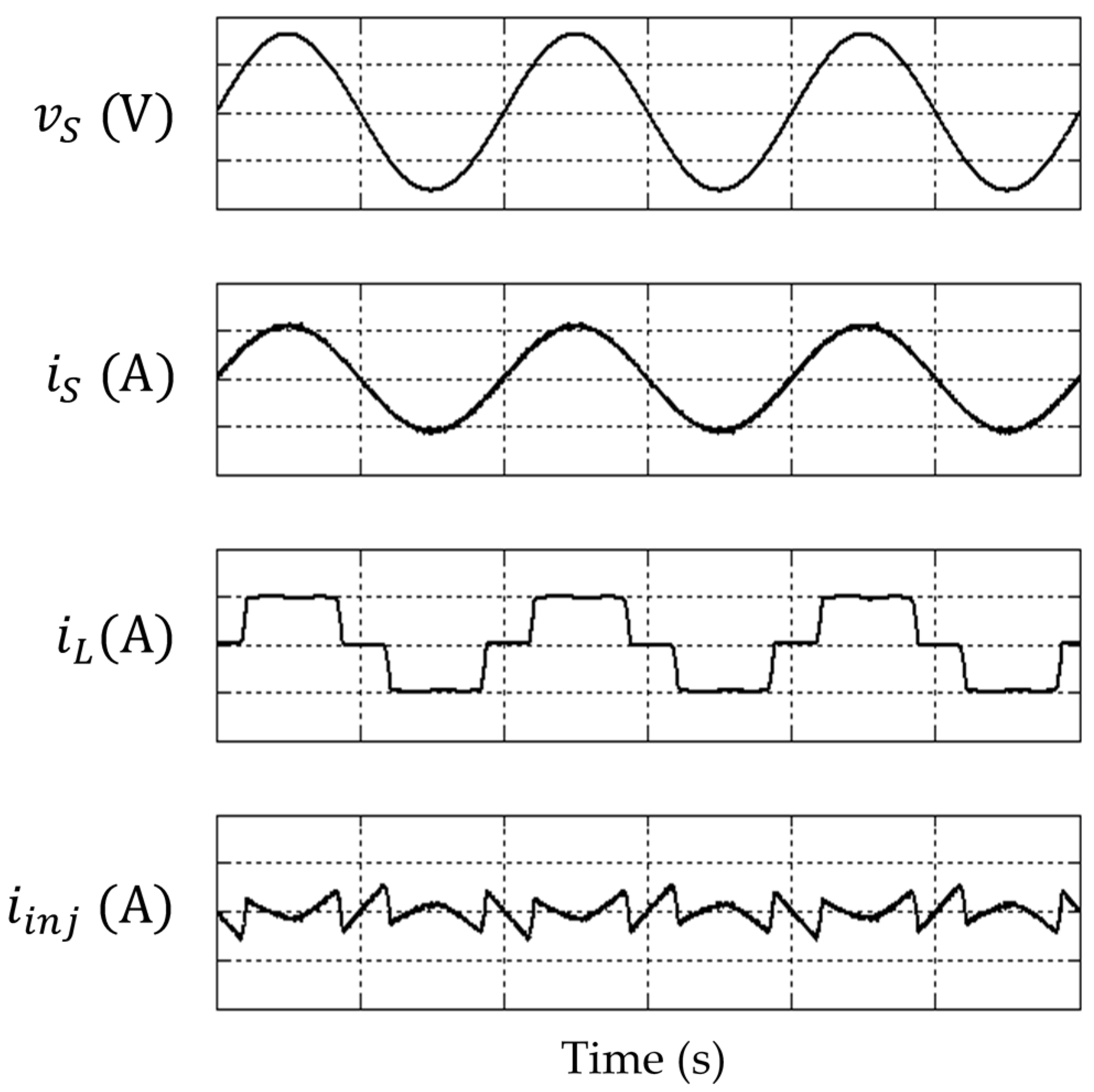

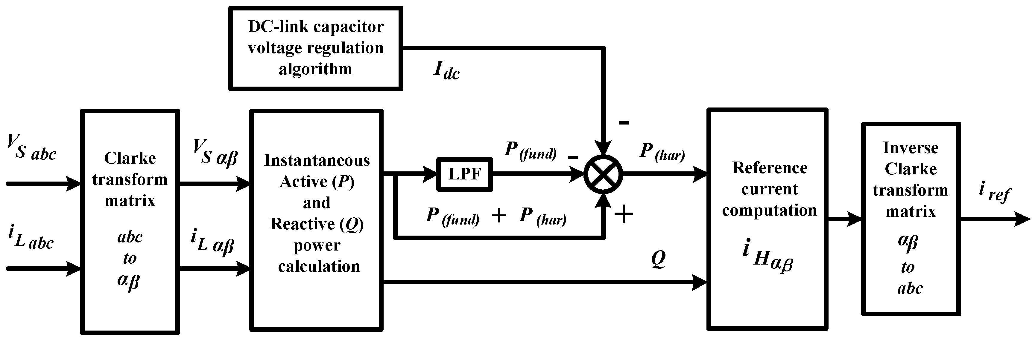

Figure 6.
Control structure of direct voltage error manipulation approach with (a) PI and (b) FLC techniques [38,40].

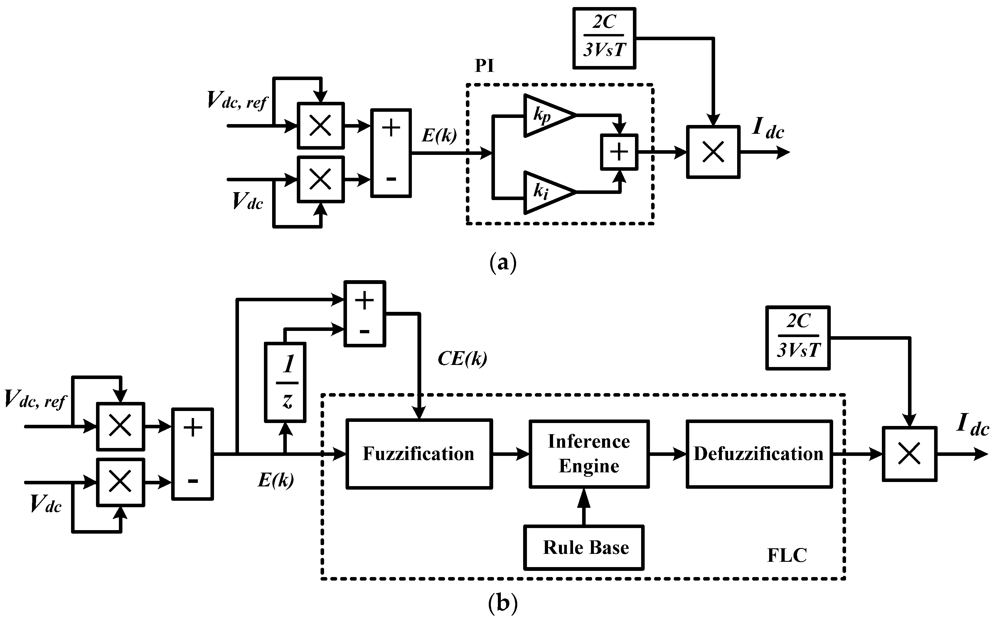
Figure 8.
Conceptual model of direct current control (DCC) scheme.
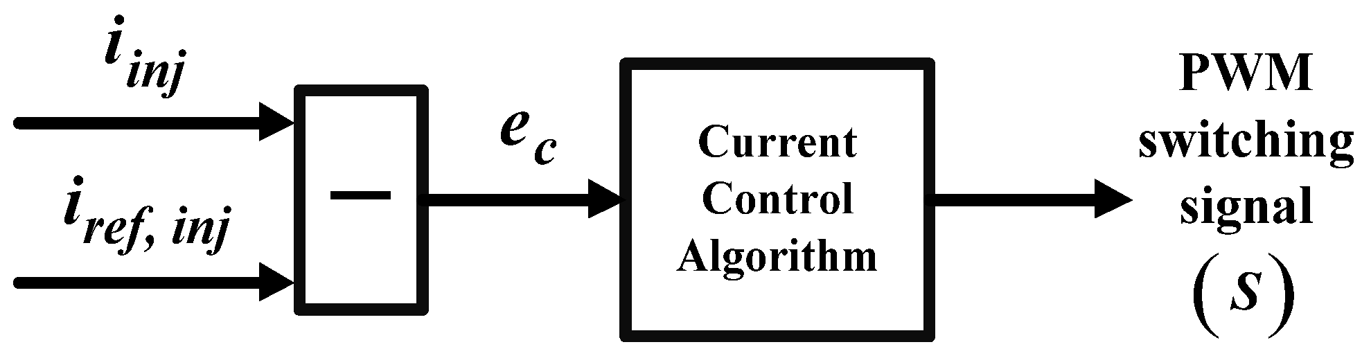
Figure 9.
Conceptual model of an indirect current control (ICC) scheme.

Figure 10.
Conceptual model of a current control scheme with a PWM generator [41].
Figure 10.
Conceptual model of a current control scheme with a PWM generator [41].
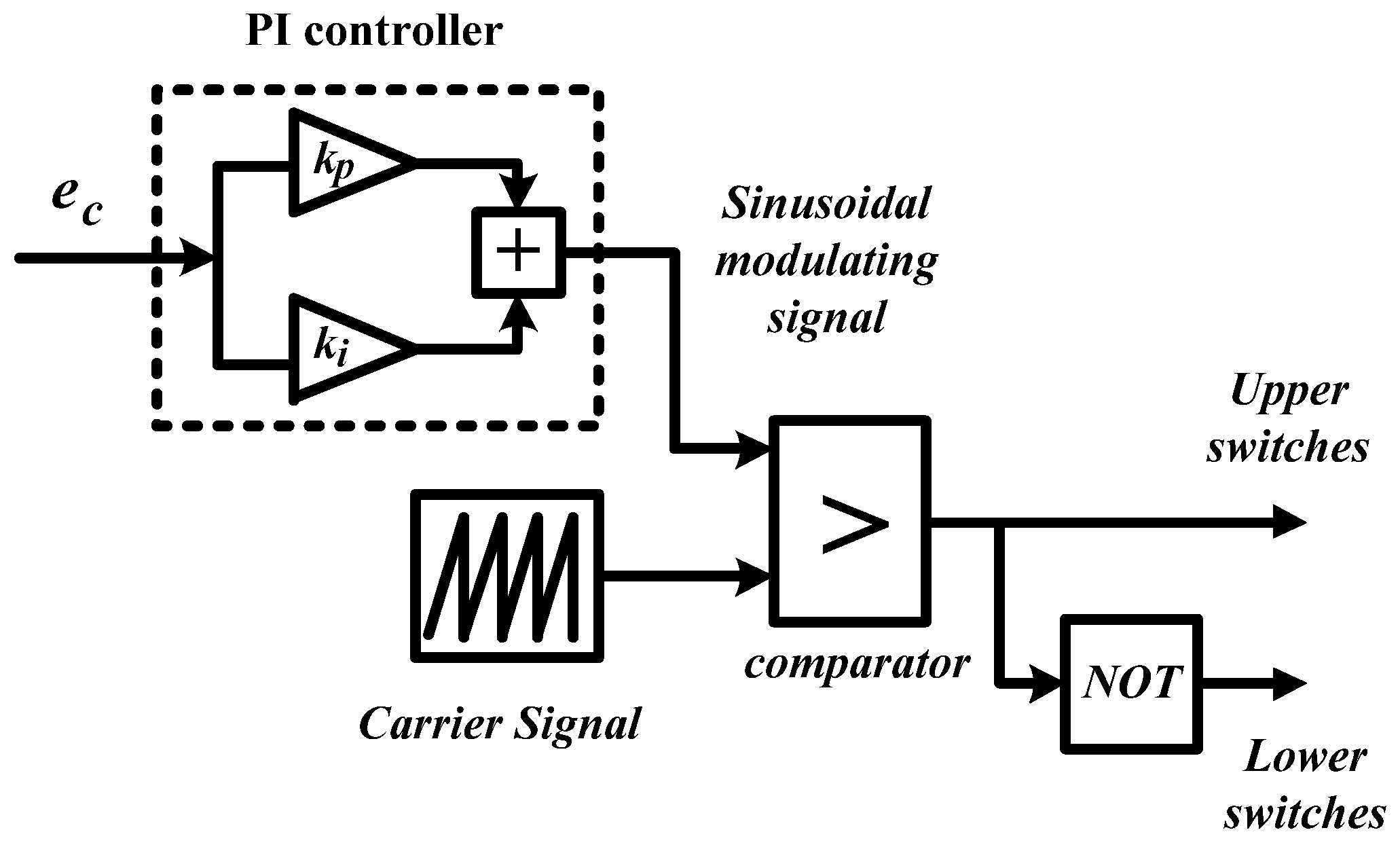
Figure 11.
Conceptual model of a current control scheme based on the space vector modulation (SVM) technique [71,72].

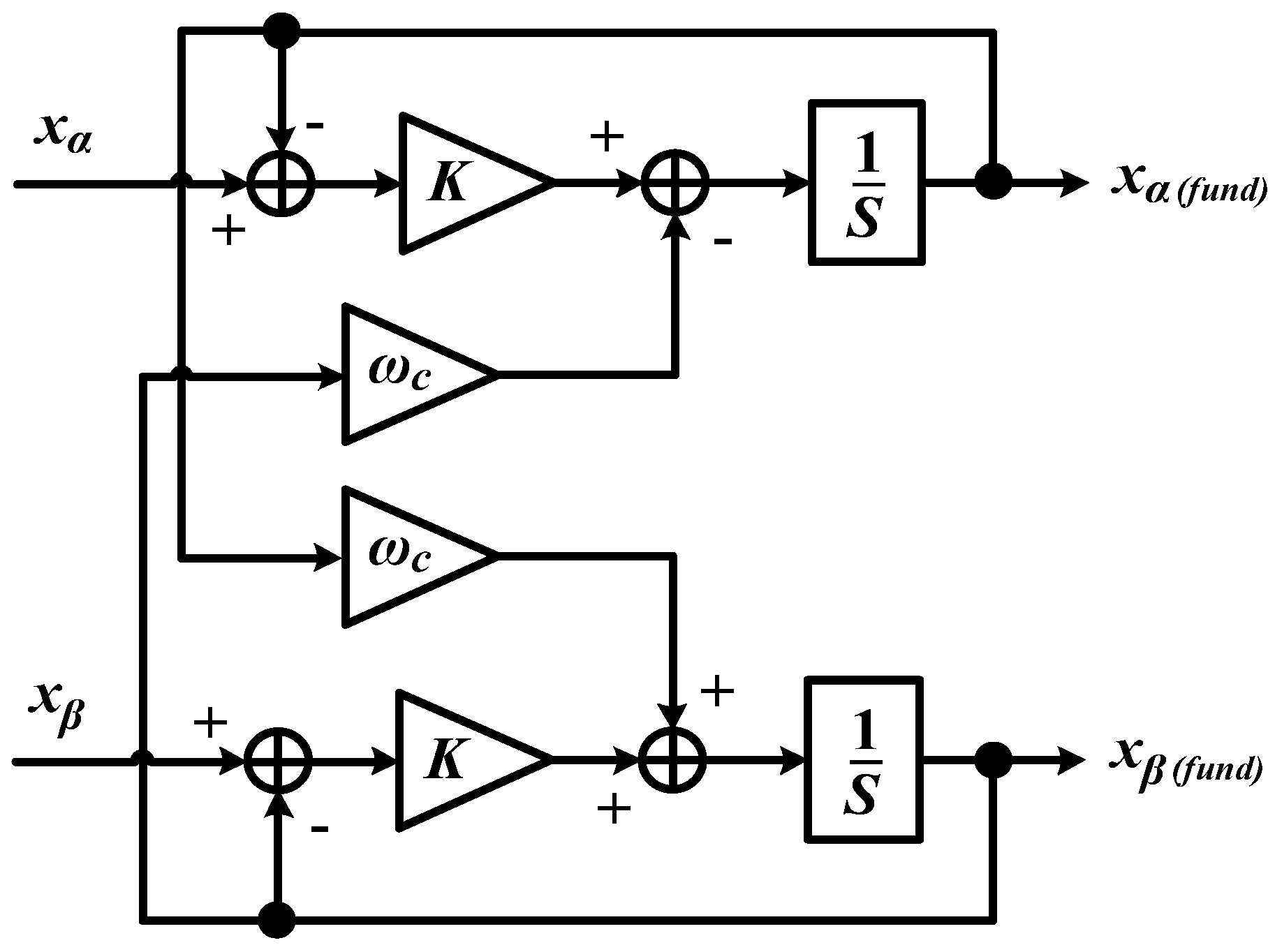
Figure 13.
Theoretical waveforms (phase A) of SAPF’s operation under distorted source voltage conditions.
Figure 13.
Theoretical waveforms (phase A) of SAPF’s operation under distorted source voltage conditions.

Figure 14.
Simplified circuits representation and resulted output voltage waveforms of (a) two-level (b) three-level and (c) n-level inverters [18]
Figure 14.
Simplified circuits representation and resulted output voltage waveforms of (a) two-level (b) three-level and (c) n-level inverters [18]

Figure 15.
Typical circuit topologies of three-phase three-level inverter; (a) CHB (b) NPC and (c) FC [18].
Figure 15.
Typical circuit topologies of three-phase three-level inverter; (a) CHB (b) NPC and (c) FC [18].

Figure 16.
Space vector diagram for three-level NPC inverter; (a) division of sectors and regions, and (b) division of six regions in Sector I for minimizing voltage deviation at neutral-point [69].
Figure 16.
Space vector diagram for three-level NPC inverter; (a) division of sectors and regions, and (b) division of six regions in Sector I for minimizing voltage deviation at neutral-point [69].
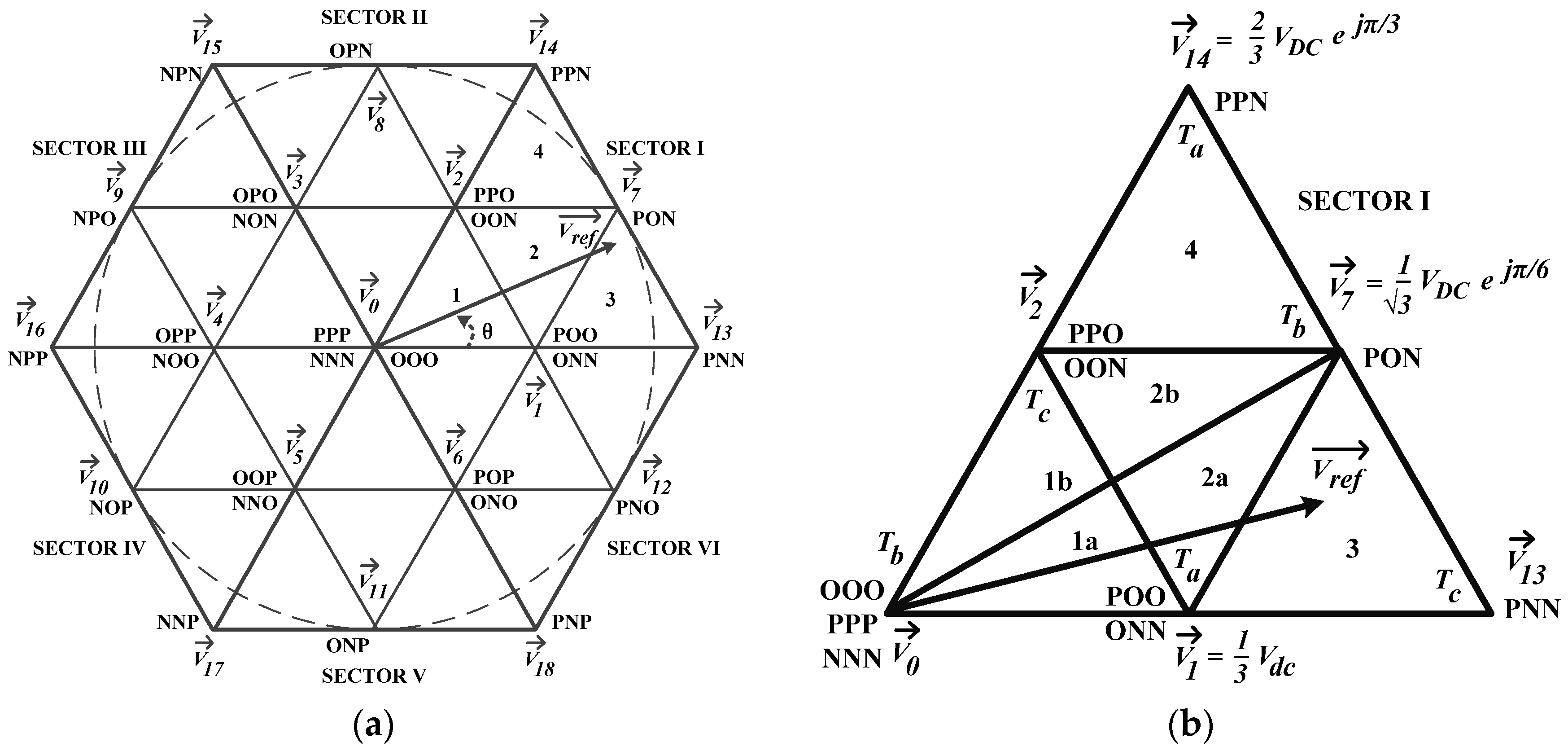

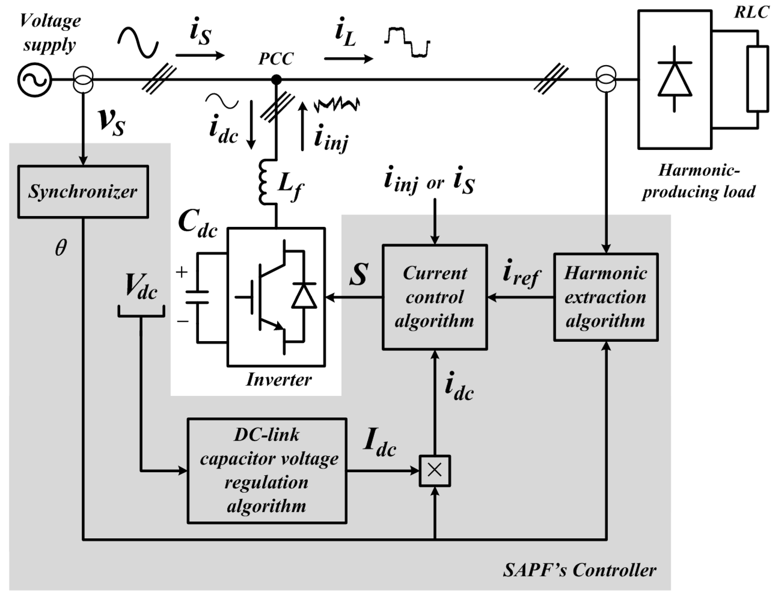
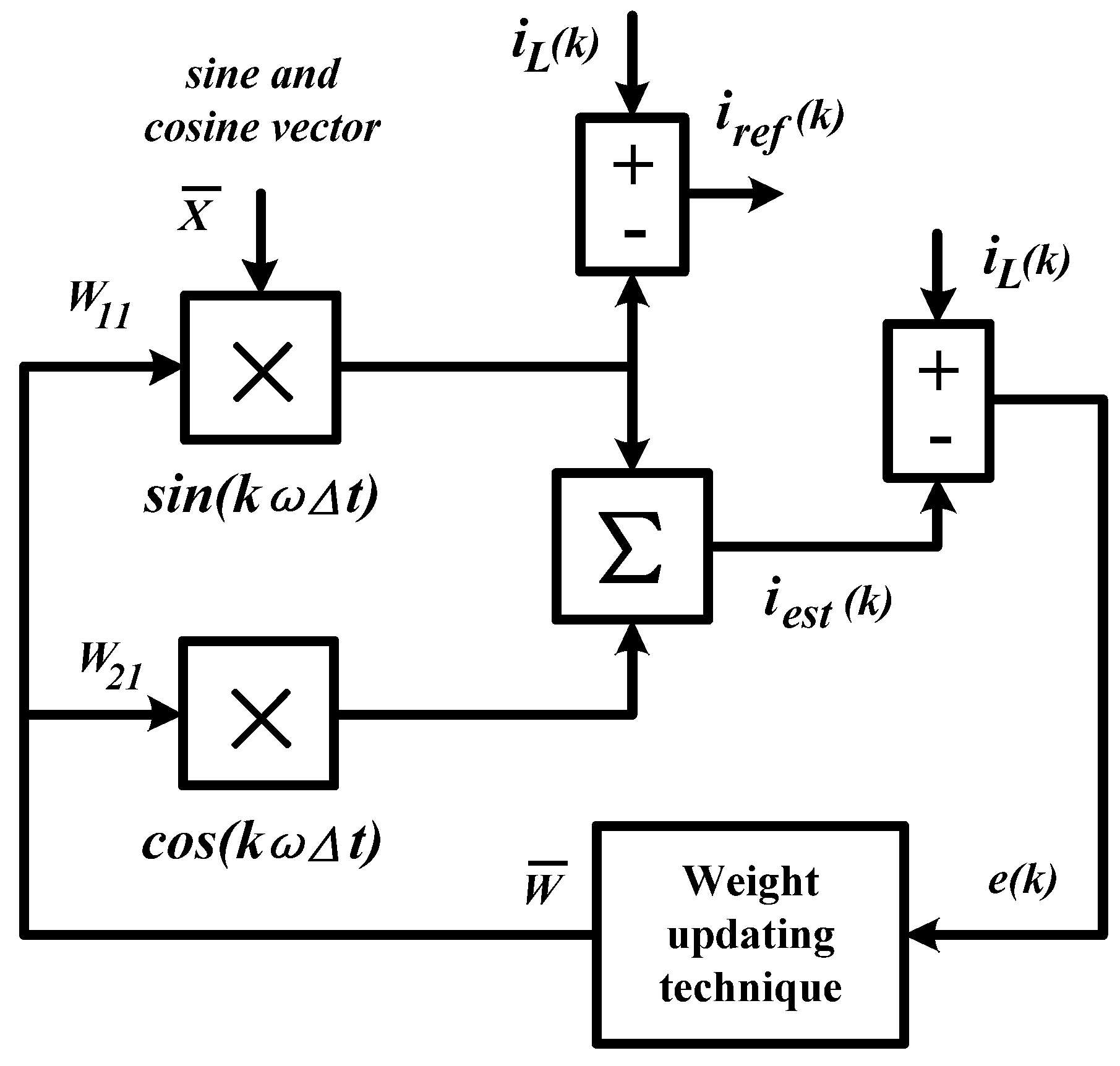
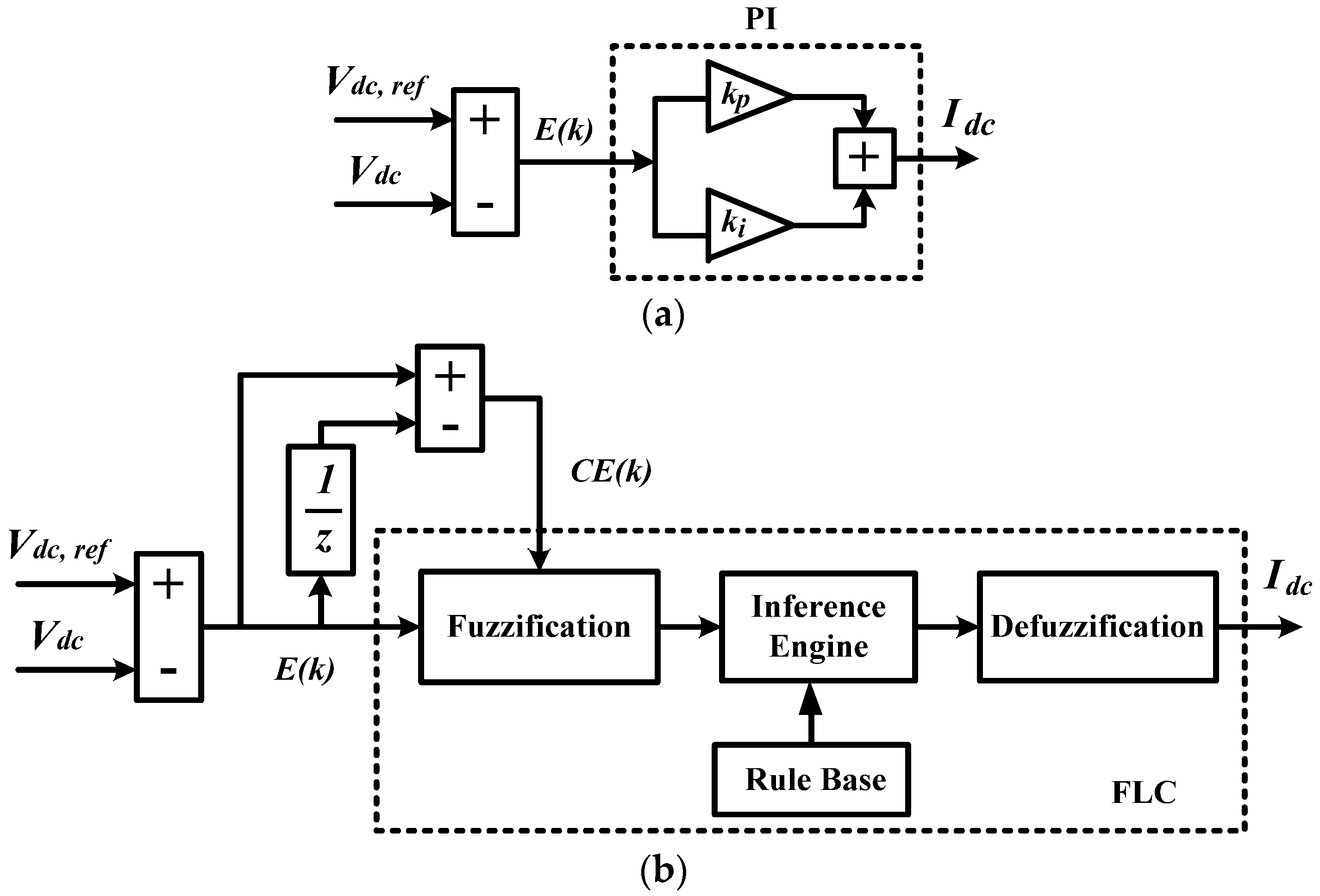
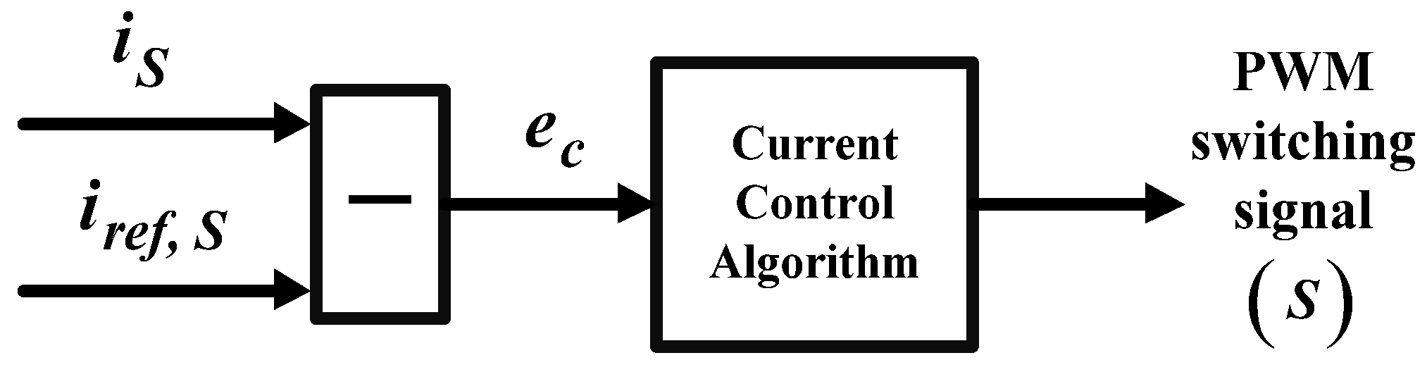
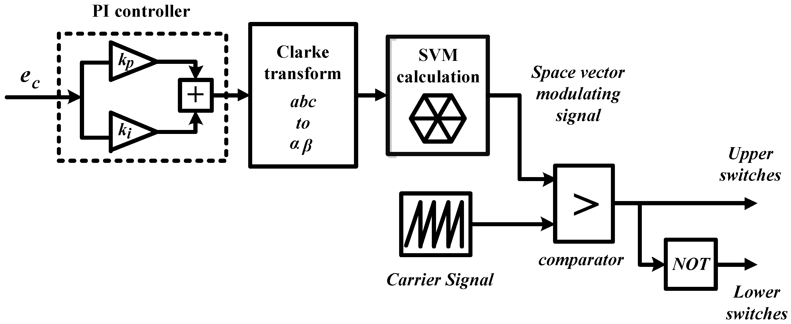
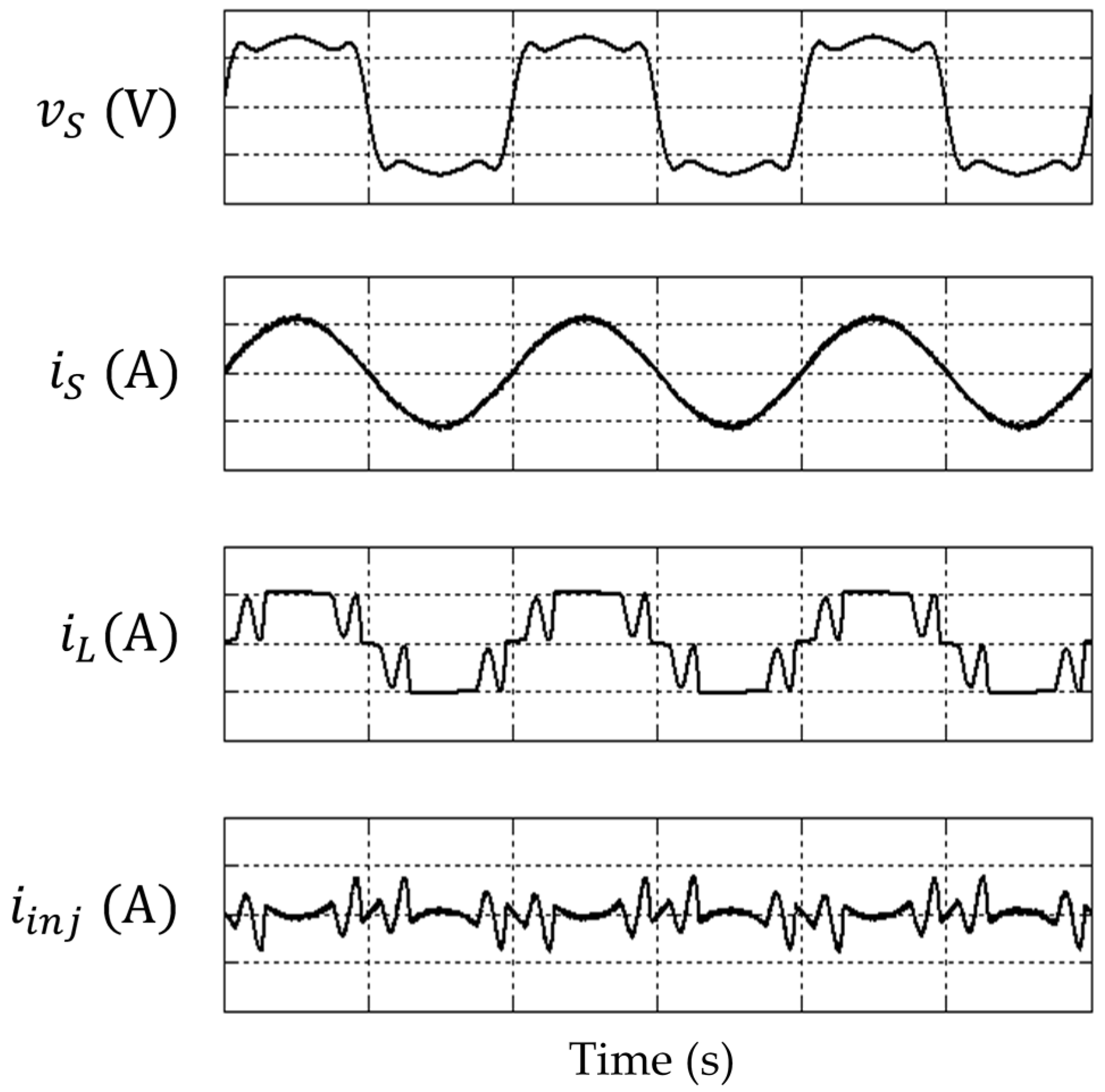
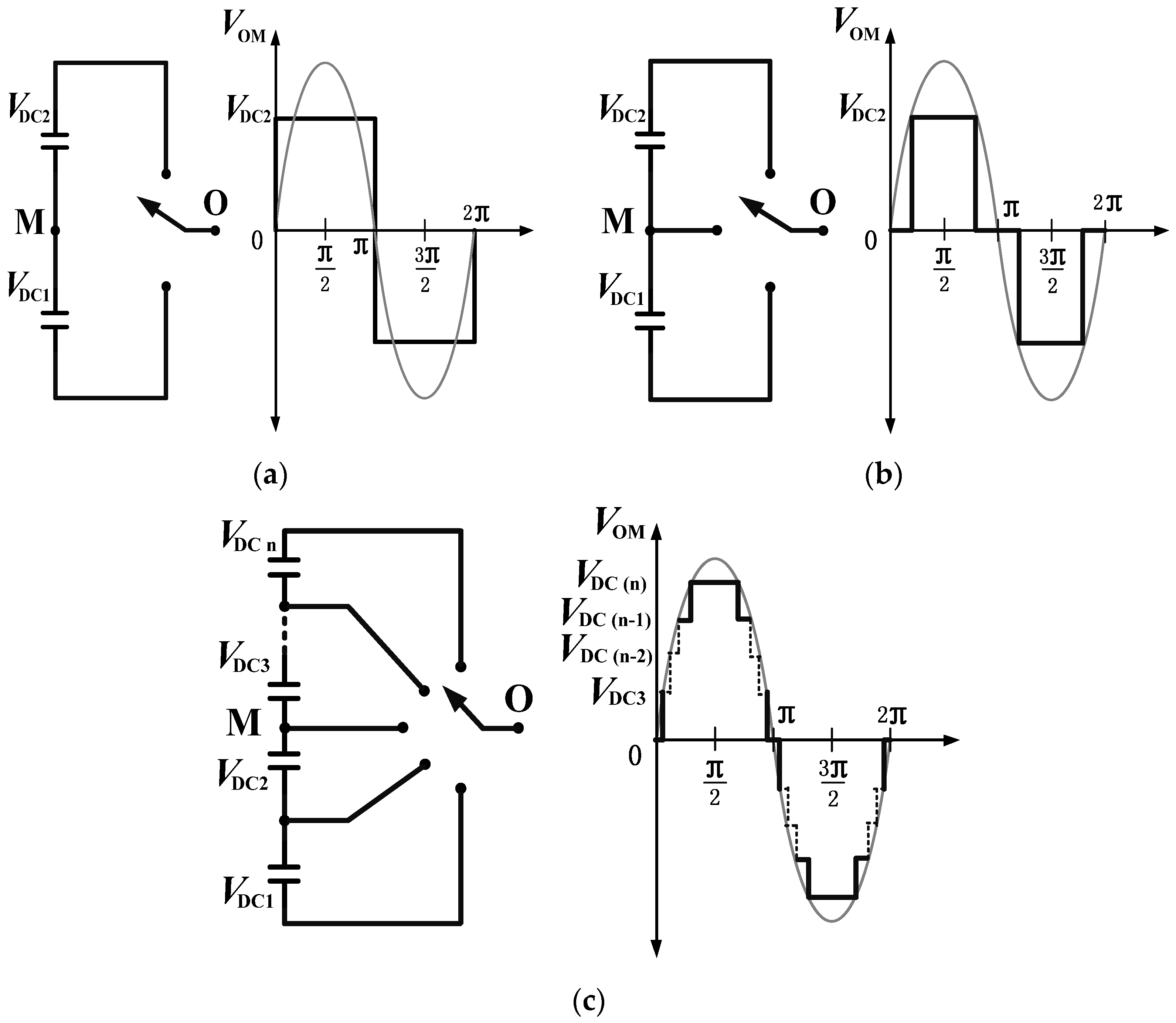
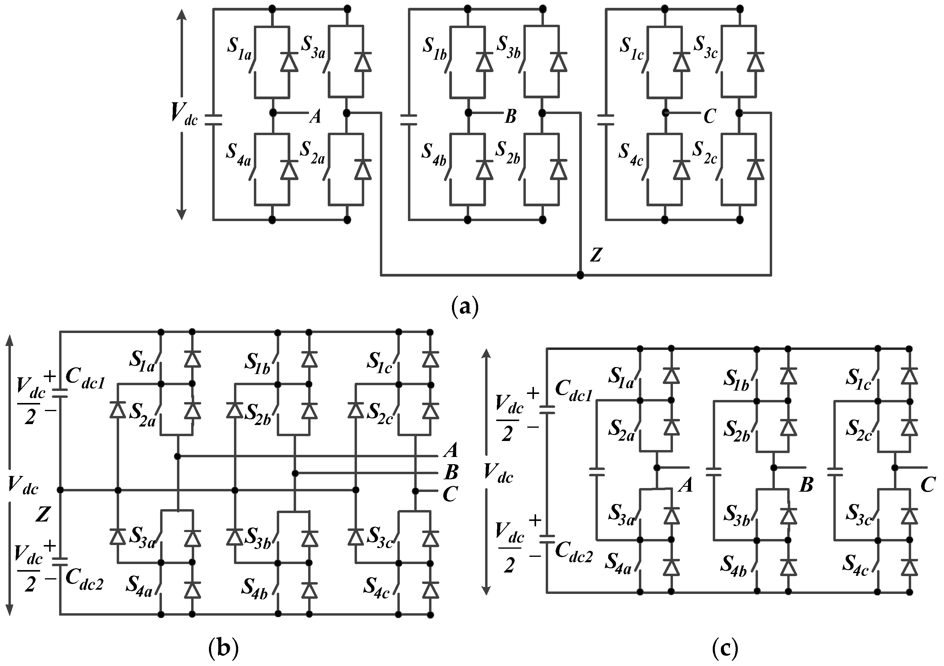
Table 1.
Comparison of multilevel inverter characteristics in three-phase operation.
| Characteristics | Cascaded H-Bridge [102,103] | Neutral-Point Diode Clamped [100,103,104] | Flying Capacitor [18,104,105] | |||||||
|---|---|---|---|---|---|---|---|---|---|---|
| Level | 3 | 5 | n | 3 | 5 | n | 3 | 5 | n | |
| Number of components | Switches with freewheeling diodes | 12 | 24 | 6 (n − 1) | 12 | 24 | 6 (n − 1) | 12 | 24 | 6 (n − 1) |
| DC-link capacitors | 3 | 6 | 3 (n − 1)/2 | 2 | 4 | (n − 1) | 2 | 4 | (n − 1) | |
| Clamping diodes | Not applicable | 6 | 36 | 3 (n − 1)(n − 2) | Not applicable | |||||
| Clamping capacitors | Not applicable | 3 | 18 | 3 (n − 1)(n − 2)/2 | ||||||
| Advantages | Simple structure and control due to its modularity | Robust structure and requires the least amount of DC-link capacitors (less voltage imbalance problems) | Phase redundancy is available to achieve voltage balancing of DC-link capacitors | |||||||
| Limitations | Limited applications due to requirement of separate DC sources | Amount of clamping diodes becomes excessively high with the increase in number of level | Bulky size, high development cost, and complex voltage balancing and switching control algorithm | |||||||
Table 2.
Switching states representation for a three-level NPC inverter [107].
Table 2.
Switching states representation for a three-level NPC inverter [107].
| Switching State | Inverter Switching Status (Phase A) | Terminal Voltage | |||
|---|---|---|---|---|---|
| N | Off | Off | On | On | /2 |
| O | Off | On | On | Off | 0 |
| P | On | On | Off | Off | /2 |
© 2017 by the authors. Licensee MDPI, Basel, Switzerland. This article is an open access article distributed under the terms and conditions of the Creative Commons Attribution (CC BY) license (http://creativecommons.org/licenses/by/4.0/).
Share and Cite
MDPI and ACS Style
Hoon, Y.; Mohd Radzi, M.A.; Hassan, M.K.; Mailah, N.F. Control Algorithms of Shunt Active Power Filter for Harmonics Mitigation: A Review. Energies 2017, 10, 2038. https://doi.org/10.3390/en10122038
AMA Style
Hoon Y, Mohd Radzi MA, Hassan MK, Mailah NF. Control Algorithms of Shunt Active Power Filter for Harmonics Mitigation: A Review. Energies. 2017; 10(12):2038. https://doi.org/10.3390/en10122038
Chicago/Turabian StyleHoon, Yap, Mohd Amran Mohd Radzi, Mohd Khair Hassan, and Nashiren Farzilah Mailah. 2017. "Control Algorithms of Shunt Active Power Filter for Harmonics Mitigation: A Review" Energies 10, no. 12: 2038. https://doi.org/10.3390/en10122038
Note that from the first issue of 2016, this journal uses article numbers instead of page numbers. See further details here.