A Novel Acoustic Liquid Level Determination Method for Coal Seam Gas Wells Based on Autocorrelation Analysis

College of Mechanical and Transportation Engineering, China University of Petroleum-Beijing, Beijing 102200, China
*
Author to whom correspondence should be addressed.
Energies 2017, 10(12), 1961; https://doi.org/10.3390/en10121961
Submission received: 28 September 2017
/
Revised: 14 November 2017
/
Accepted: 21 November 2017
/
Published: 24 November 2017
(This article belongs to the Special Issue Unconventional Natural Gas (UNG) Recoveries 2018)
Abstract
:In coal seam gas (CSG) wells, water is periodically removed from the wellbore in order to keep the bottom-hole flowing pressure at low levels, facilitating the desorption of methane gas from the coal bed. In order to calculate gas flow rate and further optimize well performance, it is necessary to accurately monitor the liquid level in real-time. This paper presents a novel method based on autocorrelation function (ACF) analysis for determining the liquid level in CSG wells under intense noise conditions. The method involves the calculation of the acoustic travel time in the annulus and processing the autocorrelation signal in order to extract the weak echo under high background noise. In contrast to previous works, the non-linear dependence of the acoustic velocity on temperature and pressure is taken into account. To locate the liquid level of a coal seam gas well the travel time is computed iteratively with the non-linear velocity model. Afterwards, the proposed method is validated using experimental laboratory investigations that have been developed for liquid level detection under two scenarios, representing the combination of low pressure, weak signal, and intense noise generated by gas flowing and leakage. By adopting an evaluation indicator called Crest Factor, the results have shown the superiority of the ACF-based method compared to Fourier filtering (FFT). In the two scenarios, the maximal measurement error from the proposed method was 0.34% and 0.50%, respectively. The latent periodic characteristic of the reflected signal can be extracted by the ACF-based method even when the noise is larger than 1.42 Pa, which is impossible for FFT-based de-noising. A case study focused on a specific CSG well is presented to illustrate the feasibility of the proposed approach, and also to demonstrate that signal processing with autocorrelation analysis can improve the sensitivity of the detection system.
1. Introduction
Mine gas is one of the most serious safety hazards in coal mining [1]. It is reported that 19 gas accidents with 100 fatalities or more have occurred in Chinese coal mines from 1950 to 2012 [2]. The exploitation of coal seam gas (CSG) would reduce the incidence of coal-gas outbursts, as CSG pre-drainage can reduce the gas content and pressure in coal [3]. In addition, it is clear that the CSG is a significant source of energy. Nowadays, growing attention is being paid to CSG recovery, particularly in China [4]. CSG is produced by lowering the pressure within the coal seam so that methane is released from the coal in the form of gas and then brought to the surface accompanied by the water [5]. CSG production is closely related to water drainage which is a prerequisites for reducing the reservoir pressure and desorption of adsorbed gas [6,7]. However, improper water and gas production at the initial stage may result in permeability damage and further induce the change in productivity [8]. Even worse, too fast a dewatering rate can lead to an unfavorable ultimate recovery [9]. The water depth plays an important role in gas production associated with CSG recovery and adjustment of production parameters to ensure CSG wells in the best conditions [10,11]. Therefore, it is of great significance to accurately monitor the liquid level in order to calculate gas flow rate and well performance for optimizing gas production of CSG wells.
The commonly used method for annular liquid level measurement is the acoustic liquid level test [12,13]. It determines the depth of liquid level by counting the acoustic waves reflected from tubing collars or velocity-time products [14]. The advantages of this acoustic analysis include an inexpensive and non-intrusive process resulting in its wide applications across the world, compared to mechanical, capacitive and optical methods [15,16]. In a production gas/oil well, the gas/oil flows in the tubing and annular partial obstructions, poor surface connections or odd length of tubing joints are the main disturbing factors for annulus liquid level measurements [17]. By enhancing the sensitivity of acoustic sensors, adopting downhole markers as references for acoustic propagation distance and acquiring with high and low frequency data from dual channels, the liquid level can been located under these unusual conditions [18,19]. However, the improvement of the measurement accuracy by enhancing the sensitivity of the acoustic sensors is limited due to the inherent performance characteristics of the sensors. In addition, downhole conditions will impact the effectiveness of acoustic speed correction from downhole markers. What’s more, there is still no effective filtering method to tackle the effect of noise with a similar frequency as the signal.
In a CSG well, once critical desorption pressure is achieved, mine gas will be desorbed from the matrix and flow upward in the annulus, which causes new problems such as violent degassing, foaming and noise from the high gas rate for annular liquid level determination [20]. For the violent degassing and foaming condition, McCoy et al have introduced a mathematical formulae method of foam-free liquid level determination based on surface acoustic liquid level by measuring data acquired within the narrow time window available for closing the casing valves [21]. The study of Bhargava et al has proved that this method has easy, simple and cost effective advantages avoiding downhole intervention. Nevertheless, the existing problem of shutting in the well restrict its broader application, for example, a real-time test is impossible [22]. Han developed an automatic echosounder system which can acquire acoustic signals under intense gas interference. High noise-to-signal data is filtered using a spectral decomposition-based digital filtering algorithm as a key technology to realize the gas/liquid level detection under aerated liquid column conditions [23]. In general, the measurement error of 1.00% of the system is still large for industry practices [24,25]. In particular the low frequency noise cannot be removed by using a spectral decomposition-based digital filtering algorithm, as the frequency of the noise is similar to the acoustic signal. A better understanding and improved solution to the specific problem of low frequency noise cancellation from acoustic echo signals is thus needed to effectively reduce the interference in identifying the acoustic signal reflected by the liquid level for CSG wells.
Normally, the liquid level is located by the distance that equals half the product of the acoustic velocity and the travel time in the annulus [26]. It is widely known that the temperature and the pressure change with the depth of the well, which will have an impact on the annular acoustic velocity. In 1962, Ramey first developed an approximate solution to calculate the temperature in an injection well [27]. Then Hasan and Kabir improved Ramey’s model by allowing for two-phase flow and using a new transient solution of overall heat transfer coefficient [28]. With consideration of the temperature effect, the annular pressure varies with the depth [29,30]. It is demonstrated that the production rate has a main influence on the pressure behavior of the annulus in a certain well [31]. In addition, the propagation velocity of sound wave has nonlinear relation with the temperature and the pressure of the media [32]. Therefore, this speed variation can lead to a large error in liquid level determination, if it is regarded as a linear model.
In order to overcome these abovementioned limitations, the objective of this paper was to develop a new method based on ACF for the annulus liquid level determination in CSG wells. This method involves the calculation of the acoustic travel time in the annulus and processing the autocorrelation signal in order to extract the weak echo under the intense noise interference. The random errors can be reduced by calculating the acoustic propagation time from the overall correlation of the initial pulse and reflected one. The non-linear dependence of the acoustic velocity on temperature and pressure is taken into account. In addition, the experimental laboratory investigations are developed for liquid level detection, integrating with low pressure, weak signal, and intense noise generated by gas flowing and leakage. At last, an evaluation indicator called Crest Factor and measurement error is adopted to validate the superiority of the ACF-based method compared to Fourier filtering (FFT).
The rest of this paper is organized as follows: Section 2 presents the principle of acoustic liquid level determination. In Section 3, a novel method is developed for determining the acoustic liquid level of CSG wells based on autocorrelation analysis paying more attention to noise jamming. In Section 4, laboratory experimental investigations are conducted for liquid level testing under conditions with the different annulus pressures and noise levels resulting from leakage. A case study focusing on a CSG well is introduced in Section 5 to demonstrate the application of the proposed models. Concluding remarks are given in Section 6.
2. Principles of Acoustic Liquid Level Determination
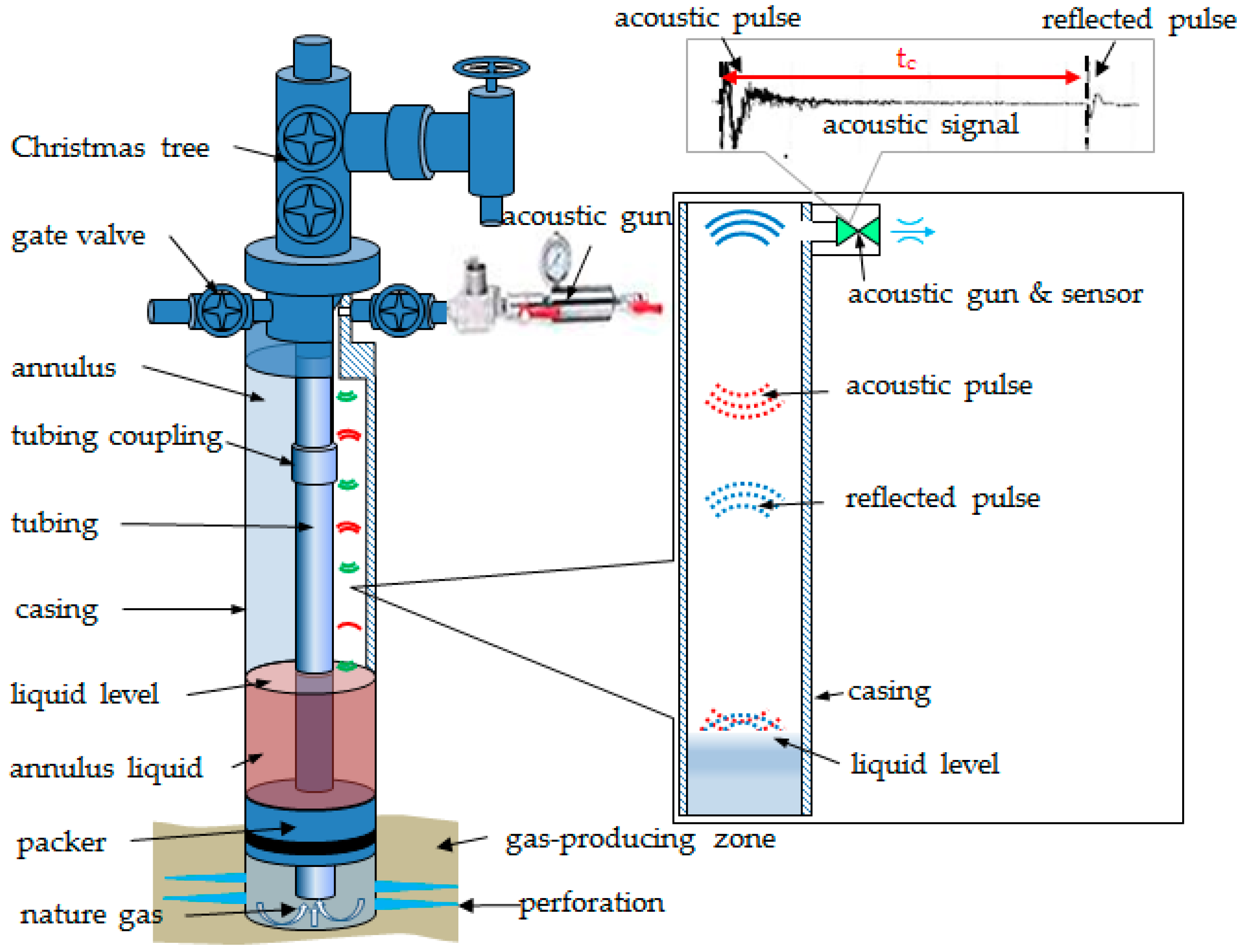
The principle of acoustic liquid level determination is shown in Figure 1, where an acoustic gun attached to the wellhead of the annulus is used to emit an acoustic pulse, and then the acoustic pulse spreads across the annulus from surface to bottom. When the acoustic wave encounters restrictions, such as tubing coupling and subsurface safety value, a partial acoustic wave will be reflected to the wellhead and received by the acoustic sensor. Specially, as soon as the acoustic wave reaches the liquid level, all the wave will be completely reflected by the interface, and the acoustic sensor will receive a reflected wave of high intensity later. By identifying the reflected signal from the liquid level, the round-trip (surface-liquid level-surface) travel time of the acoustic wave can be determined. And then the depth of the liquid level zt will be obtained from the following equation [33]:
where t and W are the round-trip travel time and the propagation velocity of the acoustic wave in the annulus, respectively.
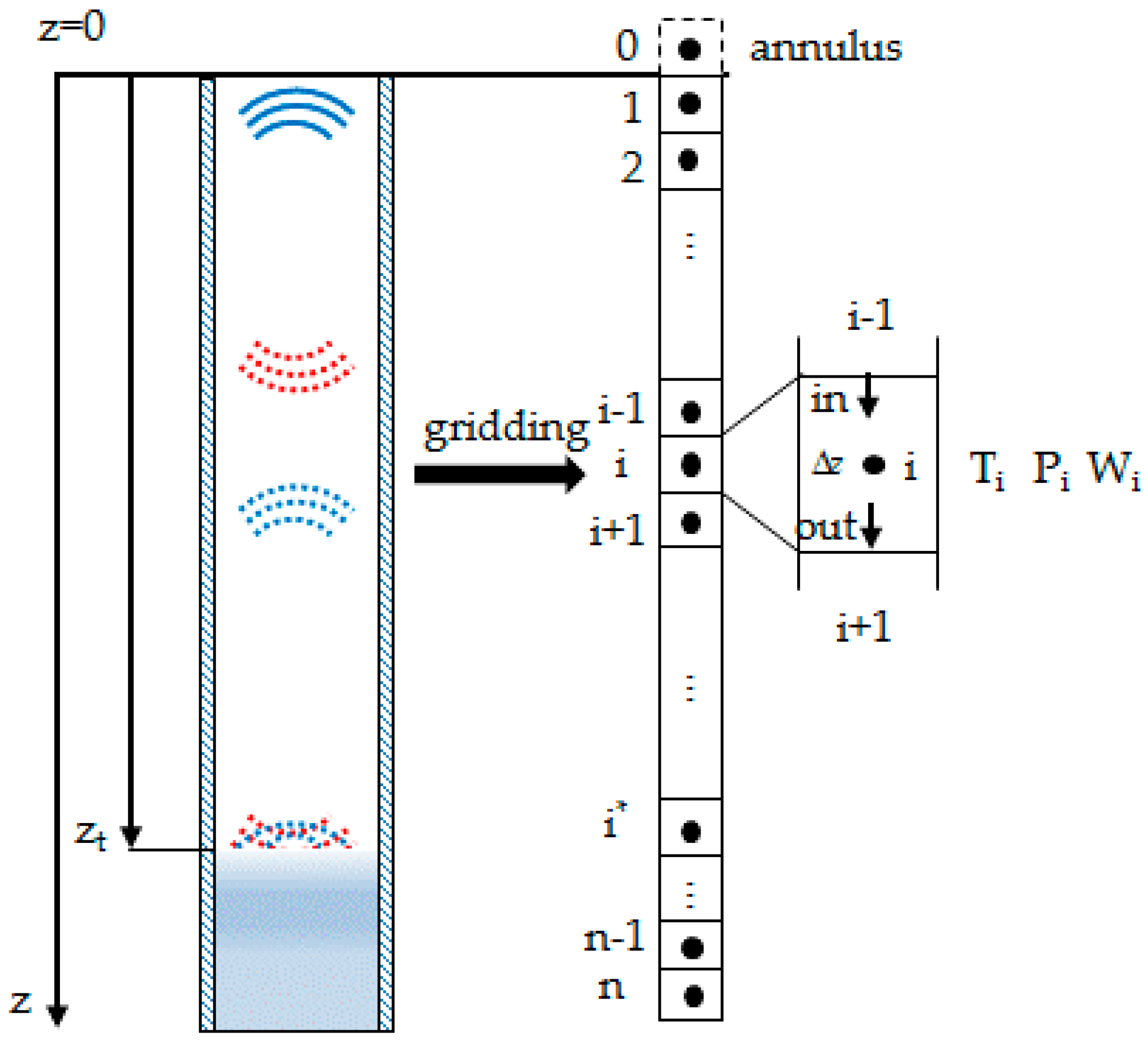
The halfway of the acoustic propagation in the annulus will be considered for simplicity due to symmetry. Obviously, the pressure and the temperature of annulus will change along the depth, leading to variation in the velocity of the acoustic propagate in annulus. The calculation of Equation (1) is intractable to acquire and an iterative method is therefore developed to calculate the depth of the liquid level using the computational mesh as shown in Figure 2. It is divided into n grids for the computational domain within the annulus. If the length Δz of the cell is short enough, the pressure, the temperature and the velocity of acoustic propagate within the cell can be considered as constant variables. Therefore, the new acoustic travel time to cell i* can be determined by:
If is extremely close to the actual measured halfway travel time of the acoustic pulse propagation in the annulus, cell i* is considered as the position of the liquid level. Besides, the distance of acoustic pulse propagation from wellhead to cell i* is equal to the depth of the liquid level. The term zt can be expressed as:
The process of calculation is greatly simplified by the iterative algorithm and it is critical for accurately determining the depth of the liquid level to obtain the travel time and the propagation velocity of acoustic pulses in the annulus. The details of acquiring the actual test travel time of the acoustic pulse and computing the velocity of acoustic propagate in the annulus are expounded in the next section.
3. Development of an Acoustic Liquid Level Determination Method
The new method used for acoustic liquid level determination is described in this section. This method includes models that are highlighted for firstly calculating acoustic velocity and acoustic travel time in annulus, and then determining the acoustic liquid level of a gas well.
3.1. Acoustic Velocity in Annulus
The acoustic velocity in annulus is mainly related to the composition, temperature and pressure of the annulus. It can be derived from energy balance around a stationary wave undergoing an infinitesimal perturbation [34,35]:
where Cυ, Cp and z is the heat capacity at the constant pressure, J/(kg·K), the heat capacity at the constant volume, J/(kg·K) and the compressional factor, respectively. All three parameters can be calculated by using the equations demonstrated by Aly and Lee [36]. Mr is the molar mass of gas mixtures, which is presented as:
where xi is the mole fraction of component i of the natural gas in annulus. Mri is the molar mass of component i of the natural gas. N is the number of the components in the natural gas. According to the research of Ahmadi, Cυ, Cp and z are a function of the temperature and pressure of the gas with certain components [37]. The distribution of the temperature and pressure in the casing annulus of a gas well is therefore determined before the calculation of acoustic velocity.
3.1.1. Modeling of Annulus Temperature
In order to establish the model for calculating the temperature of the annulus, an infinitesimal length () of a well is taken for analysis, as shown in Figure 3. It is assumed that the flow in the tubing is in one-dimensional steady state, and the heat exchanges only occur in the radial direction between the wellbore and the surrounding formation, regardless of the heat transfer in the vertical direction. The tubing and casing are also supposed to be concentric.
According to the energy conservation principle, the temperature gradient of the fluid in the tubing can be expressed as [38]:
where Tf is the fluid temperature, K. z is the vertical depth, m. g is the gravitational acceleration, m/s2. υ is the flow velocity of natural gas, m/s. Cpm is the mean heat capacity of the wellbore fluid, J/(kg·K). P is the pressure, Pa. CJ is the Joule Thomson coefficient, J/(kg·K). Q is the heat exchange capacity per unit mass, J/kg.
Based on the principle of energy conservation, the heat transfer from the fluid to the cement Q1 is equal to that from the cement to the formation Q2:
where Tcem is the cement temperature, K. Th is the formation temperature which increases linearly with the depth of formation, K [39]. TD is the time function of transient heat transfer which can be described by the approximate formula recommended by Hasan and Kabir [28]. U0 denotes the overall heat transfer coefficient, which is defined as [26]:
where Rti, Rto, Rci, Rco and Rcm represent the inner diameter of tubing, outside diameter of tubing, inner diameter of casing, outside diameter of casing and outside diameter of cement sheath, respectively, (m) and hf, ki, hc, hr, kcas and kcem represent the convective heat transfer coefficient of fluid in tubing, the thermal conductivity of tubing, the convective heat transfer coefficient of fluid in annulus, the radiation heat transfer coefficient of fluid in annulus, the thermal conductivities of casing and cement respectively (W/m2·K), as shown in Figure 3. In general, the overall heat transfer coefficient is certain for an identified well.
Sagar introduced the term φ to combine the Joule-Thomson and kinetic-energy terms into a single term [40]. According to Equations (4) and (5), the temperature distribution of the fluid in tubing can be acquired:
where:
The heat transfer from annulus to cement can be described as:
As the heat transfers from annulus to cement is equal to that from the cement to the formation [41], the annulus temperature Tc at a certain depth can be expressed by combining Equations (7) and (11):
3.1.2. Modeling of Annulus Pressure
Another important parameter for determining the acoustic velocity is the annular pressure. The annular pressure distribution of the gas in the sealed annulus can be calculated on the basis of the energy equation:
where ρg is the annular gas density (kg/m3). The gas density can be derived from the following equation, according to the gas state equation [42]:
By integrating Equation (13) from the bottom to the top of the well segment of depth Δz, the annulus pressure in production casing can be calculated as follows:
where Pc_out and Pc_in represent the outlet and inlet pressure of the segment, respectively. In short, the acoustic velocity can be calculated when the pressure versus depth and temperature profile are known. Then, the acoustic travel time in the annulus is needed to determine the liquid level.
3.2. Acoustic Travel Time in Annulus
3.2.1. Characteristics Analysis of Test Acoustic Signal
An acoustic sensor is installed in the gas gun shown in Figure 1 to test the signal consisting of the initial acoustic pulse and reflections from liquid level. The acoustic travel time in the annulus can be obtained by computing the interval from initiating the acoustic pulse to receiving the pulse reflected. The time domain and the frequency domain of acoustic signal of a typical gas well are presented in Figure 4. The frequency of the acoustic signal is mainly concentrated in the area beyond the frequency of 20 Hz, namely, its energy is focused on the low frequency. This is because the high frequency portions of the signal are absorbed by the medium in the annulus during propagation.
As indicated in Figure 4a, reflections of the liquid level are periodically measured because the pulse will bounce back and forth both from the wellhead and the interface of the annulus liquid. For periodic signals containing random noises, the noise component can be eliminated by autocorrelation processing effectively, which is the greatest advantage of autocorrelation analysis compared to other noise-reduction methods. Therefore, autocorrelation analysis algorithm is adopted to reduce the noise and to identify the cycle of useful signals (acoustic reflections) under high noise condition.
3.2.2. Principles of Autocorrelation Analysis for Test Acoustic Signal
The autocorrelation function (ACF) of the continuous signal x(t) is defined as [43]:
where, τ denotes the delay time.
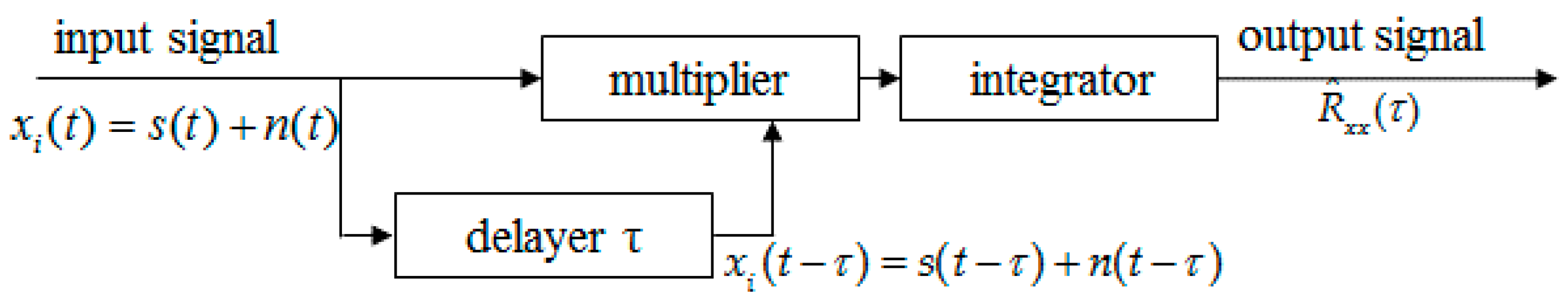
Figure 5 shows the principle of autocorrelation analysis. Assuming that a signal xi(t) is the useful signal s(t) mixed with the noise n(t), then the signal xi(t) can be expressed as
The delay function xi(t − τ) can be obtained based on signal xi(t) delayed by time τ.
We transmit the delayed signal xi(t − τ) and the original signal xi(t) to the multiplexer. The is obtained by taking the integral of xi(t − τ)·xi(t) and then giving an average of it. Based on the abovementioned, the final ACF with the variable τ can be obtained as Equation (19):
where and denote the cross correlation function of the signal and noise, respectively. and are both zero, because the noise and the signal are usually uncorrelated. is the ACF of the noise signal itself. As the time delay increases, approaches zero. As a result, the output of the ACF is only . The noise is therefore effectively suppressed and the desired signal is identified.
3.2.3. Estimation for ACF of Test Acoustic Signal
The collected acoustic signal is converted to the digital signal and then transmitted to a computer. Corresponding to the digital acoustic signal x(n), its ACF is presented as [44]:
In general cases, we can estimate the ACF by utilizing the method below. If n > N, we can obtain N measured values of x(n). Based on the measured values, is calculated as:
Generally, the ACF is expressed in a normalized form which has a scale of ±1, namely the correlation coefficient ρss(τ) defined as [45]:
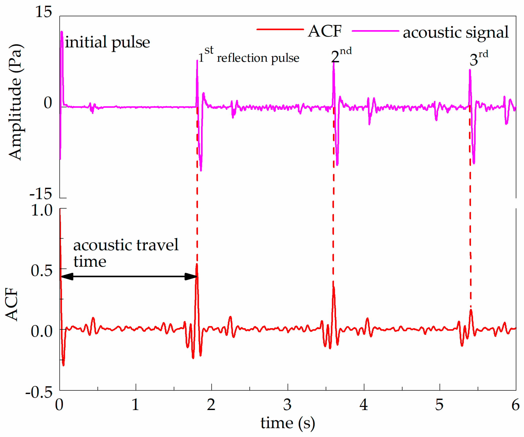
Figure 6 shows the ACF of the acoustic signal in Figure 4a. As indicated in Figure 6, the acoustic sensor receives the reflected pulse three times during the sampling time. Normally, the computer software locates the liquid level by extracting the peak of the reflected pulse, while for the ACF method, the acoustic propagation time within the annulus is calculated from the overall correlation of the initial pulse and reflected pulse, which can avoid the random errors. In addition, the autocorrelation analysis of the acoustic signal can remove the low frequency noise that the traditional spectrum analysis method cannot do. Therefore, the obvious contribution of this algorithm is that it can greatly improve the test accuracy and ability of liquid level determination.
3.3. Determination of Acoustic Liquid Level
The pressure and temperature of the annulus at the wellhead and acoustic signals are measured by the liquid level detection system. Then an iterative model is developed to calculate the pressure, temperature and velocity along the annulus using computational mesh shown in Figure 2. The velocity is stored in cell centers of control volumes, whereas the scalar variables of the annular pressure and temperature are located at cell faces. Then the acoustic velocity and travel time in every cell can be calculated. By comparing the computed acoustic travel time and real results, the pulse transmitting distance is obtained until their difference is less than the given error. It’s important to note that the real tested acoustic travel time is the round-trip travel time. It should be divided by 2 to calculate the depth of the liquid level which is only half the propagation distance of sound. The detailed steps of the iterative procedure for locating the liquid level are explicitly illustrated as follows, and the overall workflow is shown in Figure 7.
- Divide the well into n cells with the same length Δz in the depth direction;
- The pressure and temperature of the first cell are equal to that measured at the wellhead;
- For the cell i, a value of annulus pressure is assumed.
- Calculate the annulus temperature ;
- Calculate the annulus pressure Pci;
- Check if . If so, go to next cell. If not, assume a new value of annulus pressure and go back to step 2.
- Calculate the acoustic velocity Wci;
- Calculate the acoustic travel-time ;
- Calculate the cumulative travel time from surface to current depth ;
- Repeat step 3 to step 9, until ;
- The depth of the liquid level is equal to zi = i*Δz.
4. Acoustic Liquid Level Detection Experiments
In order to reveal the advantages of the proposed method in extraction ability and measurement accuracy, an experimental setup for liquid level tests has been established, and a comparative study between the ACF-based and FFT-based denoising methods has been carried out under different sound pressures and noise levels.
4.1. Discriptions of the Experimental Devices
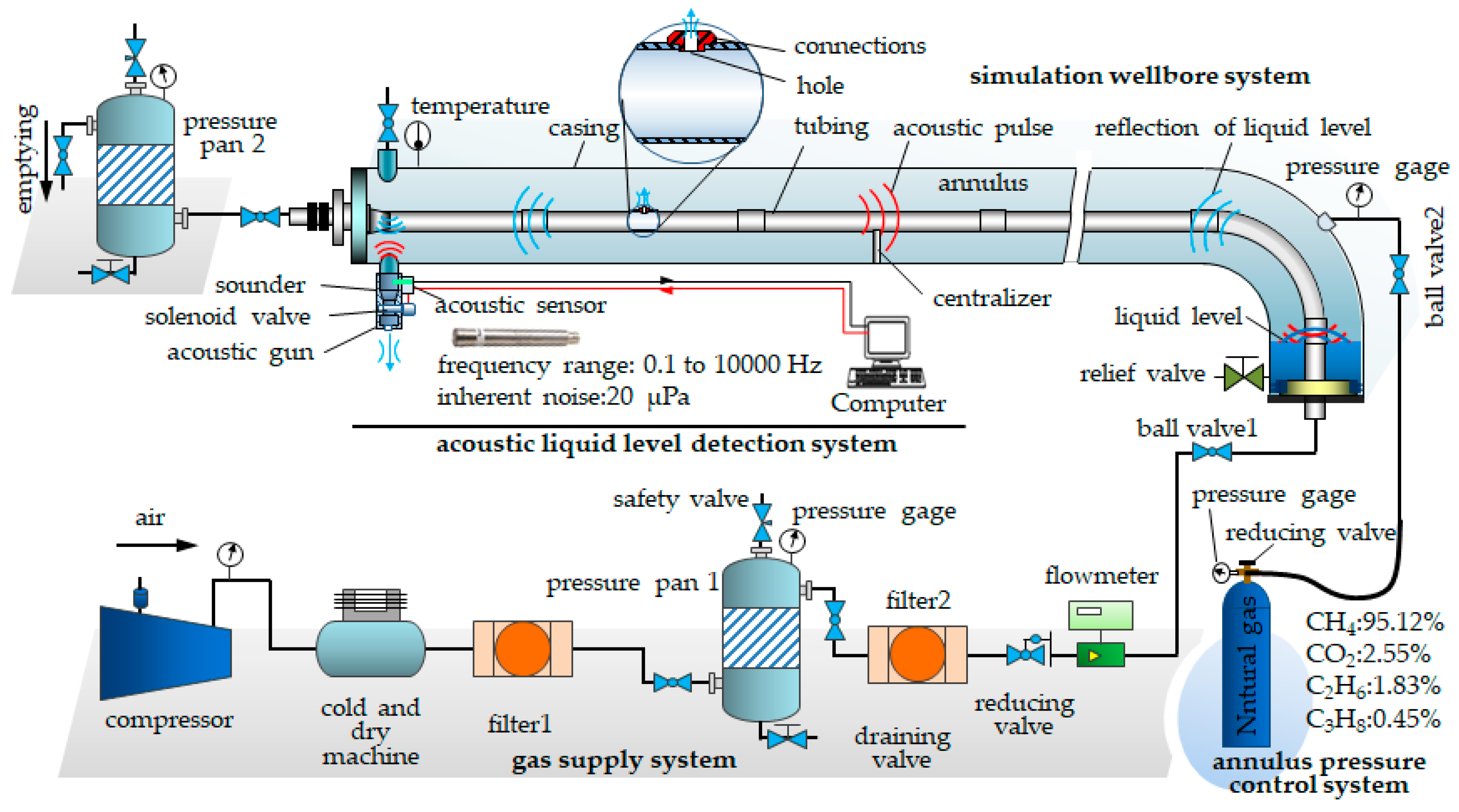
The main functions of the experimental setup are to provide an annulus for test, detect the annulus liquid level, generate different sounder pressures or annulus pressures and create different intensity noises. As shown in Figure 8, the experimental device consists of four systems: wellbore simulation system, acoustic liquid level detection system, annulus pressure control system and gas supply system. The main parameters of the experimental devices are listed in Table 1.
Wellbore simulation system: this system provides a test annulus and contains a practical tubing and casing set. Full-scale experiments can be therefore carried out. At the vertical end of the annulus, some water is injected to generate a liquid level. The distance between the acoustic gun and liquid level is 42.31 m.
Acoustic liquid level detection system: the detection system is used to generate and detect acoustic signals. It mainly includes an acoustic gun and a computer. The acoustic gun contains a solenoid valve, an acoustic sensor and a sounder. When the solenoid valve is opened, the high pressure gas is released into the atmosphere to generate an acoustic pulse in annulus. This acoustic pulse wave travels in annulus and is reflected by the liquid level and then is monitored by the acoustic sensor at the wellhead. Then the acoustic signal is converted into an electrical signal and transmitted to the computer. A special data handler is written to process the acoustic signal data. The acquisition frequency of acoustic signal is set to 10,000 Hz in the experiment.
Annulus pressure control system: the function of this system is to produce acoustic pulses with different intensities through controlling the annulus pressure. It is composed of a high-pressure gas source and a reducing valve. The natural gas whose components are shown in Table 1 is chosen as working medium to simulate the actual CSG well environment. The pressure of the annulus can be adjusted through the reducing valve which is attached to the high-pressure natural gas cylinder.
Gas supply system: this is an important system for generating noises with different levels. The system mainly contains a compressor, two filters, two pressure pans, a reducing valve, a flowmeter, several ball valves, and a cold and dry machine. Air is compressed by the gas supply system and then injected into the tubing. Most importantly, a connection with a hole whose diameter is 1.5 mm is installed on the tubing to cause gas leaking into the annulus to simulate the gas leak noise. Additionally, the pressure of the air is regulated by a reducing valve to produce noises with different intensities in the gas circuit. Water, oil and other impurities in the gas are removed by the filters, and cold and dry machine. After flowing out of the tubing, the gas flows into the pressure pan 2 and finally is discharged to the environment.
4.2. Experimental Schemes
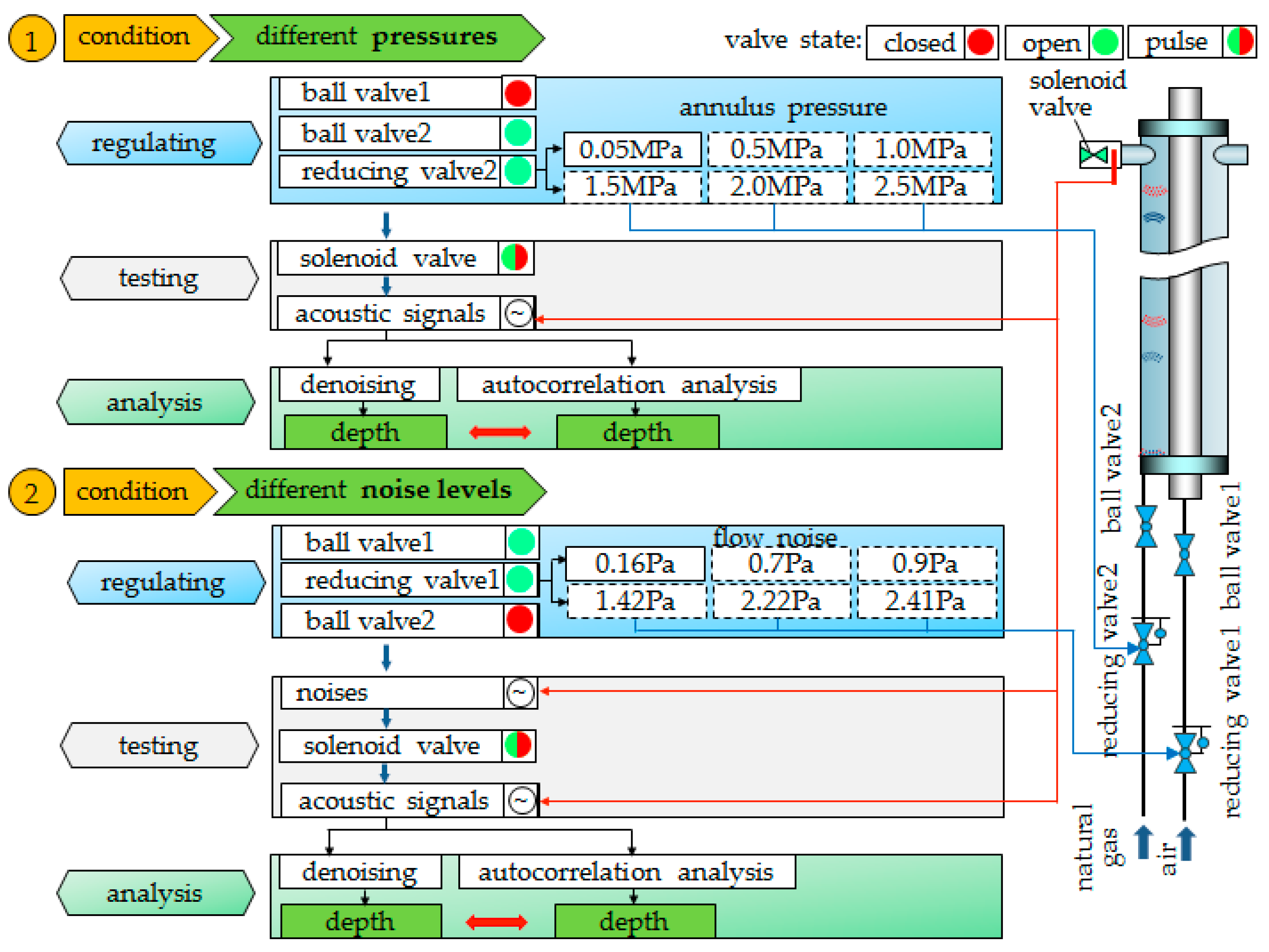
The experimental study is implemented under six annulus pressures which are 0.05, 0.50, 1.00, 1.50, 2.00 and 2.50 MPa, respectively, and six effective gas leak noise sound pressures which are 0.16, 0.70, 0.90, 1.42, 2.22 and 2.41 Pa, respectively. The experimental procedure is shown in Figure 9. Both the FFT-based filtering method and autocorrelation method are used to obtain the acoustic travel time. Figure 9 shows the experiment process of liquid level detection under different operating conditions. The acoustic travel time is obtained by using two data processing methods for every condition. One is the FFT-based filtering method which can decrease the noise of test signals and read the time difference between initial pulse and reflected pulse after noise reduction. Another is to adopt the ACF-based filtering method for the test signal and extract the signal cycle which is the travel time of the acoustic pulse. Crest Factor is introduced to evaluate the efficiency of the two algorithms in the feature extraction of reflected pulse from acoustic signals. Then the depth of the liquid level is computed by combing the acoustic travel time with the velocity. Finally, the validity and accuracy of the two methods are analyzed by comparing the estimation results with the actual liquid level depth.
4.3. Experimental Results and Analysis
4.3.1. Acoustic Signal Feature Extraction and Comparison Analysis under Different Annulus Pressures
Figure 10 shows the obtained signals denoised using FFT and ACF of different test acoustic signals under 2.50 MPa (a), 2.00 MPa (b), 1.50 MPa (c), 1.00 MPa (d), 0.50 MPa (e) and 0.05 MPa (f) annulus pressure. As shown in Figure 10, the peak amplitude of initial pulse Ai gradually decreases from 14.70 Pa to 4.24 Pa with the decreasing of annulus pressure from 2.50 MPa to 0.05 MPa. Therefore, as shown in Table 2, the reflected pulse amplitude of test signal, denoised signal and ACF also decrease. Particularly, the amplitude of the acoustic pulse is so weak that it is hard to be distinguished by FFT at 0.05 MPa annulus pressure, which is exhibited in Figure 10f.
However, the reflected pulse is easily identified by ACF. Normally, the computer software locates the liquid level by extracting the reflected pulse, so for an algorithm, the ability of identifying the acoustic pulse is what we are concerned about. In order to quantitatively reveal the identification ability of FFT and ACF, the Crest Factor is introduced as an evaluation index [46,47]. Crest Factor (aka Peak-to-Average Ratio) is defined as peak value divided by the effective value of a signal [48]:
where Xmax is the peak amplitude of the reflected pulse and Xrms is Root Mean Square (RMS) value of the analyzed signal. The larger the Crest Factor of the signal is, the better extracting effect of the processed signal is.
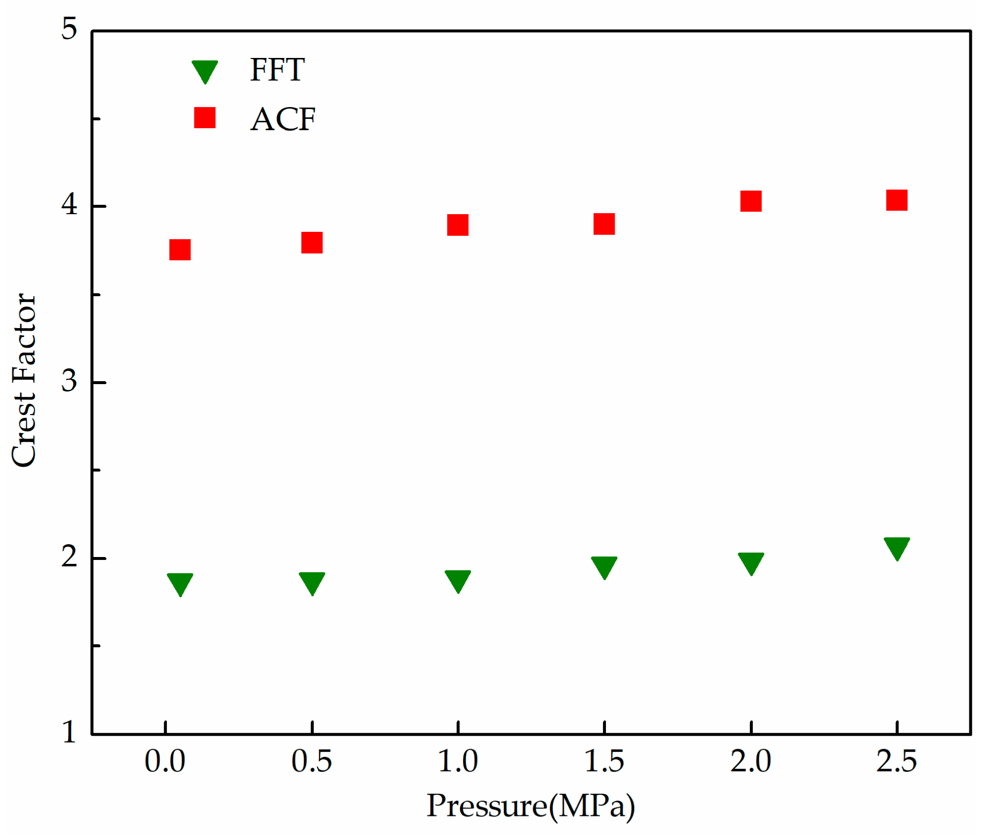
The comparison of Crest Factor of FFT between ACF is shown in Figure 11. As can be seen from the figure, the Crest Factor of the ACF of the test acoustic signal is significantly greater than that of FFT. For instance, the Crest Factors of FFT and ACF are 1.87 and 3.76, respectively, under 0.05 MPa annulus pressure. It’s worth mentioning that the Crest Factor of ACF is nearly twice as high as that of FFT, which reveals the superiority of the presented novel method.
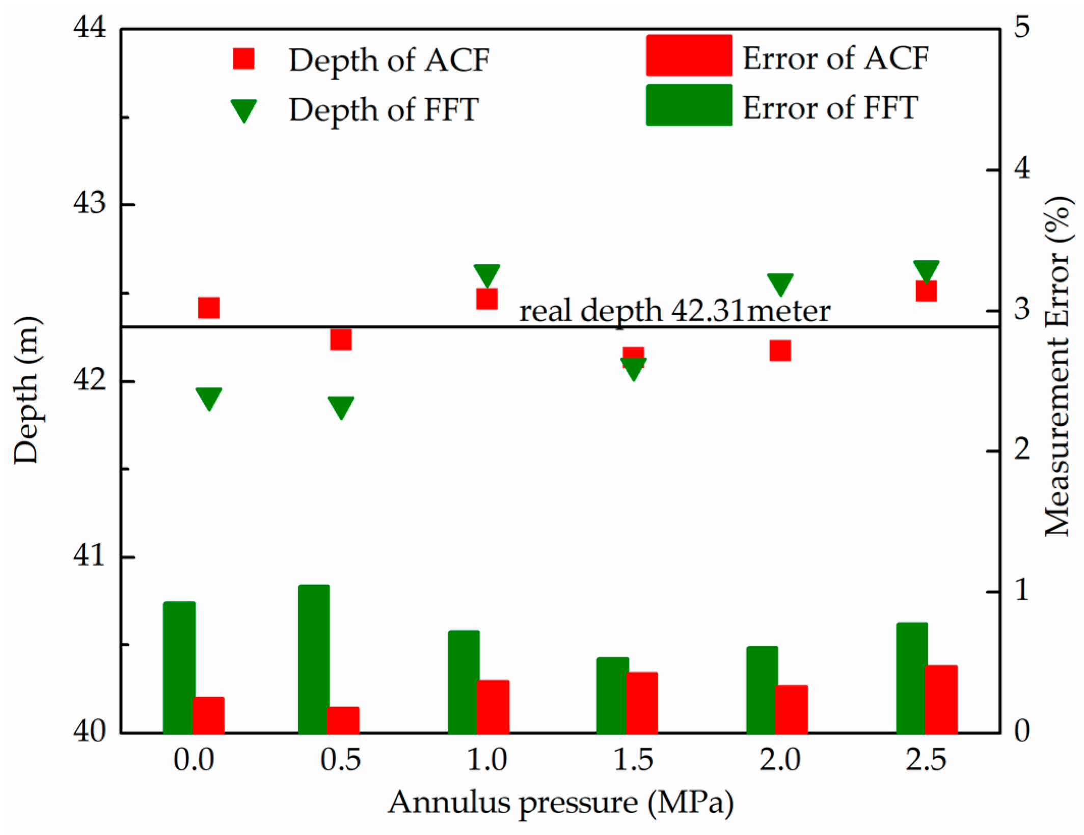
The comparison of liquid level determination between FFT and ACF under different annulus pressures is exhibited in the Figure 12. Compared with FFT, the depths of the liquid level are more close to the real values with ACF. The maximal measurement error reduces from 1.04% to 0.47% when the ACF is adopted, which shows that the new method is more accurate than FFT. The reason is that the time difference between initial pulse and reflected pulse is calculated considering more correlation by ACF, which can reduce the random error.
4.3.2. Acoustic Signal Feature Extraction and Comparison Analysis under Different Noise Levels
In this section, the liquid level is detected to evaluate the ability of the novel ACF method under different leak noise level conditions. Effective sound pressure pe which is defined as the square root of the mean of the squares of the acoustic pressure p is introduced as the criterion to describe the intensity of the leak noise. The pe is expressed as:
The flow rate of the compressed air is regulated by the reducing valve to generate noises, among which the effective sound pressure is 0.16, 0.70, 0.90, 1.42, 2.22 and 2.41 Pa, respectively. These noise levels are set according to the field data, as shown in Figure 13. Additionally, the annulus pressure is controlled at 0.05 MPa with an accuracy of ±1 kPa.
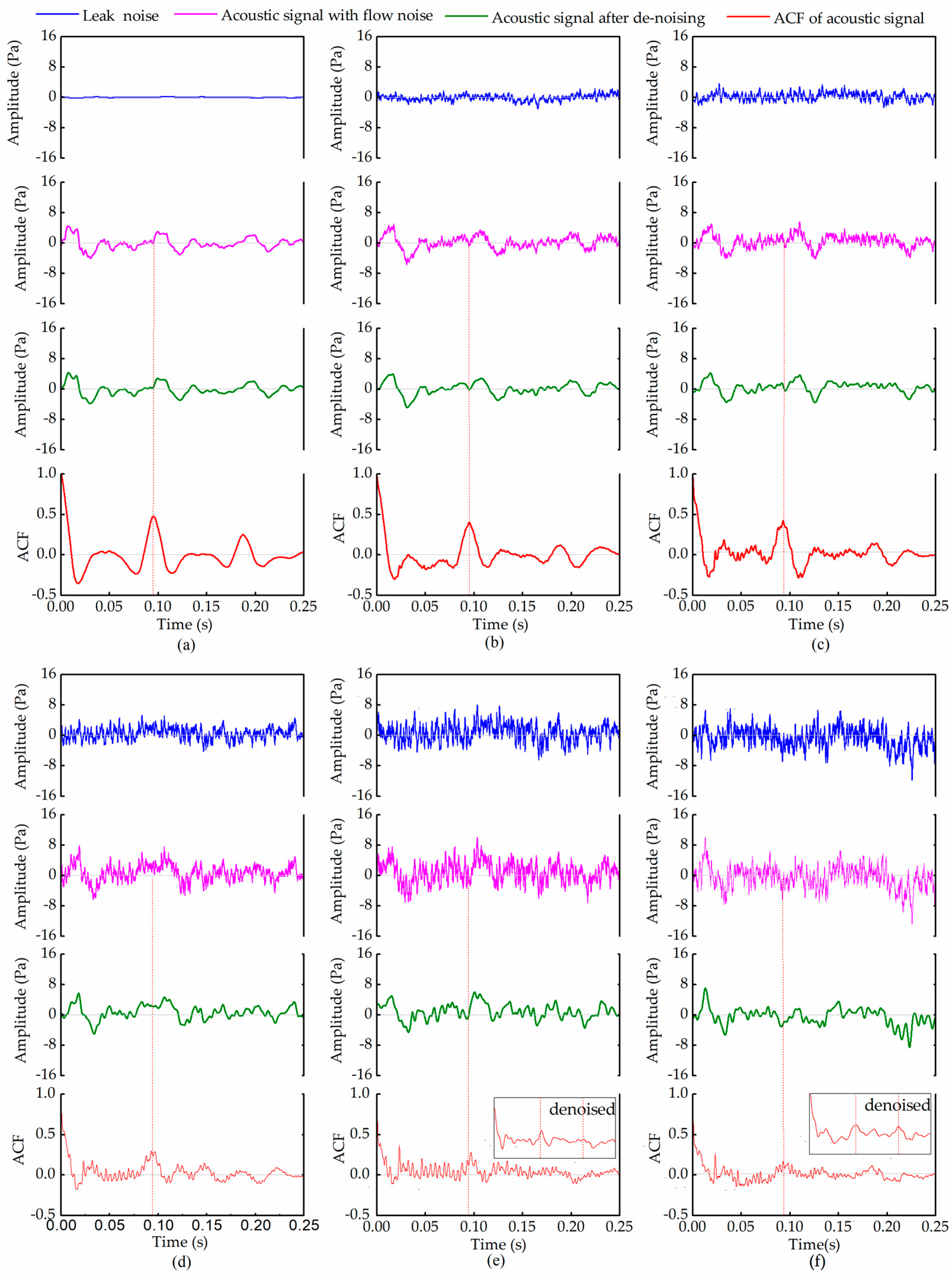
Firstly, the gas leak noises are measured separately, and then liquid levels with noises are detected. The waveforms of the noise signal, acoustic signal with noise, denoised acoustic signal with FFT, and ACF of the acoustic signal are shown in Figure 14. As shown in Figure 14, it is becoming increasingly hard to identify the reflections from liquid level with the increase of the effective sound pressure of the noise using FFT-based denoising method. In particular, the reflected pulse cannot be identified clearly using the FFT when the effective sound pressure of the noise is greater than 1.42 Pa. However, these reflected pulses can be clearly identified by ACF-based analysis, as shown in Figure 14d–f. Therefore, ACF-based analysis has a significant advantage in identifying the reflected pulse from the testing acoustic signal with leak noise compared to the conventional FFT-based filtering, which improves the anti-noise ability of the acoustic liquid level detection system.
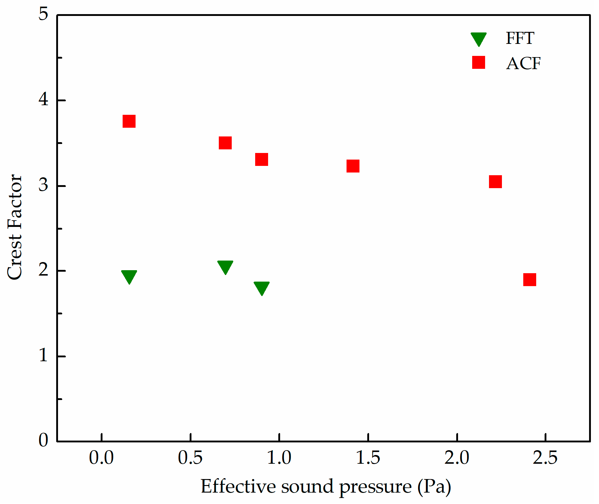
Figure 15 shows the comparison of Crest Factor of FFT and ACF under different noise levels. As can be seen from the figure, the Crest Factor of the ACF of the test acoustic signal is significantly greater than that of FFT. In particular, when the effective sound pressure of the noise is larger than 0.90 Pa, the reflected pulse cannot be identified from the denoised signal using the FFT, but ACF can do it.
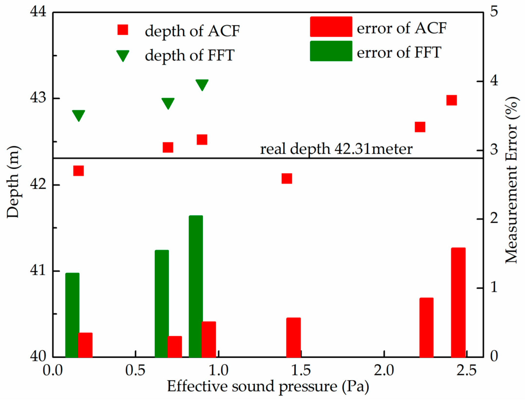
The comparison of liquid level determination between FFT and ACF under different noise levels is displayed in the Figure 16. Compared with FFT, the depths of the liquid level are also closer to practice than with ACF. The maximal measurement error reduces from 2.00% to 0.50% when the ACF is adopted, which shows that the new method is more accurate than FFT. The reason is that the low frequency noise can be filtered from acoustic wave signal by ACF, while it is impossible for FFT.
5. Field Application and Analysis
In order to verify the field application effect of the proposed novel method, a CSG well is selected as a case study for analysis.
5.1. Description of Field Test
The mentioned study has been done in Yangquan (Shanxi Province, China), which has one of the major coal bed methane block with an acreage of 2668 km2. A coal seam gas well is selected for the study because it is producing significant amount of gas. The calculated liquid level results are compared with result obtained from installed permanent pressure gauge. Figure 17 shows the typical well structure of a coal seam gas well in the field.
The acoustic liquid level determination system is installed at the wellhead of the tubing-production casing annulus. The detailed parameters of the well are listed in Table 3.
5.2. Results and Analysis
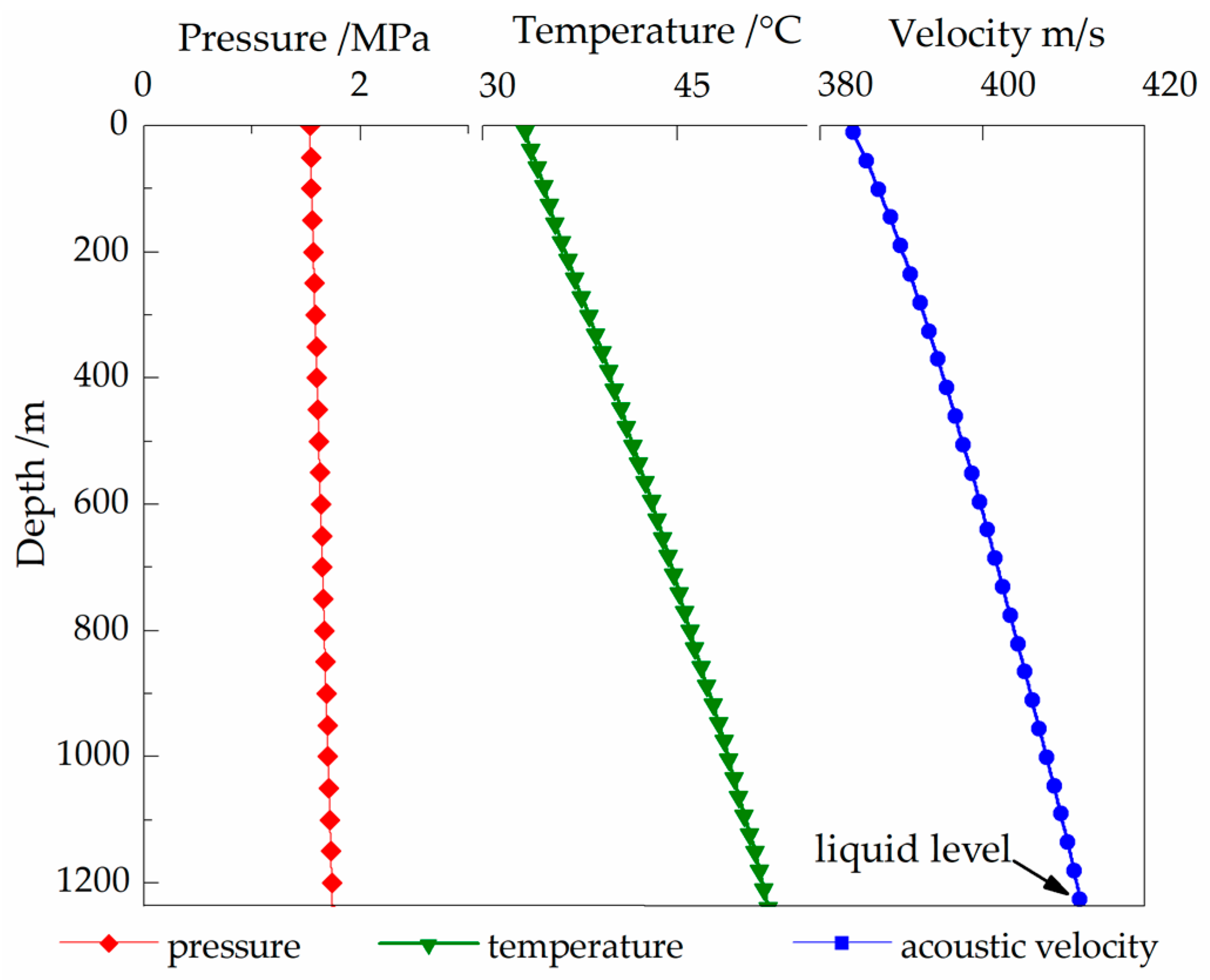
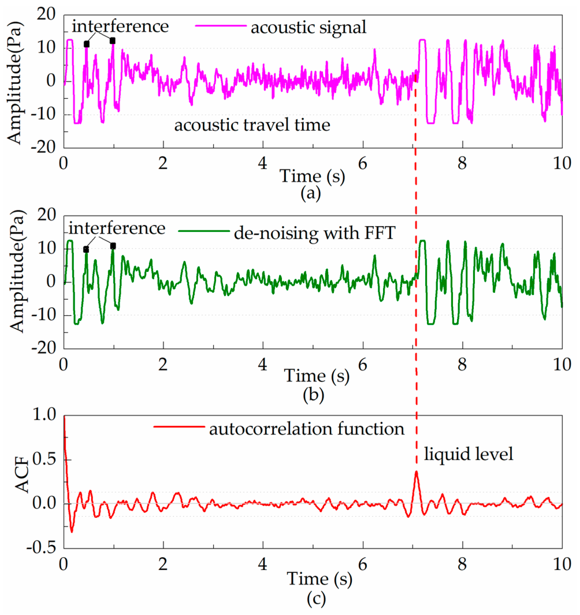
The test acoustic signal that contains much noise is shown in Figure 18a, which results in a difficulty to identify the acoustic pulse reflected from the liquid level. The de-noised acoustic signal using FFT is indicated in Figure 18b, which reduces some interference in the acoustic signal. However, some strong low frequency noise is still existing in the acoustic signal. The ACF of the acoustic signal with the novel method is shown in Figure 18c. The reflected pulse peak is observed at 7.06 s which is the round-trip time of acoustic propagation in the annulus. The corresponding Crest Factor of the test acoustic signal, de-noised acoustic signal and ACF are 2.79, 3.01 and 5.86, respectively, which reveals the advantages of the novel method in extracting the reflected signal by liquid level under high noise conditions.
Based on the iterative model mentioned in Section 3.3, the pressure, temperature and acoustic velocity distribution along the depth of the annulus are obtained as shown in Figure 19. The non-linear model of acoustic velocity is adopted to improve the accuracy of the measurement in the paper. In order to verify the accuracy between the FFT method and the ACF method, the annulus liquid level is detected by an installed permanent pressure gauges and the true depth is 1224.61 m. The measured depth of the liquid level with FFT is 1245.34 m and its measurement error is 1.70%. However, the measured depth of the liquid level with ACF is 1236.80 m and its measurement error is 1.00%, which verifies the accuracy of the novel method. Note that foam column exists up the surface of water if the gas well has a high production. The water/gas liquid level depth should be calculated by a theoretic calculation method based on the data of acoustic liquid level and wellhead pressure well depth which are obtained after “shut-in” and pressure “build-up” for few minutes [49].
6. Conclusions
A novel autocorrelation method has been developed in this study, and its ability to extract weak reflection pulse signals has been evaluated as well as accuracy for liquid level measurement through laboratory and field experiments. Some important conclusions can be drawn as follows:
- In the laboratory experiment, a comparative study was carried out to discuss the extraction ability and accuracy between the autocorrelation method and FFT under different sound pressures and noise levels. Compared to FFT-based filtering algorithm, the Crest Factor increases 1.88 and the maximal measurement error reduces from 1.04% to 0.47% under non-nosise conditoin when the autocorrelation method is adopted. In addition, the latent periodic characteristic of the reflected signal can be extracted with the autocorrelation method when the noise is larger than 1.42 Pa, which can not be obtained in FFT.
- In field experiments, the obtained Crest Factors are 3.01 and 5.86, respectively, using the two methods, which shows that the novel approach make liquid level reflection signal be better recognized by the testing system.
- Therefore, the new method can not only provide the theoretical guidance for the testing methods but also have the field application value on accurately and precisely detecting the liquid level of CSG wells.
The ACF-based acoustic liquid level determination method improves the measurement accuracy and noise immunity capability of the liquid level test system used in CSG wells. It provides a technical foundation for optimizing the well performance, avoiding coalbed formation damage and consequently reducing permeability. In the near future, the improved system can be better used for energy loss efficiency in the lifting and process monitoring in real time and adaptive control during drilling.
Acknowledgments
This work is supported by the National Key Research and Development Plan of China under Grant 2017YFC0804500. Special thanks are due to the anonymous reviewers for their useful comments and suggestions regarding the present paper.
Author Contributions
Each of the authors contributes on performing experiments and writing articles. Ximing Zhang is the main authors of this manuscript and this work was conducted under advisement of Jianchun Fan. Shengnan Wu and Di Liu helped to finish the experiments. All authors revised and approved the publication.
Conflicts of Interest
The authors declare no conflict of interest.
References
- Zhang, L.; Zhang, H.; Guo, H. A case study of gas drainage to low permeability coal seam. Int. J. Min. Sci. Technol. 2017, 27, 687–692. [Google Scholar] [CrossRef]
- Cao, Y.; Zhang, J.; Zhai, H.; Fu, G.; Tian, L.; Liu, S. CO2 gas fracturing: A novel reservoir stimulation technology in low permeability gassy coal seams. Fuel 2017, 203, 197–207. [Google Scholar] [CrossRef]
- Karacan, C.O. Best practice guidance for effective methane drainage and use in coal mines—United Nations Economic Commission for Europe Energy Series No: 31. Int. J. Coal Geol. 2014, 121, 35–36. [Google Scholar] [CrossRef]
- Qin, Y.; Wei, C.; Wang, G.X.; Rudolph, V.; Fu, X.; Wu, C. Fundamental studies and practice for enhanced coalbed methane technologies in China: A review. In Proceedings of the APCBM 2008 Symposium, Brisbane, Australia, 22–24 September 2008; pp. 1–31. [Google Scholar]
- Shen, J.; Qin, Y.; Wang, G.X.; Fu, X.; Wei, C.; Lei, B. Relative permeabilities of gas and water for different rank coals. Int. J. Coal Geol. 2011, 86, 266–275. [Google Scholar] [CrossRef]
- Schraufnagel, R.A.; McBane, R.A. Coalbed methane production. In Proceedings of the Annual Technical Conference and Exhibition, New Orleans, LA, USA, 25–28 September 1994; pp. 1–14. [Google Scholar]
- Durucan, S.; Ahsanb, M.; Shia, J.Q. Matrix shrinkage and swelling characteristics of European coals. Energy Procedia 2009, 1, 3055–3062. [Google Scholar] [CrossRef]
- Mitchell, T.R.; Leonardi, C.R. Micromechanical investigation of fines liberation and transport during coal seam dewatering. J. Nat. Gas Sci. Eng. 2016, 35, 1101–1120. [Google Scholar] [CrossRef]
- Tao, S.; Wang, Y.B.; Tang, D.Z.; Xu, H.; Lv, Y.M.; He, W.; Li, Y. Dynamic variation effects of coal permeability during the coalbed methane development process in the Qinshui Basin, China. Int. J. Coal Geol. 2012, 93, 16–22. [Google Scholar] [CrossRef]
- Lieberman, S. Automated continuous fluid level monitoring. In Proceedings of the SPE Production Operations Symposium, Oklahoma City, OK, USA, 16–19 April 2005; pp. 1–18. [Google Scholar]
- Palmer, I. Permeability changes in coal: Analytical modeling. Int. J. Coal Geol. 2009, 77, 119–126. [Google Scholar] [CrossRef]
- Li, P.; Chen, S.; Cai, Y.; Chen, J.; Li, J. Accurate TOF measurement of ultrasonic signal echo from the liquid level based on a 2-D image processing method. Neurocomputing 2016, 175, 47–54. [Google Scholar] [CrossRef]
- Schubert, J.J.; Wright, J.C. Early kick detection through liquid level monitoring in the wellbore. In Proceedings of the 1998 IADC/SPE Drilling Conference, Dallas, TX, USA, 3–6 March 1998; pp. 1–7. [Google Scholar]
- Godbey, J.K.; Ballard, B.G. Automatic Liquid Level Monitor. U.S. Patent 140410, 14 April 1980. [Google Scholar]
- McCoy, J.N.; Rowlan, O.L.; Becker, D.; Podio, A.L. Applications of acoustic liquid level measurements in gas wells. In Proceedings of the 2006 SPE Annual Technical Conference and Exhibition, San Antonio, TX, USA, 24–27 September 2006; pp. 1–16. [Google Scholar]
- Peng, G.L.; He, J.; Yang, S.P.; Zhou, W.Y. Application of the fiber-optic distributed temperature sensing for monitoring the liquid level of producing oil wells. Measurement 2014, 58, 130–137. [Google Scholar] [CrossRef]
- McCoy, J.N.; Rowlan, O.L.; Becker, D.; Podio, A.L. Advanced techniques for acoustic liquid level determination. In Proceedings of the Petroleum Society’s Canadian International Petroleum Conference, Calgary, AB, Canada, 11–13 June 2002; pp. 1–14. [Google Scholar]
- Rowlan, O.L.; McCoy, J.N.; Becker, D.; Podio, A.L. Advanced techniques for acoustic liquid-level determination. In Proceedings of the SPE Production and Operations Symposium, Oklahoma City, OK, USA, 22–25 March 2003; pp. 1–12. [Google Scholar]
- Taylor, C.; Rowlan, L.; McCoy, J. Acoustic techniques to monitor and troubleshoot gas-lift wells. In Proceedings of the SPE Western North American and Rocky Mountain Joint Regional Meeting, Denver, CO, USA, 16–18 April 2014; pp. 1–10. [Google Scholar]
- Clarkson, C.; Bustin, M. Coalbed methane: Current evaluation methods, future technical challenges. In Proceedings of the SPE Unconventional Gas Conference, Pittsburgh, PA, USA, 23–25 February 2010; pp. 1–13. [Google Scholar]
- Bhargava, V.; Sethi, A.; Singh, S.; Chellani, I. A case study—determination of accurate liquid level and its applications in CBM wells. In Proceedings of the SPE Oil and Gas India Conference and Exhibition, Mumbai, India, 24–26 November 2015; pp. 1–8. [Google Scholar]
- McCoy, J.; Podio, A.L.; Rowlan, L.; Garrett, M. Acoustic foam depression tests. In Proceedings of the the 48th Annual Technical Meeting of the Petroleum Society, Calgary, AB, Canada, 8–11 June 1997; pp. 1–13. [Google Scholar]
- Han, G.Q.; Ling, K.G.; Zhang, H. Smart de-watering and production system through real-time water level surveillance for Coal-Bed Methane wells. J. Nat. Gas Sci. Eng. 2016, 31, 769–778. [Google Scholar] [CrossRef]
- The Application of the Realtime Annulus Liquid Level Determation System. Available online: http://www.gtpetro.com/unitermtech/gtp_unitech_lianxuyemian.html (accessed on 12 September 2015).
- Shi, J.Q.; Durucan, S. A model for changes in coalbed permeability during primary and enhanced recovery. SPE Reserv. Eval. Eng. 2005, 8, 291–299. [Google Scholar] [CrossRef]
- Ernest, J.H.; Evans, D.M.; Fasching, G.E. Wireless Remote Liquid Level Detector and Indicator for Well Testing. U.S. Patent 569087, 18 June 1985. [Google Scholar]
- Ramy, H.J. Wellbore heat transmission. J. Pet. Technol. 1962, 14, 427–435. [Google Scholar] [CrossRef]
- Hasan, A.R.; Kabir, C.S. Heat transfer during two phase flow in wellbore: Part 1-formation temperature. In Proceedings of the 66th Annual Technical Conference and Exhibition of the Society of Petroleum Engineers, Dallas, TX, USA, 6–9 October 1991; pp. 469–478. [Google Scholar]
- Adams, A.J. How to design for annulus fluid heat-up. In Proceedings of the 66th Annual Technical Conference and Exhibition of the Society of Petroleum Engineers, Dallas, TX, USA, 6–9 October 1991; pp. 529–540. [Google Scholar]
- Guan, Z.; Zhang, B.; Wang, Q.; Liu, Y.; Xu, Y.; Zhang, Q. Design of thermal-insulated pipes applied in deepwater well to mitigate annular pressure build-up. Appl. Therm. Eng. 2016, 98, 129–136. [Google Scholar] [CrossRef]
- Liu, J.; Fan, H.; Peng, Q.; Deng, S.; Kang, B.; Ren, W. Research on the prediction model of annular pressure buildup in subsea wells. J. Nat. Gas Sci. Eng. 2015, 27, 1677–1683. [Google Scholar] [CrossRef]
- Savidge, J.L.; Starling, K.E.; McFall, R.L. Sound speed of natural gas. In Proceedings of the SPE Gas Technology Symposium, Dallas, TX, USA, 13–15 June 1988. [Google Scholar]
- Ohno, J.; Yashiro, H. Method and Apparatus for Measuring Water Level in a Well. U.S. Patent 4621264A, 4 November 1986. [Google Scholar]
- Thomas, L.; Hankinson, R.; Phillips, K. Determination of acoustic velocities for natural gas. J. Pet. Technol. 1970, 22, 889–895. [Google Scholar] [CrossRef]
- Starling, K.E.; Savidge, J.L. Compressibility Factors of Natural Gas and Other Related Hydrocarbon Gases, 2nd ed.; American Gas Association: Washington, DC, USA, 1992. [Google Scholar]
- Aly, F.A.; Lee, L.L. Self-consistent equations for calculating the ideal gas heat capacity, enthalpy, and entropy. Fluid Phase Equilib. 1981, 6, 169–179. [Google Scholar] [CrossRef]
- Ahmadi, P.; Chapoy, A.; Tohidi, B. Density, speed of sound and derived thermodynamic properties of a synthetic natural gas. J. Nat. Gas Sci. Eng. 2017, 40, 249–266. [Google Scholar] [CrossRef]
- Alive, I.N.; Alhanati, F.J.S.; Shoham, O. A unified model for predicting flowing temperature distribution in wellbores and pipelines. SPE Prod. Eng. 1992, 11, 363–367. [Google Scholar]
- Moss, J.T.; White, P.D. How to calculate temperature profiles in a water-injection well. Oil Gas J. 1959, 57, 174. [Google Scholar]
- Sagar, R.; Doty, D.R.; Schmidt, Z. Predicting temperature profiles in a flowing well. SPE Prod. Eng. 1991, 11, 441–448. [Google Scholar] [CrossRef]
- Jin, Y.; Haixiong, T.; Zhengli, L.; Liping, Y.; Xiaolong, H.; De, Y.; Ruirui, T. Prediction model of casing annulus pressure for deepwater. Pet. Explor. Dev. 2013, 40, 661–664. [Google Scholar]
- Zheng, X.; Duan, C.; Yan, Z.; Ye, H.; Wang, Z.; Xia, B. Equivalent circulation density analysis of geothermal well by coupling temperature. Energies 2017, 10, 268. [Google Scholar] [CrossRef]
- Fattah, S.A.; Zhu, W.P.; Ahmad, M.O. An approach to formant frequency estimation at low signal-to-noise ratio. In Proceedings of the 2007 IEEE International Conference on Acoustics, Speech and Signal Processing (ICASSP 2007), Honolulu, HI, USA, 15–20 April 2007; pp. 469–472. [Google Scholar]
- Fattah, S.A.; Zhu, W.P.; Ahmad, M.O. An approach to ARMA system identification at a very low signal-to-noise ratio. In Proceedings of the IEEE International Conference on Acoustics, Speech and Signal Processing, Philadelphia, PA, USA, 18–23 March 2005; pp. 113–116. [Google Scholar]
- Gao, Y.; Brennan, M.J.; Joseph, P.F.; Muggleton, J.M.; Hunaidi, O. A model of the correlation function of leak noise in buried plastic pipes. J. Sound Vib. 2004, 277, 133–148. [Google Scholar] [CrossRef]
- Cai, B.; Liu, H.; Xie, M. Bayesian networks in fault diagnosis. IEEE Trans. Ind. Inform. 2017, 13, 2227–2240. [Google Scholar] [CrossRef]
- Cai, B.; Liu, H.; Xie, M. A real-time fault diagnosis methodology of complex systems using object-oriented Bayesian networks. Mech. Syst. Signal Process. 2017, 80, 31–44. [Google Scholar] [CrossRef]
- Nair, M.V.D.; Giofré, R.; Colantonio, P.; Giannini, F. Sequential asymmetric superposition windowing for Crest Factor Reduction and its effects on Doherty power amplifier. In Proceedings of the 2015 Integrated Nonlinear Microwave and Millimetre-Wave Circuits Workshop, Taormina, Italy, 1–2 October 2015; pp. 1–3. [Google Scholar]
- Khasanov, M.M.; Krasnov, V.; Khabibullin, R.; Pashali, A.; Semenov, A.A. New method for fluid level depression test interpretation based on modern multiphase flow calculation techniques. In Proceedings of the Society of Petroleum Engineers, Barcelona, Spain, 14–17 June 2010; pp. 1–10. [Google Scholar]
Figure 1.
Schematic diagram of acoustic level measurement.

Figure 2.
Computational grid of acoustic propagate in annulus.

Figure 3.
Schematic diagram of heat conduction through the radial direction.
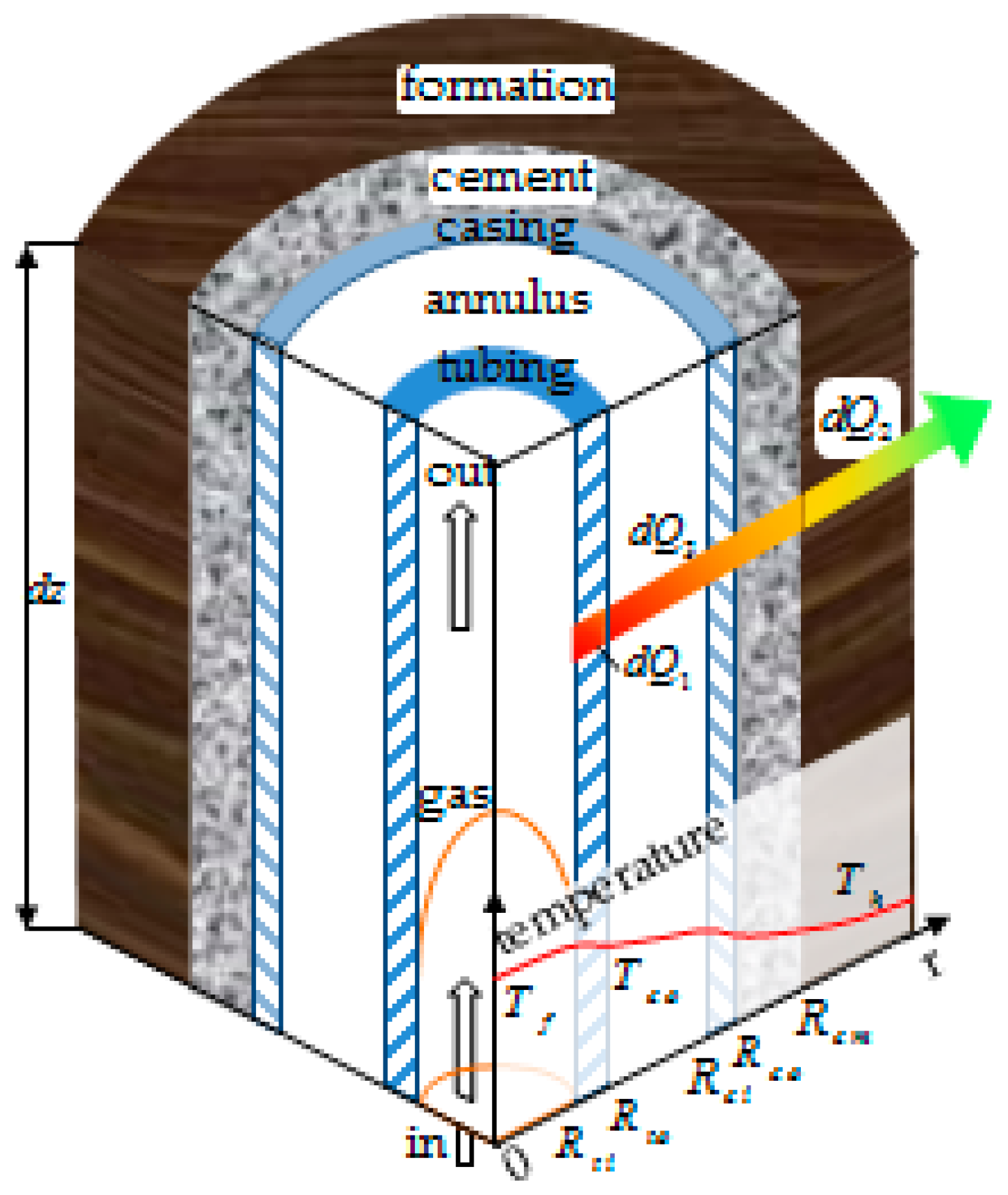
Figure 4.
Time domain (a) and frequency domain (b) of the test acoustic signal.
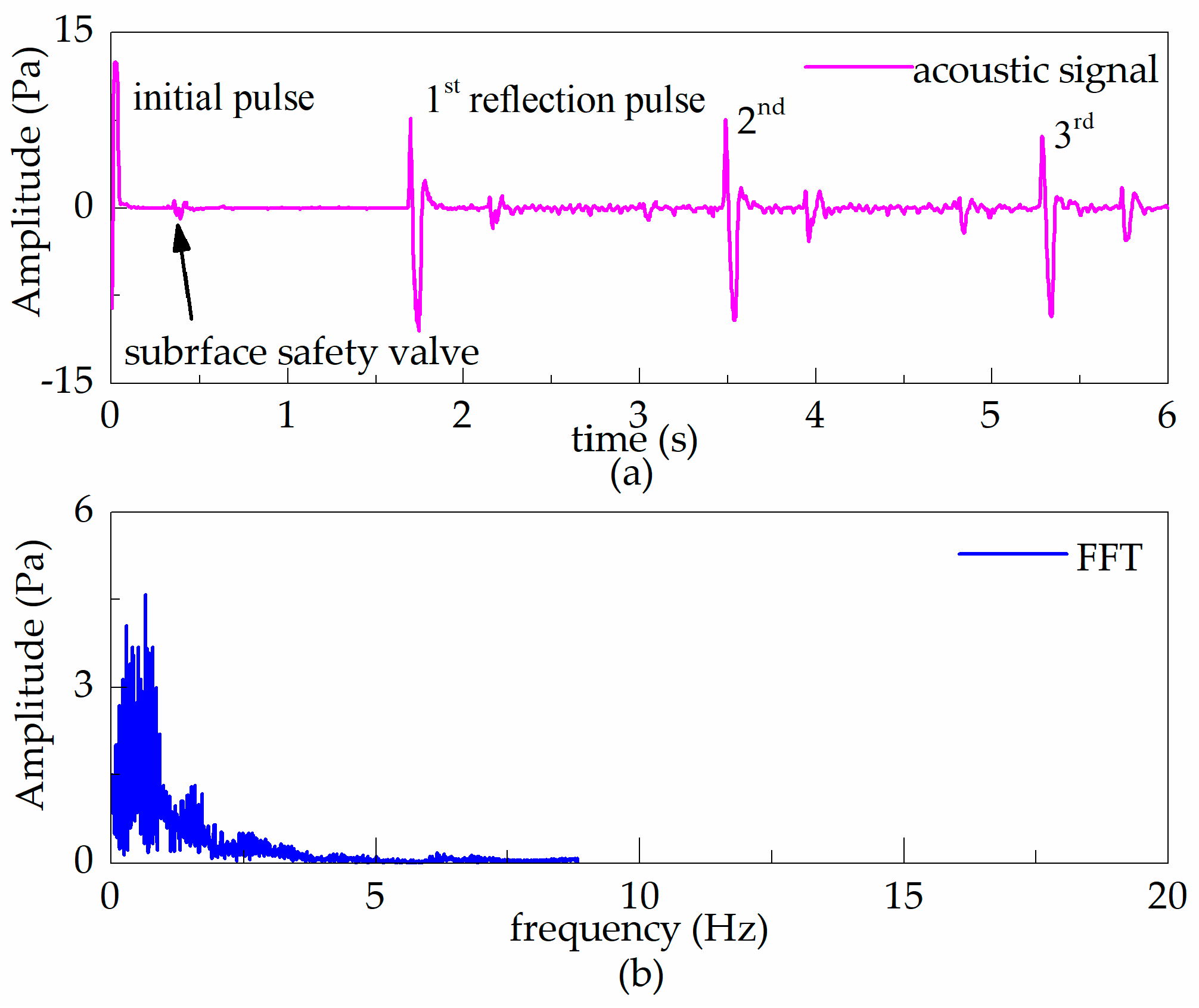
Figure 5.
Schematic of autocorrelation detection.

Figure 6.
Original and ACF of the test acoustic signal.

Figure 7.
Flow chart of the liquid level calculation.
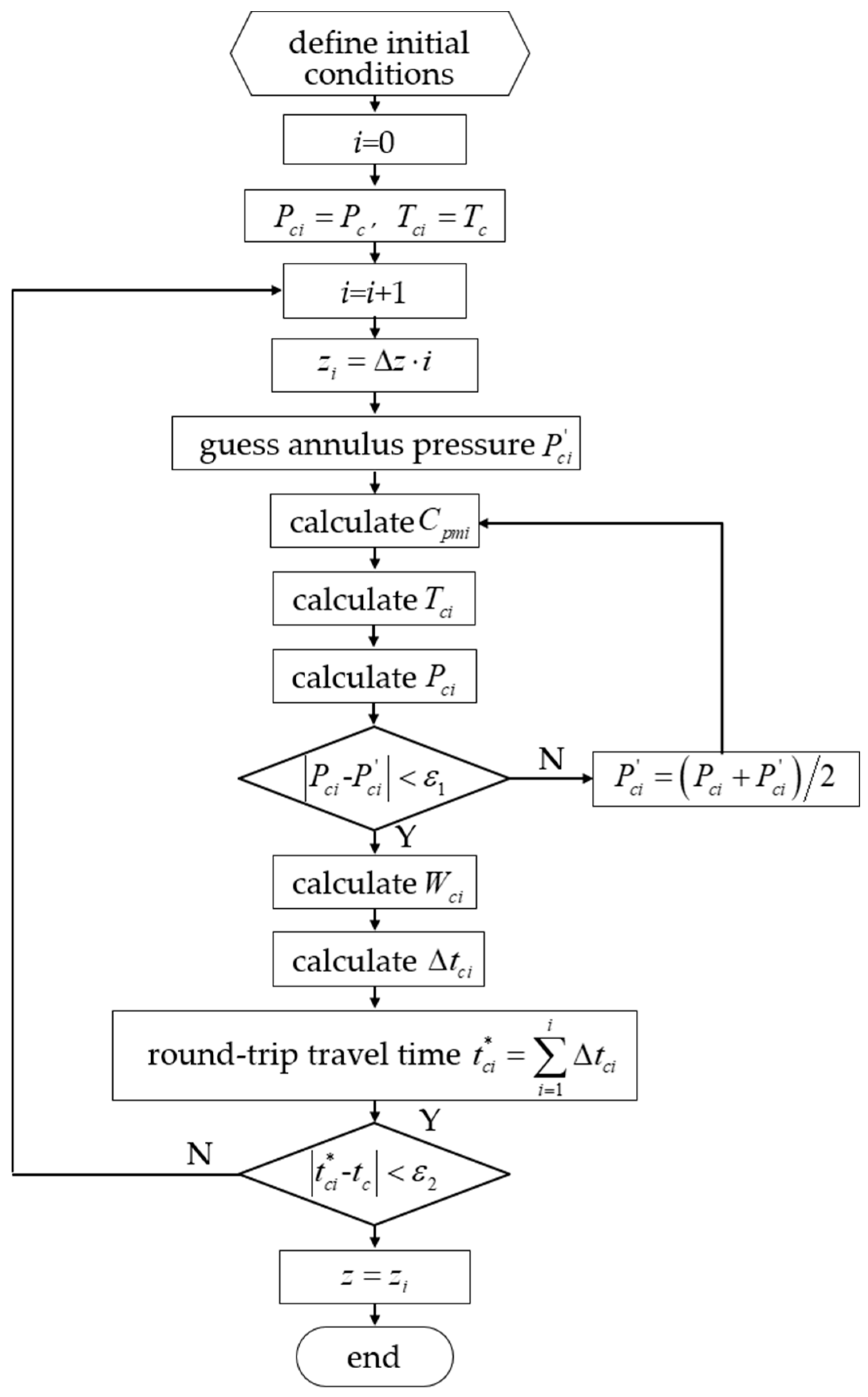
Figure 8.
Experimental devices of the liquid level test.

Figure 9.
Experimental process of liquid level detection under different operating conditions.

Figure 10.
Performance comparison for FFT and ACF under different annulus pressures of (a) 2.50 MPa; (b) 2.00 MPa; (c) 1.50 MPa; (d) 1.00 MPa; (e) 0.50 MPa; (f) 0.05 MPa.
Figure 10.
Performance comparison for FFT and ACF under different annulus pressures of (a) 2.50 MPa; (b) 2.00 MPa; (c) 1.50 MPa; (d) 1.00 MPa; (e) 0.50 MPa; (f) 0.05 MPa.
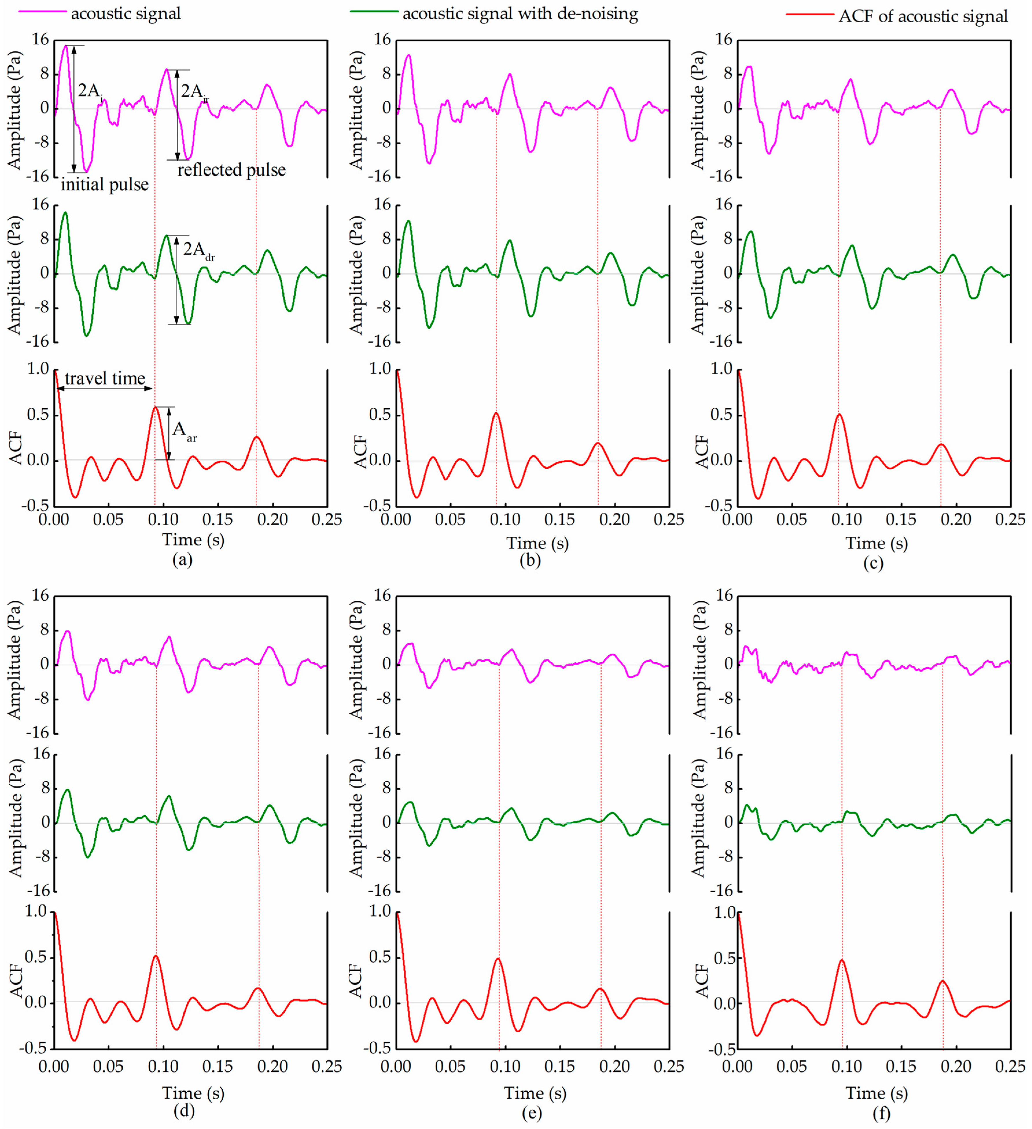
Figure 11.
Comparison of Crest Factor of the signal between FFT and ACF under different annulus pressures.
Figure 11.
Comparison of Crest Factor of the signal between FFT and ACF under different annulus pressures.

Figure 12.
Comparison of liquid level determination between FFT and ACF under different annulus pressures.
Figure 12.
Comparison of liquid level determination between FFT and ACF under different annulus pressures.

Figure 13.
Noise test at the wellhead of CSG wells. Diagram of noise test (a); Time domain (b) and frequency domain (c) of the test acoustic signal.
Figure 13.
Noise test at the wellhead of CSG wells. Diagram of noise test (a); Time domain (b) and frequency domain (c) of the test acoustic signal.
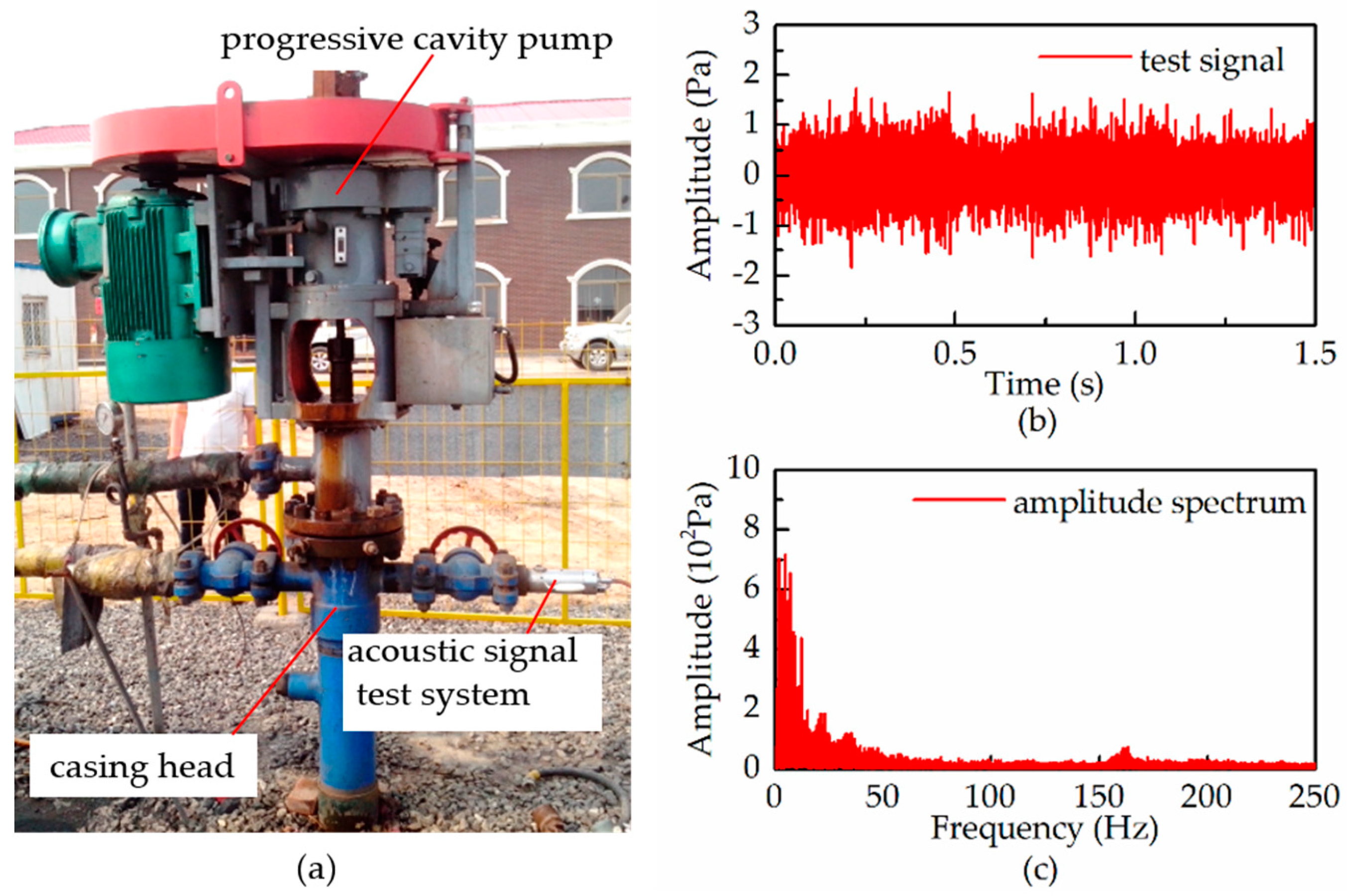
Figure 14.
Waveform of FFT and ACF under different annulus pressures of (a) 0.16 Pa; (b) 0.70 Pa; (c) 0.90 Pa; (d) 1.40 Pa; (e) 2.20 Pa; (f) 2.40 Pa.
Figure 14.
Waveform of FFT and ACF under different annulus pressures of (a) 0.16 Pa; (b) 0.70 Pa; (c) 0.90 Pa; (d) 1.40 Pa; (e) 2.20 Pa; (f) 2.40 Pa.

Figure 15.
Comparison of Crest Factor of the signal between FFT and ACF under different noise levels.
Figure 15.
Comparison of Crest Factor of the signal between FFT and ACF under different noise levels.

Figure 16.
Comparison of liquid level determination between FFT and ACF under different noise levels.
Figure 16.
Comparison of liquid level determination between FFT and ACF under different noise levels.

Figure 17.
Schematic of the test CSG well.
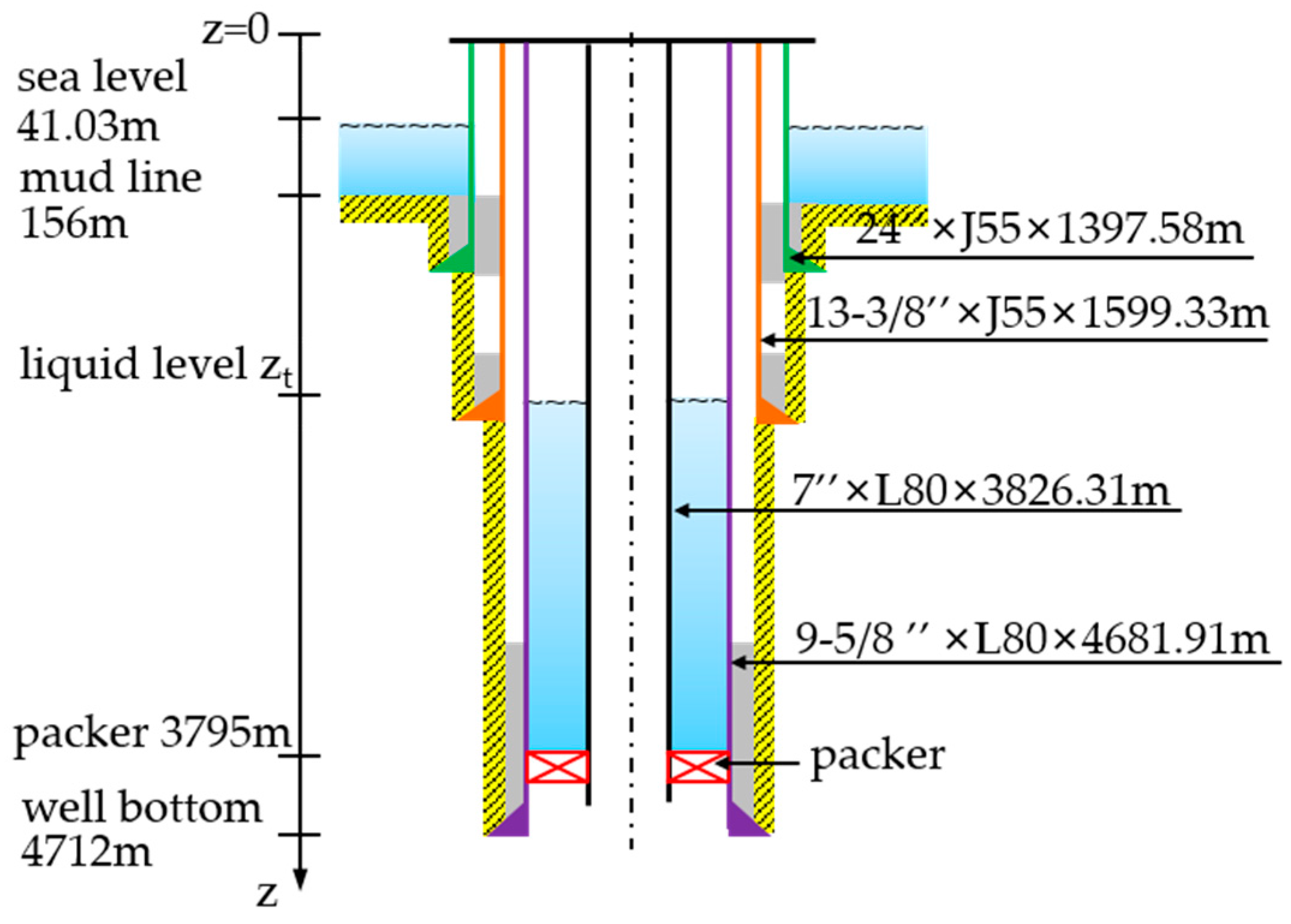
Figure 18.
Waveform of test acoustic signal (a); acoustic signal with FFT-based denoising method (b); ACF of the acoustic signal (c).
Figure 18.
Waveform of test acoustic signal (a); acoustic signal with FFT-based denoising method (b); ACF of the acoustic signal (c).

Figure 19.
Pressure, temperature and acoustic velocity distribution in annulus.

Table 1.
The main parameters of the experimental devices.
| Subsystem | Item | Parameter |
|---|---|---|
| Simulation wellbore | tubing specifications | Φ 73.00 × 5.51 mm |
| casing specifications | Φ 139.70 × 6.20 mm | |
| length of annulus | 42.13 m | |
| Acoustic liquid level detection | pressure range | 0.00 to 57.30 kPa |
| frequency range | 0.10 to 10,000 Hz | |
| Annulus pressure control system | gas components | 95.12% CH4, 2.55% CO2, 1.83% C2H6 and 0.45% C3H8 |
| Gas supply system | maximum flow | 1000 stand m3/day |
Table 2.
Reflected pulse variation under different annulus pressures.
| Annulus Pressure (MPa) | Amplitude (Pa) | |||
|---|---|---|---|---|
| 2.50 | 14.70 | 10.51 | 14.42 | 0.59 |
| 2.00 | 12.66 | 9.11 | 12.50 | 0.53 |
| 1.50 | 10.21 | 7.60 | 10.08 | 0.52 |
| 1.00 | 8.00 | 6.45 | 7.90 | 0.51 |
| 0.50 | 5.20 | 3.82 | 5.10 | 0.49 |
| 0.05 | 4.24 | 3.01 | 4.08 | 0.48 |
Table 3.
Main parameters of the test well.
| Item | Parameters |
|---|---|
| diameter of tubing (mm) | Φ73.00 × 5.51 |
| diameter of casing (mm) | Φ139.70 × 6.20 |
| formation temperature (°C) | 78.23 |
| geothermal gradient (°C/100 m) | 3.67 |
| setting depth of pressure gauge (m) | 1340.17 |
| tubing temperature (°C) | 33.27 |
| annulus temperature (°C) | 30.20 |
| annulus pressure (MPa) | 1.53 |
| density of annular fluid (g/cm3) | 0.95 |
| producing of gas (stand m3/day) | 3000.00 |
© 2017 by the authors. Licensee MDPI, Basel, Switzerland. This article is an open access article distributed under the terms and conditions of the Creative Commons Attribution (CC BY) license (http://creativecommons.org/licenses/by/4.0/).
Share and Cite
MDPI and ACS Style
Zhang, X.; Fan, J.; Wu, S.; Liu, D. A Novel Acoustic Liquid Level Determination Method for Coal Seam Gas Wells Based on Autocorrelation Analysis. Energies 2017, 10, 1961. https://doi.org/10.3390/en10121961
AMA Style
Zhang X, Fan J, Wu S, Liu D. A Novel Acoustic Liquid Level Determination Method for Coal Seam Gas Wells Based on Autocorrelation Analysis. Energies. 2017; 10(12):1961. https://doi.org/10.3390/en10121961
Chicago/Turabian StyleZhang, Ximing, Jianchun Fan, Shengnan Wu, and Di Liu. 2017. "A Novel Acoustic Liquid Level Determination Method for Coal Seam Gas Wells Based on Autocorrelation Analysis" Energies 10, no. 12: 1961. https://doi.org/10.3390/en10121961
Note that from the first issue of 2016, this journal uses article numbers instead of page numbers. See further details here.