Shale Gas Content Calculation of the Triassic Yanchang Formation in the Southeastern Ordos Basin, China

1
School of Earth Sciences and Resources, China University of Geosciences, Beijing 100083, China
2
School of Earth and Space Sciences, Peking University, Beijing 100871, China
3
Oil and Gas Research Center, Peking University, Beijing 100871, China
4
Key Laboratory of Shale Gas and Geoengineering, Institute of Geology and Geophysics, Chinese Academy of Sciences, Beijing 100029, China
5
Institutions of Earth Science, Chinese Academy of Sciences, Beijing 100029, China
*
Author to whom correspondence should be addressed.
Energies 2017, 10(12), 1949; https://doi.org/10.3390/en10121949
Submission received: 28 September 2017
/
Revised: 15 November 2017
/
Accepted: 20 November 2017
/
Published: 24 November 2017
Abstract
:Shale gas content is the key parameter for shale gas potential evaluation and favorable area prediction. Therefore, it is very important to determine shale gas content accurately. Generally, we use the US Bureau of Mines (USBM) method for coal reservoirs to calculate the gas content of shale reservoirs. However, shale reservoirs are different from coal reservoirs in depth, pressure, core collection, etc. This method would inevitably cause problems. In order to make the USBM method more suitable for shale reservoirs, an improved USBM method is put forward on the basis of systematic analysis of core pressure history and temperature history during shale gas degassing. The improved USBM method modifies the calculation method of the gas loss time, and determines the temperature balance time of water heating. In addition, we give the calculation method of adsorption gas content and free gas content, especially the new method of calculating the oil dissolved gas content and water dissolved gas content that are easily neglected. We used the direct method (USBM and the improved USBM) and the indirect method (including the calculation of adsorption gas, free gas and the dissolved gas method) to calculate the shale gas content of 16 shale samples of the Triassic Yanchang Formation in the Southeastern Ordos Basin, China. The results of the improved USBM method show that the total shale gas content is high, with an average of 3.97 m3/t, and the lost shale gas content is the largest proportion with an average of 62%. The total shale gas content calculated by the improved USBM method is greater than that of the USBM method. The results of the indirect method show that the total shale gas content is large, with an average of 4.11 m3/t, and the adsorption shale gas content is the largest proportion with an average of 71%. The oil dissolved shale gas content which should be paid attention to accounts for about 7.8%. The discrepancy between the direct method and indirect method is reduced by using the improved USBM method, and the improved USBM method could be more practical and accurate than the USBM method.
1. Introduction
With the successful exploitation of shale gas in North America [1,2,3], many Chinese scholars have begun to study China’s shale gas resources, and have found that China has a huge amount of shale gas resources [4,5,6,7]. In recent years, Chinese enterprises have started industrial exploitation of shale gas in Sichuan Province and other regions, and obtained high shale gas production [8,9,10,11]. Shale gas has become one of the most popular unconventional oil and gas resources in China today [12,13,14]. Shale gas content is the key parameter for shale gas potential evaluation and favorable area prediction. Therefore, it is very important to determine shale gas content accurately [15,16,17,18,19,20]. So far, there is no uniform industry standard and experimental technology for measuring shale gas content. In general, shale gas content measurement methods can be divided into two types: the direct method and indirect method [21,22]. The direct method (the degassing method) determines shale gas content through direct degassing experiments of fresh shale samples on the drilling site. The shale gas content of the direct method is composed of three parts: degassing shale gas content, lost shale gas content and residual shale gas content. Lost shale gas is a gas that escapes from the shale core during core lifting. However, the direct method is initially based on the coal reservoir model. Coal reservoirs are different from shale reservoirs. Calculating the lost shale gas content using the direct method may result in great errors. The accuracy of the direct method for shale reservoirs, however, is dependent on correctly estimating the lost shale gas content [23]. Therefore, how to calculate the accurate lost shale gas content has become the research focus of the direct method. Normally, we use the US Bureau of Mines (USBM) method [24], the Smith–Williams method [25,26], the curve fitting method [27], the flow simulation method [23], etc., to restore the lost shale gas content. As an industrial measurement standard for coal bed methane content in the United States and China, the USBM method is widely used because of its simple operability and high accuracy. The indirect method includes the methane isothermal adsorption method, the log interpretation method and the statistical analysis method. The adsorption shale gas content and the adsorption capacity of shale are studied using the Langmuir model [19,28,29]. The log interpretation method refers to the calculation of shale gas content by using many log response characteristics [30,31]. The statistical analysis method is to calculate the shale gas content by using the main geological factors that affect shale gas content [32,33]. Generally speaking, the indirect method can obtain abundant information about shale gas content, and the direct method is the most common and accurate test method at present.
The USBM method was originally applied to coal reservoirs. However, shale reservoirs are different from coal reservoirs in depth, pressure, core collection, etc. The depth of China’s coal reservoirs is generally 300 m to 1500 m [34,35,36], while the depth of China’s shale reservoirs is generally between 1500 m and 4500 m [4,6,36]. The pressure of China’s shale reservoirs is generally high or low pressure, while normally the pressure of China’s coal reservoirs is low [6,36]. In addition, the time of coal core collection by wire coring is much shorter than the time of shale core collection by drill pipe coring. These differences in depth, pressure and core collection may lead to errors in calculating the lost shale gas content. Therefore, if applied to shale reservoirs directly, the USBM method would inevitably cause problems. In order to make the USBM method more suitable for shale reservoirs, an improved USBM method is put forward. The improved USBM method is based on a systematic analysis of core pressure history and temperature history during shale gas degassing. The newly improved USBM method modifies the calculation method of the gas loss time, and determines the temperature balance time of water heating. Meanwhile, we also provide a calculation method for adsorption shale gas content and free shale gas content. We especially created the new method to calculate the oil-dissolved shale gas content and water-dissolved shale gas content, which are easily neglected. We used the direct method (USBM and the improved USBM) and the indirect method (adsorption gas, free gas and dissolved gas) to calculate the shale gas content of 16 shale samples from the Triassic Yanchang Formation in the Southeastern Ordos Basin, China.
2. Experimental Methods
2.1. On-Site Shale Degassing Experiments
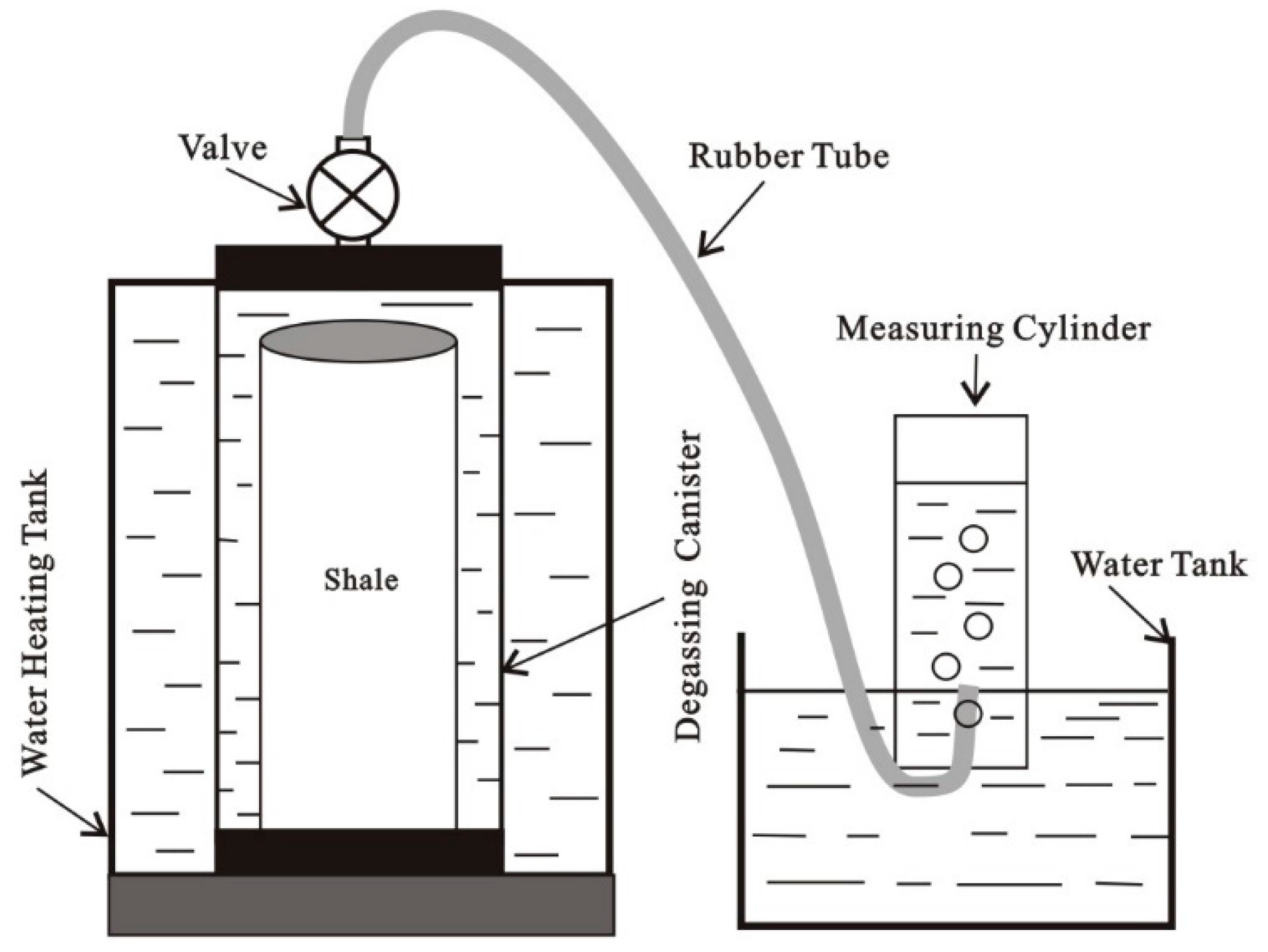
In order to obtain an accurate degassing shale gas content and residual shale gas content, on-site shale degassing experiments were conducted on 16 shale samples of the Triassic Yanchang Formation in the Southeastern Ordos Basin, China. Degassing shale gas is a gas that is degassed from shale. Degassing shale gas content is measured by a water heating degassing instrument via means of downward drainage counts. The water-heating degassing instrument includes a water-heating tank, degassing canister, water tank, measuring cylinder, valve and rubber tube, etc. (Figure 1). The experimental process consists of three parts: waiting for core lifting, core loading and data recording. When waiting for core lifting, the temperatures in the water heating tank and degassing canister rise and are then maintained at the actual formation temperature. Core loading refers to weighing these drilled shale core samples and loading them into degassing canisters as soon as possible. Data recording refers to the process of recording the cumulative degassing gas volume and degassing time. Residual shale gas is the gas remaining in the dead pores of shale. Dead pores refer to disconnected pores, and shale gas cannot escape from dead pores. Residual shale gas content is measured by a ball-milling machine which shatters shale samples and releases the residual shale gas from shale samples. The experiment process consists of three parts: sample weighing, crushing and data recording. We took about five minutes to crush a sample. When the pressure of ball milling machine no longer increases, we believe that all the residual gas has been released. Then we recorded the residual shale gas volume by means of downward drainage counts.
2.2. Methane Isothermal Sorption Measurements
In order to obtain accurate adsorption shale gas content and evaluate the methane adsorption capacity of shale, methane isothermal sorption measurements were conducted on 16 shale samples from the Triassic Yanchang Formation in the Southeastern Ordos Basin, China. The methane isothermal sorption measurements were performed on FY–KT1000 isothermal adsorption apparatus (Bangda New Technology co., Renqiu, China) adopting the GB/T19560-2004 (China national standard) testing standard [37]. The experiment process consists of four parts: sample weighing, air tightness check, determination of void volume and isothermal adsorption experiment. The shale samples (110–140 g) were sieved to about 80-mesh particle size and displayed a humidity between 1.56% and 1.98%. The reference cell and sample cell were pressured up to 15 MPa to check air tightness. The determination of void volume was measured with inert non-sorption helium gas. We determined the amount of adsorbed methane from minimum to maximum pressure. The Langmuir volume (VL) and the Langmuir pressure (PL) were calculated using the Langmuir model [38].
3. Calculating Methods
3.1. Direct Method
3.1.1. Degassing Shale Gas Content and Residual Shale Gas Content
The total shale gas content of the direct method is composed of three parts: degassing shale gas content, lost shale gas content and residual shale gas content (as shown in Equation (1)). Degassing shale gas is the gas that is degassed from shale during on-site shale degassing experiments. Lost shale gas is the gas that escapes from shale core during core lifting. Residual shale gas is the gas remaining in the dead pores of shale. Shale gas content is the volume of gas per unit mass. From the on-site shale degassing described experiments above, we could obtain the degassing shale gas volume, residual shale gas volume and shale sample mass. Therefore, we can use Equation (2) to calculate degassing shale gas content and Equation (3) to calculate the residual shale gas content. If we obtain the lost shale gas volume, we can also use Equation (4) to calculate the lost shale gas content.
where Gdirect is the total shale gas content of direct method in m3/t, Gdega is the degassing shale gas content in m3/t, Gresi is the residual shale gas content in m3/t, Glost is the lost shale gas content in m3/t, vdega is the degassing shale gas volume in m3, vresi is the residual shale gas volume in m3, vlost is the lost shale gas volume in m3, and m is the mass of shale samples in t.
3.1.2. Lost Shale Gas Content
USBM Method
Based on simplified results from previous studies, Kissell and Mcculloch from the US Bureau of Mines proposed the USBM method in 1973 [24]. This method is built on the principle of gas diffusion for calculating the lost gas content of coal reservoirs. The basic assumption of the method is that the rock sample is a cylindrical model; the temperature and gas diffusion rate are constant during diffusion; the surface diffusion concentration is zero at the beginning; and the gas diffusion process from the particle center to the surface is instantaneous. From this model, it is concluded that the cumulative degassing gas volume is linearly proportional to the square root of cumulative gas diffusion time in the early degassing process (as shown in Equation (5)). The cumulative gas diffusion time contains a gas loss time and cumulative degassing time. The gas loss time is the time from when the gas begins to escape to the shale loaded into degassing canisters. The cumulative degassing gas volume and cumulative degassing time are obtained from on-site shale degassing experiments. As shown in Equation (5), it is also concluded that the intercept of the equation is the lost gas volume. Therefore, the early degassing experiments data can be used to calculate the lost gas volume by the least square regression method or the graphic method (Figure 2).
where vdega is the cumulative degassing gas volume in m3, vlost is a negative value of the lost gas volume in m3, tloss is the total gas loss time in minute, tdega is the cumulative degassing time in minute, and a is a constant.
Improved USBM Method
Since the USBM method has a strong theoretical foundation and a reasonable mathematical deduction, it has been widely used to calculate the lost gas in coal reservoirs since 1973. This method has also been widely used to calculate the lost gas of shale reservoirs in recent years [19,21,39]. However, shale reservoirs are different from coal reservoirs in depth, pressure, core collection, etc. The USBM method would inevitably cause problems if applied directly to shale reservoirs. In order to make the USBM method more suitable for shale reservoirs, an improved USBM method is put forward. The improved USBM method is based on a systematic analysis of core pressure history and temperature history during shale gas degassing. The newly-improved USBM method modifies the calculation method of the gas loss time, and determines the temperature balance time of water heating.
When water-based drilling mud is used to drill coal reservoirs, the total gas loss time of the USBM method consists of two parts: one is half of the core lifting time, and the other is the exposed ground time. The exposed ground time is the time from when shale is lifted to the ground to when the shale is loaded into degassing canisters. As a part of the gas loss time during core lifting, half of the core lifting time has no sufficient theoretical basis in the USBM method. It is true only when the coal core pressure is slightly greater than the drilling mud pressure at half of the coal core lifting time and gas begins to escape from the coal core. As is widely known, a shale core is different from a coal core, therefore, taking half of the core lifting time as the gas loss time during core lifting may lead to errors. Thus, we should rediscover the pressure equilibrium point for shale core and recalculate the gas loss time during shale core lifting. In order to discover an accurate pressure equilibrium point for shale core, shale core pressure history and drilling mud pressure history were systematically analyzed. The process of on-site shale degassing experiments could be divided into three stages: lifting, exposing and degassing (Figure 3). As shown in Figure 3, the initial drilling mud pressure was greater than the initial shale core pressure, the drilling mud pressure decreased linearly in the process, and the shale core pressure remained constant at first and began to decrease linearly when the shale core pressure was the same as the drilling mud pressure. Thus, the point when shale core pressure was the same as the drilling mud pressure was the true pressure equilibrium point for the shale core. It was at the pressure equilibrium point that shale gas started to escape from the shale core.
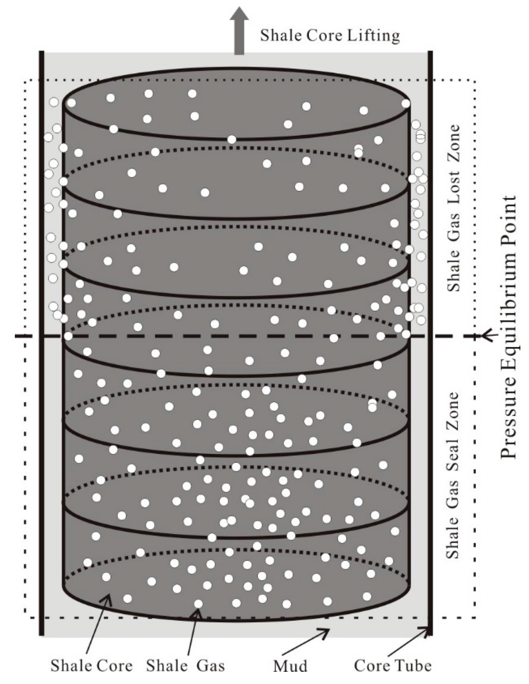
In order to identify the pressure equilibrium point quantitatively, we established a geological model of the lost shale gas during shale core lifting (Figure 4). On the basis of this model, we added several assumptions to the USBM method: (1) The initial drilling mud pressure is greater than the initial shale core pressure; (2) The point when the shale core pressure is the same as the drilling mud pressure is the true pressure equilibrium point for shale core. Above this point is the shale gas lost zone, and beneath this point is the shale gas seal zone; (3) Core lifting is a constant velocity process; (4) The gas dissolved in drilling mud is neglected. Based on these assumptions, we established Equations (6)–(8). Equation (9) could be derived from Equations (6)–(8). As shown in Equation (10), the total gas loss time (tloss) includes the gas loss time during core lifting (tequi) and the exposed ground time (texpo) before the core is loaded into the degassing canister. By bringing Equation (9) into Equation (10), the total gas loss time can be derived in Equation (11). By taking Equation (11) into Equation (5), Equation (12) can be derived. As the lost gas volume (vlost) is a negative value in Equation (12), the real lost gas volume (|vlost|) can be derived in Equation (13) by taking absolute value of the lost gas volume.
where tloss is the total gas loss time in minutes; tequi is the gas loss time during core lifting in minutes, which means the time from the pressure equilibrium point to the ground; texpo is the exposed ground time, from when shale is lifted to the ground to when shale is loaded into the degassing canisters; tdega is the cumulative degassing time during on-site shale degassing experiments in minutes; tlift is the core lifting time in minutes; hcore is the depth of core in meters; hequi is the depth of pressure equilibrium point in meters; F is the velocity of core lifting in m/s; ρwater is the density of water in kg/m3; ρmud is the density of drilling mud in kg/m3; k is the formation pressure coefficient; g is the acceleration of gravity, take 9.8 m/s2; vdega is the cumulative degassing shale gas volume in m3; vlost is a negative value of the lost gas volume in m3; |vlost| is the real lost gas volume in m3; and a is a constant.
We can use Equation (11), Equation (13) and Figure 5 to analyze the difference between the improved USBM method and the USBM method. When , (as shown in Equation (11)). The total gas loss time consists of two parts: one part is half of the core lifting time, and the other is the exposed ground time. Thus, it is very clear that the gas loss time from the improved USBM method is the same as the gas loss time from the USBM method, and the lost gas volumes by improved USBM method and by USBM method are the same as well. When , the total gas loss time from the improved USBM method is greater than the gas loss time from the USBM method, and the lost gas volume from the improved USBM method is greater than the lost gas volume by USBM method as well. When , the gas loss time from the improved USBM method is less than the gas loss time from the USBM method, and the lost gas volume from the improved USBM method is also less than the lost gas volume from the USBM method. Therefore, the gas loss time during core lifting is determined by the density of water (ρwater), the density of the drilling mud (ρmud) and the formation pressure coefficient (k).
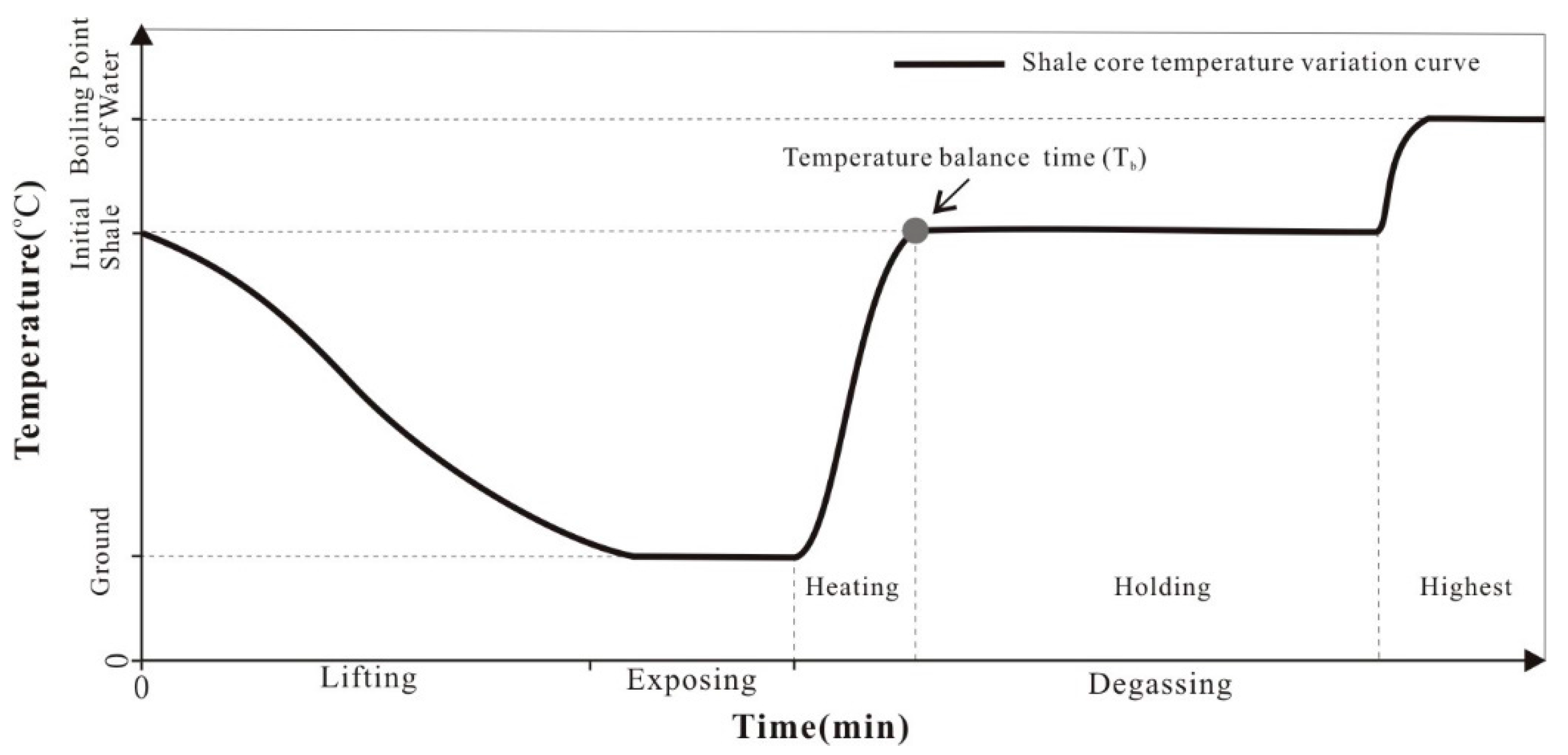
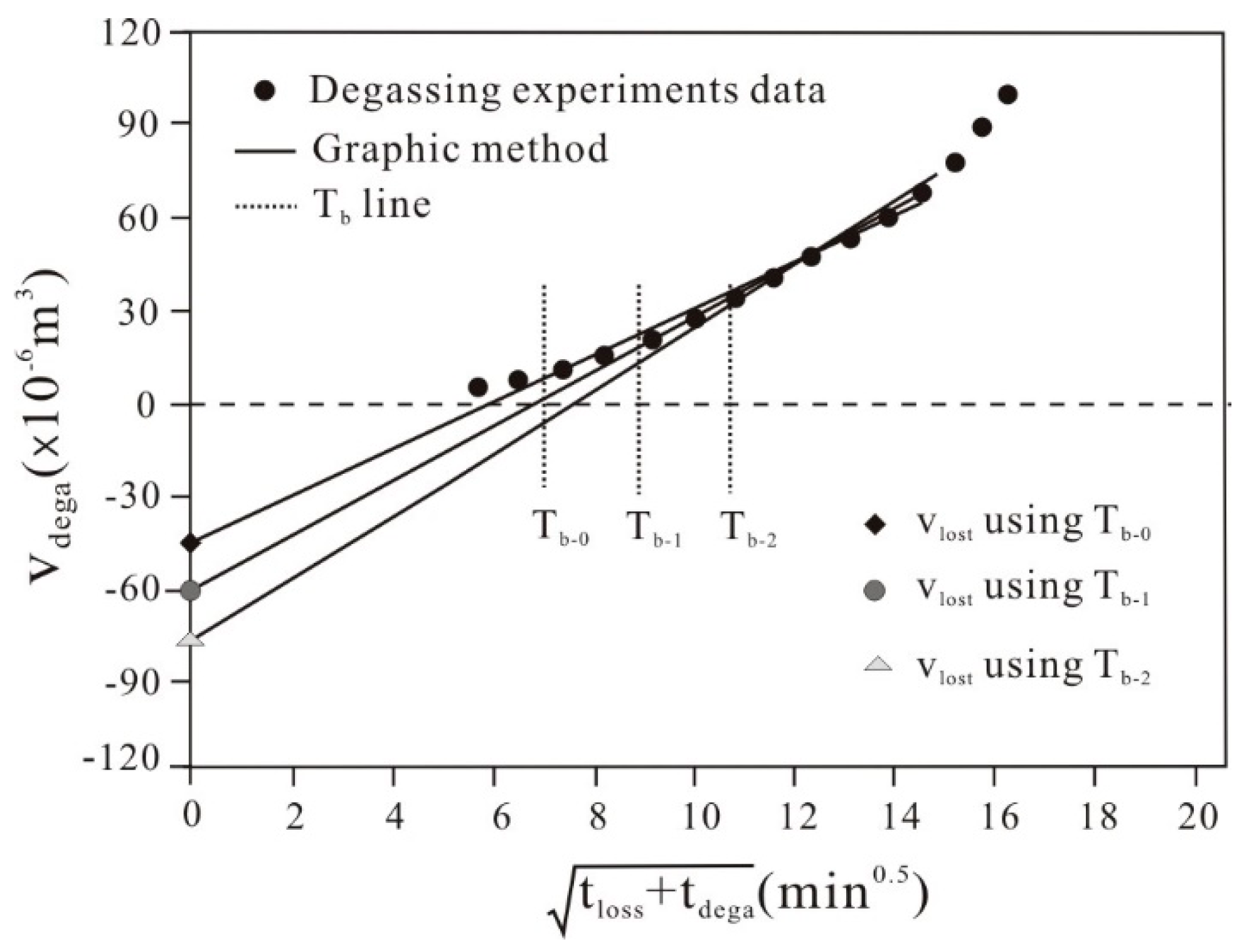
In order to determine the temperature balance time of water heating (Tb), the shale core temperature history was systematically analyzed in Figure 6. The initial shale core temperature was the reservoir temperature. The shale core temperature went down during shale core lifting and tended to a constant during shale core exposure. During on-site shale degassing experiments, the shale core temperature was heated to the reservoir temperature by water heating at first, held at the reservoir temperature; it eventually rose to the boiling point temperature of water. Holding the reservoir temperature is used to simulate the degassing process at the actual formation temperature. Raising the temperature to the boiling point makes the degassing process end fast. The temperature balance time (Tb) is the time when the shale core temperature was heated to the reservoir temperature. According to the USBM method, degassing experiment data before the temperature balance time could not reflect the actual degassing characteristic. Therefore, these data cannot be used to calculate the lost shale gas volume and should be abandoned [24,40]. An accurate temperature balance time is important for the calculation of lost shale gas volume. We illustrate it in Figure 7. Tb-0, Tb-1 and Tb-2 are three different temperature balance times, and Tb-2 is greater than Tb-1, while Tb-1 is greater than Tb-0. We can use some of the early degassing experiments’ data to calculate different lost gas volumes (Vlost) for Tb-0, Tb-1 and Tb-2 by a graphic method. As the degassing experiments’ data is on the slope-increasing process in the early degassing process, it is easy to see that Vlost of Tb-2 is greater than Vlost of Tb-1, and Vlost of Tb-1 is greater than Vlost of Tb-0. Assuming that Tb-1 is the real temperature balance time, using Tb-2 will make the Vlost too large and using Tb-0 will make the Vlost too small. Therefore, an accurate temperature balance time is very important for the calculation of lost shale gas volume.
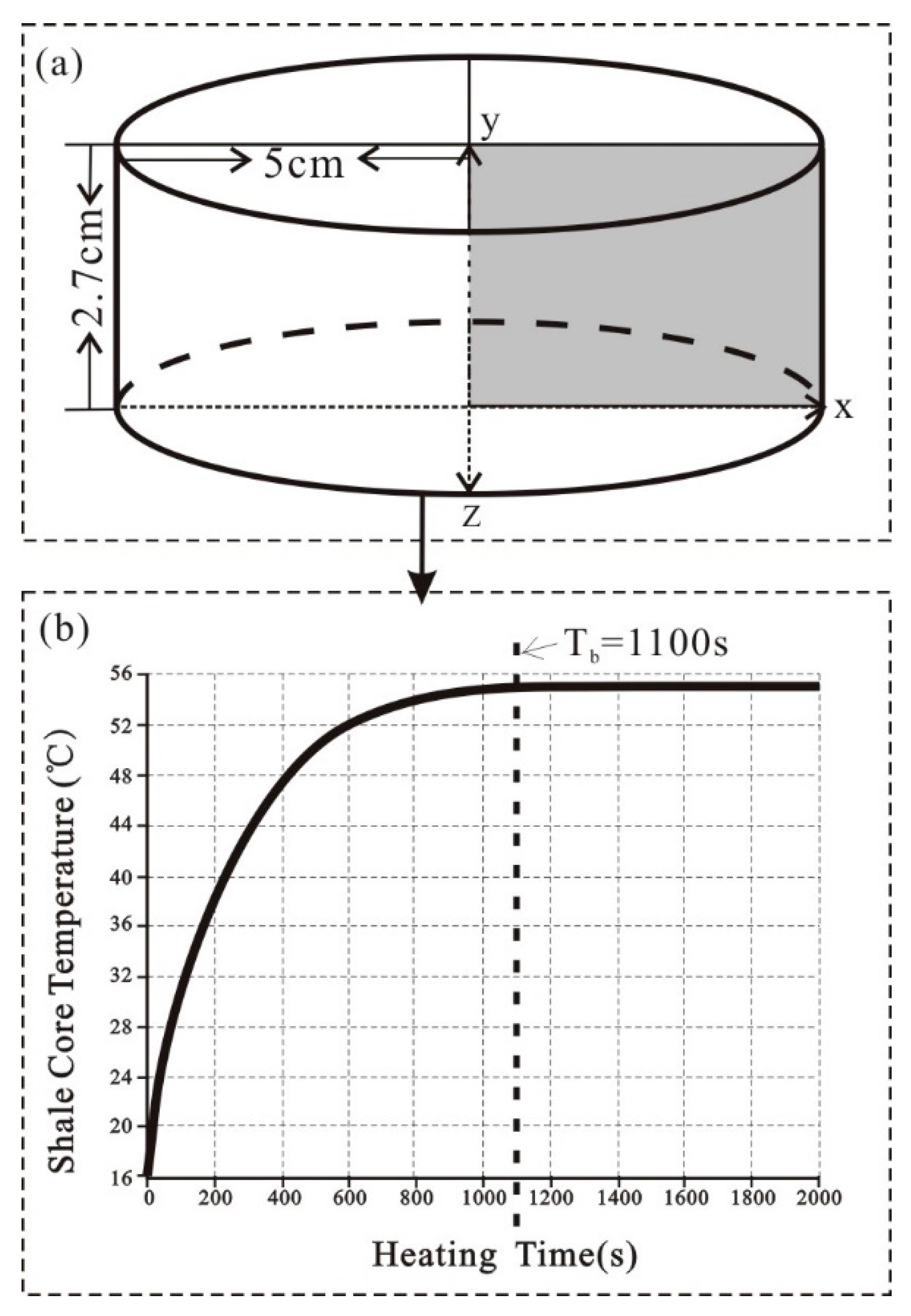
However, the USBM method uses human judgment to determine the temperature balance time and that may inevitably cause errors in calculating the lost shale gas volume. In order to avoid human errors, we use the finite element analysis method to obtain an accurate temperature balance time with the ANSYS software (ANSYS, Inc., Berkeley, CA, USA). The finite element analysis method is a numerical simulation method and we can use this method to analyze the thermal processes of heating (Figure 7). We can easily obtain an accurate temperature balance time using this method. The process of this method involves model building, loading, solving and post-processing. Take sample X1 as an example, a mathematical model of sample X1 was built at first as shown in Figure 8 (Figure 8a), the appropriate performance parameters of sample X1 were loaded and solved (Table 1). From the calculation results (Figure 8b), it is shown that the temperature of sample X1 reached the preset reservoir temperature (55 °C) at 1100 s. Therefore, 1100 s is the temperature balance time of sample X1.
3.2. Indirect Method
3.2.1. Adsorption Shale Gas Content
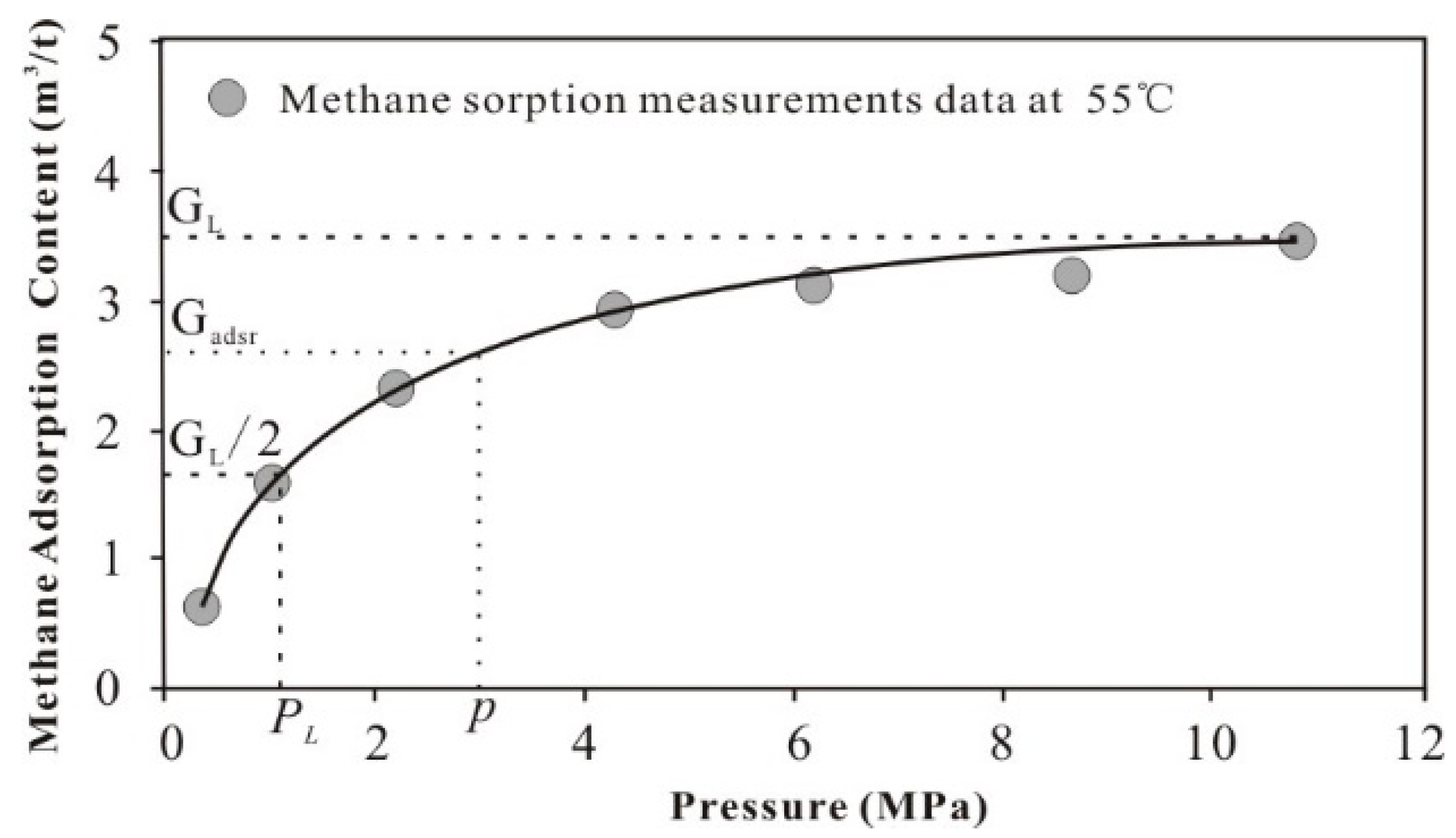
The total shale gas content of the indirect method is composed of three parts: adsorption shale gas content, free shale gas content and dissolved shale gas content (as shown in Equation (14)). Methane sorption measurements were conducted to obtain an accurate adsorption shale gas content. As shown in Figure 9, we determined the amount of adsorbed methane from minimum to maximum pressure at reservoir temperature at first, then the Langmuir model was used to calculate the Langmuir volume (GL) and the Langmuir pressure (PL). At last, the Langmuir volume (GL) and the Langmuir pressure (PL) could be used to calculate the adsorption shale gas content in Equation (15) [32,38,41,42,43].
where Gindirect is the total shale gas content of the indirect method in m3/t; Gadsr is the adsorption shale gas content in m3/t; Gfree is the free shale gas content in m3/t; Gdiss is the dissolved shale gas content in m3/t; GL is the Langmuir volume in m3/t, representing the maximum methane adsorption capacity of shale at a given temperature; PL is the Langmuir pressure in MPa, which is the pressure at half of the Langmuir volume; and p is the actual formation pressure of the shale reservoir in MPa.
3.2.2. Free Shale Gas Content
As shown in Equation (16), the free shale gas content is obtained by volume method [21,44].
where Gfree is the free shale gas content in m3/t, θ is the porosity of shale core obtained by logging technique method, Sg is pore gas saturation of shale core obtained by logging technique, ρ is the density of shale core in t/m3, and Bg is the volume factor.
3.2.3. Dissolved Shale Gas Content
The study of shale gas content mainly concentrates on the adsorption shale gas content and free shale gas content. There is little research on the dissolved shale gas content, which is considered unimportant and negligible. However, for some shale reservoirs with low maturity, the dissolved shale gas content takes up a large proportion and cannot be ignored. As shown in Equation (17), the dissolved shale gas content is divided into two parts: the water-dissolved shale gas content and oil-dissolved shale gas content. As shown in Equation (18), a new formula for calculating water dissolved shale gas content is derived by the volume method in this paper. The plate method proposed by Donson and Standing [45] is used to calculate the water-soluble gas solubility accurately. An accurate calculation of water-soluble gas solubility can makes the calculation of water-dissolved shale gas content accurate. As shown in Equation (19), a new formula for calculating oil-dissolved shale gas content is derived by the principle of similarity and dissolution in this paper. The residual hydrocarbon (S1) is used to indicate the residual oil in shale, and an empirical formula proposed by Vazquez and Beggs [46] is used to calculate the oil-soluble gas solubility. These make the calculation accuracy of dissolved shale gas content very high.
where Gdiss is the dissolved shale gas content in m3/t, Godiss is the oil dissolved shale gas content in m3/t, Gwdiss is the water dissolved shale gas content in m3/t, θ is the porosity of shale core obtained by logging technique method, Sw the is pore water saturation of shale core obtained by the logging technique, ρ is the density of the shale core in t/m3, ρo is the density of residual oil in t/m3, S1 is the residual hydrocarbon in mg/g, used to indicate the residual oil in shale, Rwdiss is the solubility of water-soluble gas in m3/m3, and Rodiss is the solubility of oil-soluble gas in m3/m3.
4. Results and Discussion
4.1. Direct Method
As shown in Table 2, the direct method above was used to calculate the shale gas content of 16 shale samples from the Triassic Yanchang Formation in the Southeastern Ordos Basin, China. The degassing shale gas content (Gdega) varies from 0.46 to 2.15 m3/t, with an average of 1.29 m3/t. The residual shale gas content (Gresi) varies from 0.08 to 0.59 m3/t, with an average of 0.24 m3/t. The lost shale gas content (Glost) varies from 1.30 to 3.91 m3/t, with an average of 2.44 m3/t. The total shale gas content from the direct method (Gdirect) is from 2.17 to 5.68 m3/t, with an average of 3.97 m3/t. A shale gas content greater than 2 m3/t can be used as an industrial development standard. Therefore, the shale gas content of the studied area is very large according to the improved USBM method.
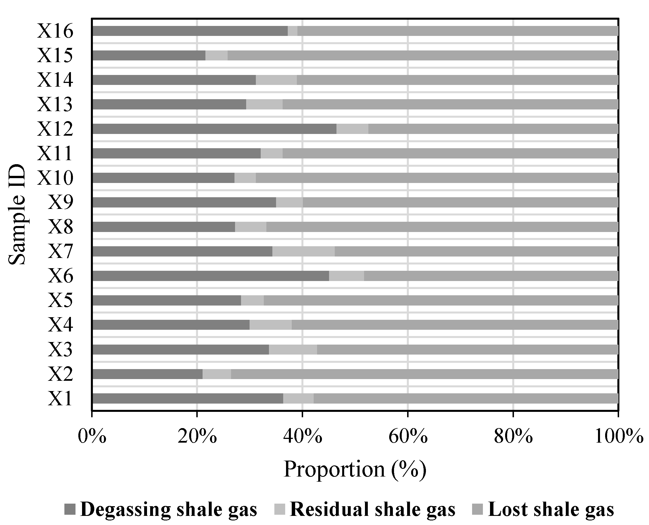
The proportion of degassing shale gas content, residual shale gas content and lost shale gas content was analyzed in Figure 10. The lost shale gas content is the largest proportion, with an average of 62%; the residual shale gas content is the smallest proportion, with an average of 6%; the average proportion of degassing shale gas content is 32%. Therefore, a large amount of shale gas is lost during shale core lifting and ground exposure.
As shown in Table 2, the results of the improved USBM method and the results of the USBM method were compared. Both the gas loss time (tloss) and the temperature balance time (Tb) determined by the improved USBM method were larger than those determined by the USBM method. Both the lost shale gas content (Glost) and the total shale gas content (Gdirect) determined by the improved USBM method were larger than those determined by the USBM method. Therefore, a large gas loss time and a large temperature balance time accounted for a large lost shale gas content.
4.2. Indirect Method
As shown in Table 3, the indirect method above was used to calculate the shale gas content of 16 shale samples from the Triassic Yanchang Formation in the Southeastern Ordos Basin, China. The adsorption shale gas content (Gadsr) ranges from 1.45 to 4.12 m3/t, with an average of 2.91 m3/t. The free shale gas content (Gfree) varies from 0.35 to 1.42 m3/t, with an average of 0.86 m3/t. The dissolved shale gas content (Gdiss) varies from 0.11 to 0.58 m3/t, with an average of 0.34 m3/t. The total shale gas content of indirect method (Gindirect) ranges from 1.91 to 6.02 m3/t, with an average of 4.11 m3/t. Therefore, the shale gas content of this area is very high according to the indirect method.
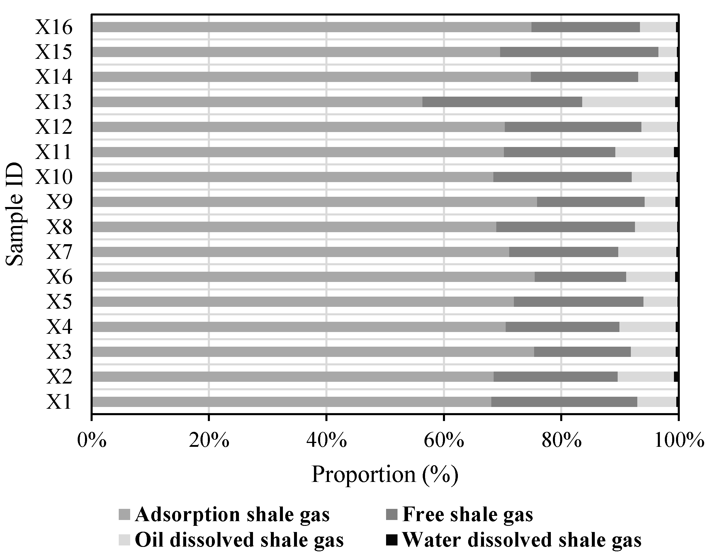
The proportion of adsorption shale gas content, free shale gas content and dissolved shale gas content are analyzed in Figure 11. The adsorption shale gas content is the largest proportion, with an average of 71%; the dissolved shale gas content is the smallest proportion, with an average of 8%; the average proportion of free shale gas content is 21%. Therefore, shale is mainly adsorption shale gas in the studied area. The dissolved shale gas content is mainly oil-dissolved shale gas content, which accounts for about 7.8%. Oil-dissolved shale gas may be caused by the low maturity of the shale reservoirs in this area. Therefore, attention should be paid to the oil-dissolved shale gas content and the water-dissolved shale gas content can be neglected in this area.
4.3. Comparison of Two Methods
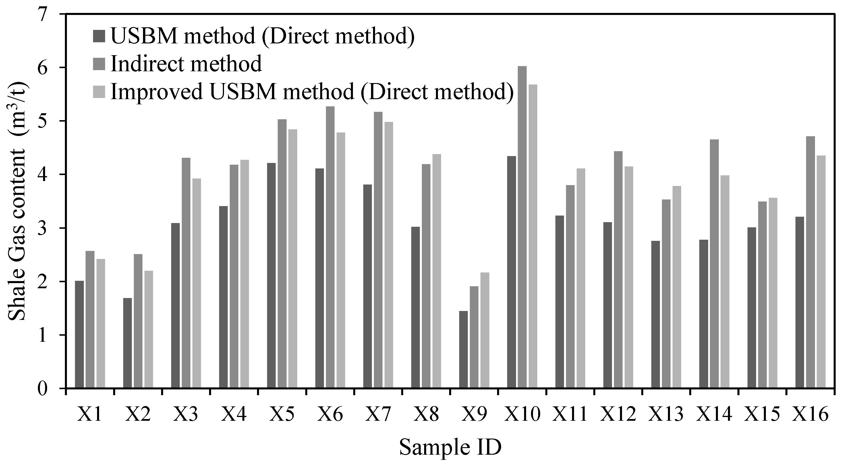
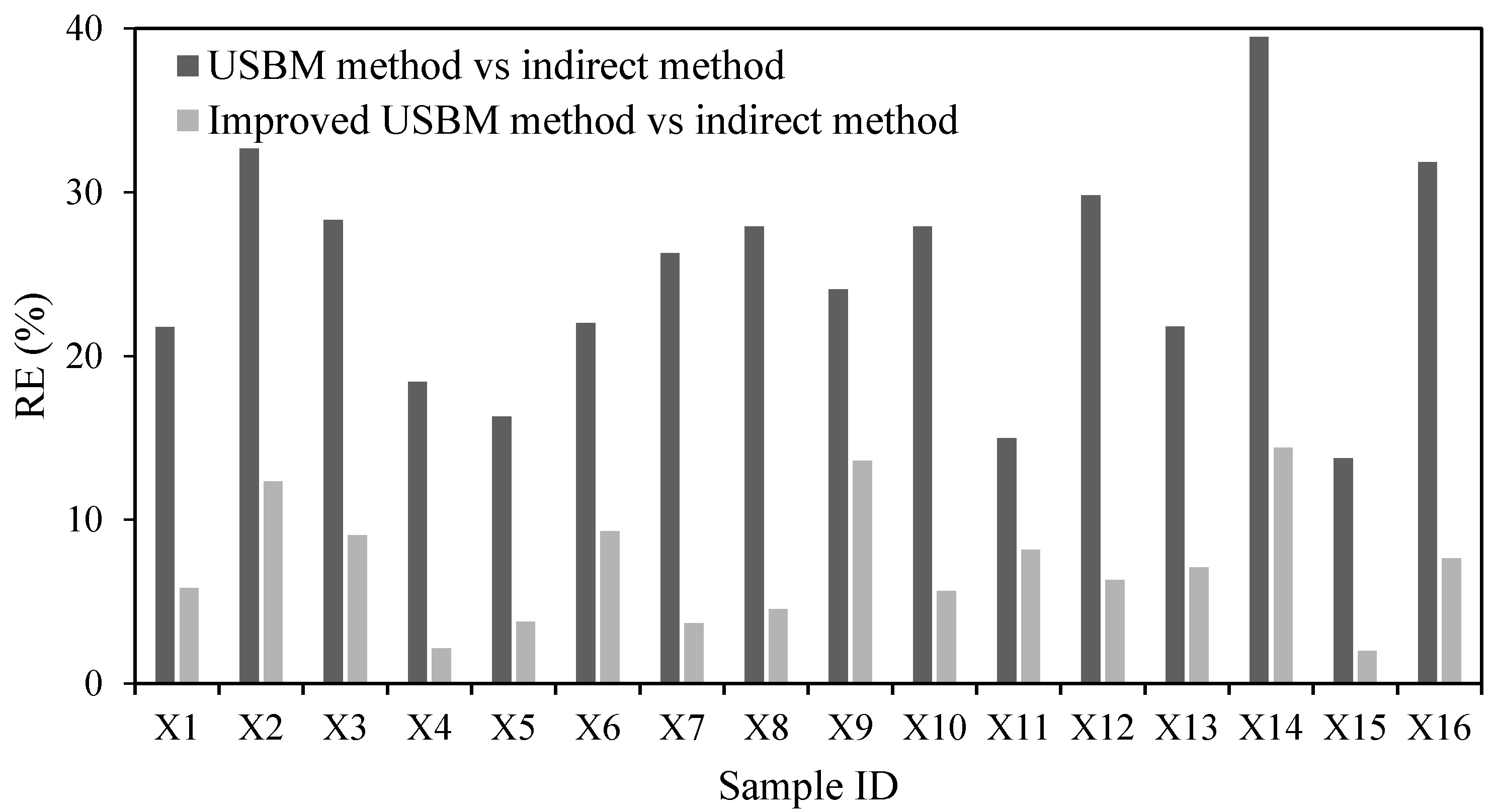
The direct method includes the USBM method and the improved USBM method. We compared the USBM method and the improved USBM method above, then we focused on the differences between the direct method and the indirect method. As shown in Figure 12, it is easy to see that the discrepancy between the improved USBM method and the indirect method is smaller than that between the USBM method and the indirect method. In order to quantitatively evaluate the differences between them, we analyzed their relative error (RE). The relative error of the USBM method vs. the indirect method (REUSBM) was evaluated by Equation (20). The relative error of the improved USBM method vs. the indirect method (REimproved) was evaluated by Equation (21). The results are shown in Figure 13. REUSBM is very large, with an average of about 24.8%. REimproved is very small, with an average of about 7.2%. It is clear that the discrepancy between the direct method and the indirect method is reduced by using the improved USBM method. The improved USBM method may be more practical and accurate than the USBM method.
where REUSBM is the relative error of the USBM method vs. the indirect method in %, REimproved is the relative error of the improved USBM method vs. the indirect method in %, GUSBM is the total shale gas content of the USBM method in m3/t, Gimproved is the total shale gas content of the improved USBM method in m3/t, and Gindirect is the total shale gas content of the indirect method in m3/t.
5. Conclusions
- (1)
- In order to make the USBM method more suitable for shale reservoirs, an improved USBM method is put forward. On the one hand, the shale core pressure history and drilling mud pressure history were systematically analyzed to identify the pressure equilibrium point and to determine the gas loss time quantitatively; on the other hand, the shale core temperature history was analyzed to obtain an accurate temperature balance time using the ANSYS software. The gas loss time during core lifting is determined by the density of water, the density of drilling mud and the formation pressure coefficient. The finite element analysis method allowed us to determine the temperature balance time accurately and avoid human error.
- (2)
- The direct method was used to calculate the shale gas content of 16 shale samples from the Triassic Yanchang Formation in the Southeastern Ordos Basin, China. The shale gas content of this area is very high according to the improved USBM method, with an average of 3.97 m3/t. The lost shale gas content is the largest proportion, with an average of 62%. Both the lost shale gas content and the total shale gas content determined by the improved USBM method are larger than those determined by the USBM method. In the studied area, a large gas loss time and a large temperature balance time make a large lost shale gas content.
- (3)
- The indirect method was used to calculate the shale gas content of 16 shale samples from the Triassic Yanchang Formation in the Southeastern Ordos Basin, China. The shale gas content of this area is very high according to the indirect method, with an average of 4.11 m3/t. The adsorption shale gas content is the largest proportion, with an average of 71%. The dissolved shale gas content is mainly the oil-dissolved shale gas content, which accounts for about 7.8%. Attention should be paid to the oil-dissolved shale gas content and the water-dissolved shale gas content can be neglected in the studied area.
- (4)
- The shale gas content of the direct method and the indirect method were compared. The discrepancy between the direct method and the indirect method is reduced by using the improved USBM method, and the improved USBM method could be more practical and accurate than the USBM method.
Author Contributions
Jiao Su and Jin Hao conceived and designed the experiments; Jin Hao performed the experiments; Jiao Su and Yingchun Shen analyzed the data; Bo Liu contributed the reagents and testing materials; Jiao Su and Yingchun Shen wrote the paper, and Jiao Su, Yingchun Shen, Jin Hao were responsible for the final proofreading of the article.
Conflicts of Interest
The authors declare no conflict of interest.
References
- Mavor, M. ABSTRACT: Barnett Shale Gas-in-Place Volume including Sorbed and Free Gas Volume; Fort Worth Geological Society: Houston, TX, USA, 2003. [Google Scholar]
- Jarvie, D.M.; Hill, R.J.; Ruble, T.E.; Pollastro, R.M. Unconventional shale-gas systems: The Mississippian Barnett Shale of north-central Texas as one model for thermogenic shale-gas assessment. AAPG Bull. 2007, 91, 475–499. [Google Scholar] [CrossRef]
- Brittenham, M.D. Geologic analysis of the Upper Jurassic Haynesville Shale in east Texas and west Louisiana: Discussion. AAPG Bull. 2013, 97, 525–528. [Google Scholar] [CrossRef]
- Zhang, J.C.; Xu, B.; Nie, H.K.; Wang, Z.Y.; Lin, T. Exploration potential of shale gas resources in China. Nat. Gas Ind. 2008, 28, 136–140. [Google Scholar]
- Dong, D.Z.; Zou, C.N.; Li, J.Z.; Wang, S.J.; Li, X.J.; Wang, Y.M.; Li, D.H.; Huang, J.L. Resource potential, exploration and development prospect of shale gas in the whole world. Geol. Bull. China 2011, 31, 324–336. [Google Scholar]
- Zhou, C.N.; Dong, D.Z.; Wang, S.J.; Li, J.Z.; Li, X.J.; Wang, Y.M.; Li, D.H.; Cheng, K.M. Geological characteristics characteristics, formation mechanism and resource potential of shale gas in China. Pet. Explor. Dev. 2010, 37, 641–653. [Google Scholar] [CrossRef]
- Yang, Y.T.; Zhang, J.C.; Wang, X.Z.; Cao, J.Z.; Tang, X.; Wang, L.; Yang, S.Y. Source rock evaluation of continental shale gas: A case study of Chang 7 of Mesozoic Yangchang Formation in Xia Siwan area of Yanchang. J. Northeast Pet. Univ. 2012, 36, 10–17. [Google Scholar]
- Wang, Z.G. Breakthrough of Fuling shale gas exploration and development and its inspiration. Oil Gas Geol. 2015, 36, 1–6. [Google Scholar]
- Wu, Q.; Liang, X.; Xian, C.G.; Li, X. Geoscience-to-production integration ensures effective and efficient south China marine shale gas development. China Pet. Explor. 2015, 20, 1–23. [Google Scholar]
- Guo, X.S. Rules of Two-Factor enrichment for marine shale gas in southern China: Understanding from the Longmaxi formation shale gas in Sichuan basin and its surrounding area. Acta Geol. Sin. 2014, 8, 1209–1218. [Google Scholar]
- Guo, T.L.; Zhang, H.R. Formation and enrichment mode of Jiaoshiba shale gas field, Sichuan Basin. Pet. Explor. Dev. 2014, 41, 28–36. [Google Scholar] [CrossRef]
- Zhang, D. Future Development Trend of China’s Unconventional Oil and Gas Resources and Shale Gas. Land Resour. Inf. 2016, 11, 3–7. [Google Scholar]
- Zou, C.; Zhao, Q.; Zhang, G.S.; Xiong, B. Energy revolution: From a fossil energy era to a new energy era. Nat. Gas Ind. B 2016, 3, 1–11. [Google Scholar] [CrossRef]
- Jia, C. Breakthrough and significance of unconventional oil and gas to classical petroleum geological theory. Pet. Explor. Dev. 2017, 44, 1–11. [Google Scholar] [CrossRef]
- Montgomery, S.L.; Jarvie, D.M.; Bowker, K.A.; Pollastro, R.M. Mississippian Barnett Shale, Fort Worth basin, north-central Texas: Gas-shale play with multi-trillion cubic foot potential. AAPG Bull. 2005, 89, 155–175. [Google Scholar] [CrossRef]
- Bowker, K.A. Barnett shale gas production, Fort Worth Basin: Issues and discussion. AAPG Bull. 2007, 91, 523–533. [Google Scholar] [CrossRef]
- Ross, D.J.K.; Bustin, R.M. Characterizing the shale gas resource potential of Devonian—Mississippian strata in the Western Canada sedimentary basin: Application of an integrated formation evaluation. AAPG Bull. 2008, 92, 87–125. [Google Scholar] [CrossRef]
- Curtis, J.B. Fractured shale-gas systems. AAPG Bull. 2002, 86, 1921–1938. [Google Scholar]
- Li, Y.X.; Qiao, D.W.; Jiang, W.L.; Zhang, C.H. Gas content of gas-bearing shale and its geological evaluation summary. Geol. Bull. China 2011, 30, 308–317. [Google Scholar]
- Zeng, W.; Zhang, J.; Ding, W.; Wang, X.; Zhu, D.; LIU, Z. The gas content of continental Yanchang shale and its main controlling factors: A case study of Liuping-171 well in Ordos Basin. Nat. Gas Geosci. 2014, 25, 291–301. [Google Scholar]
- Dong, Q.; Liu, X.P.; Li, W.G.; D, Q.Y. Determination of gas content in shale. Nat. Gas Oil 2012, 30, 34–37. [Google Scholar]
- Tang, Y.; Zhang, J.C.; Li, L.Z. Use and improvement of the desorption method in shale gas content tests. Nat. Gas Ind. 2011, 31, 108–112. [Google Scholar]
- Wilson, K.; Padmakar, A.S.; Mondegarian, F. Simulation of core lifting process for lost gas calculation in shale reservoirs. In Proceedings of the International Symposium of the Society of Core Analysts, Napa Valley, CA, USA, 16–19 September 2013; SCA: Milpitas, CA, USA, 2013. [Google Scholar]
- Kissell, F.N.; Mcculloch, C.M.; Elder, C.H. The Direct Method of Determining Methane Content of Coal Beds for Ventilation Design; Technical Report; Pittsburgh Mining and Safety Research Center: Pittsburgh, PA, USA, 1973. [Google Scholar]
- Smith, D.M.; Williams, F.L. New technique for determining the methane content of coal. In Proceedings of the 16th Intersociety Energy Conversion Engineering Conference, Atlanta, GA, USA, 9–14 August 1981; ASME: New York, NY, USA, 1981. [Google Scholar]
- Smith, D.M.; Williams, F.L. Diffusion models for gas production from coal: Determination of diffusion parameters. Fuel 1984, 63, 256–261. [Google Scholar] [CrossRef]
- Dan, Y.; Seidle, J.P.; Hanson, W.B. Gas Sorption on Coal and Measurement of Gas Content. In SG 38: Hydrocarbons from Coal; El discurso civilizador en Derecho Internacional; Cinco estudios y tres comentarios; Instituto Fernando el Católico (IFC): Zaragoza, Spain, 1993; pp. 203–218. [Google Scholar]
- Zhang, J.; Xue, H.; Zhang, D. Shale gas and its accumulation mechanism. Geoscience 2003, 17, 466. [Google Scholar]
- Lewis, R.; Ingraham, D.; Pearcy, M.; Williamson, J.; Sawyer, W.; Frantz, J. New evaluation techniques for gas shale reservoirs. In Reservoir Symposium; Schlumberger: Houston, TX, USA, 2004. [Google Scholar]
- Hao, J.F.; Zhou, C.C.; Li, X.; Cheng, X.Z.; Song, L.T. Summary of shale gas evaluation applying geophysical logging. Prog. Geophys. 2012, 27, 1624–1632. [Google Scholar]
- Zhong, G.H.; Xie, B.; Zhou, X.; Peng, X.; Tian, C. A logging evaluation method for gas content of shale gas reservoirs in the Sichuan Basin. Nat. Gas Ind. 2016, 36, 43–51. [Google Scholar]
- Li, W.G.; Yang, S.L.; Xu, J.; D, Q. A new model for shale adsorptive gas amount under a certain geological conditions of temperature and pressure. Nat. Gas Geosci. 2012, 23, 791–796. [Google Scholar]
- Zhang, Q.; Liu, H.I.; Bai, W.H.; Lin, W. Shale gas content and its main controlling factors in Longmaxi shale in southeastern Chongqing. Nat. Gas Ind. 2013, 33, 35–39. [Google Scholar]
- Lau, H.C.; Li, H.; Huang, S. Challenges and Opportunities of Coalbed Methane Development in China. Energy Fuels 2017, 31, 4588–4602. [Google Scholar] [CrossRef]
- Li, H.; Lau, H.C.; Huang, S. Coalbed Methane Development in China: Engineering Challenges and Opportunities. In Proceedings of the SPE/IATMI Asia Pacific Oil & Gas Conference and Exhibition, Jakarta, Indonesia, 17–19 October 2017. [Google Scholar]
- Meng, Z.; Liu, C.; Ji, Y. Geological conditions of coalbed methane and shale gas exploitation and their comparison analysis. J. China Coal Soc. 2013, 38, 728–736. [Google Scholar]
- GB/T 19560-2008. Experimental Method of High-Pressure Isothermal Adsorption to Coal; Standardization Administration of the People’s Republic of China: Beijing, China, 2008. [Google Scholar]
- Langmuir, I. The adsorption of gases on plane surfaces of glass, mica and platinum. J. Chem. Phys. 1918, 40, 1361–1403. [Google Scholar] [CrossRef]
- Jiang, Y.L.; Xue, H.Q.; Wang, H.Y.; Liu, H.L.; Yan, G. The Measurement of Shale Gas Content. Appl. Mech. Mater. 2013, 288, 333–337. [Google Scholar] [CrossRef]
- Liu, H.L.; Deng, Z.; Liu, D.X.; Zhao, Q.; Kang, Y.S.; Zhao, H.X. Discussion on lost gas calculating methods in shale gas content testing. Oil Drill. Prod. Technol. 2010, 322, 156–158. [Google Scholar]
- Gregg, S.J.; Sing, K.S.W. Adsorption, Surface Area, and Porosity; Academic Press: Cambridge, MA, USA, 1982. [Google Scholar]
- Bandosz, T.J. Gas Adsorption EquiIibria: Experimental Methods and Adsorptive Isotherms. J. Am. Chem. Soc. 2005, 127, 7655–7656. [Google Scholar] [CrossRef]
- Wang, F.Y.; He, Z.Y.; Meng, X.H.; Bao, L.Y.; Zhang, H. Occurrence of Shale Gas and Prediction of Original Gas In-place (OGIP). Nat. Gas Geosci. 2011, 22, 501–510. [Google Scholar]
- Li, Y. Calculation Methods of Shale Gas Reserves. Nat. Gas Geosci. 2009, 20, 466–470. [Google Scholar]
- Dodson, C.R.; Standing, M.B. Pressure-volume-temperature and solubility relations for natural-gas-water mixtures. In Drilling and Production Practice; American Petroleum Institute: Washington, DC, USA, 1944. [Google Scholar]
- Vazquez, M.; Beggs, H.D. Correlations for fluid physical property prediction. J. Pet. Technol. 1980, 32, 968–970. [Google Scholar] [CrossRef]
Figure 1.
Composition of water heating degassing instrument.

Figure 2.
The determination of lost gas volume using a graphic method of the USBM.
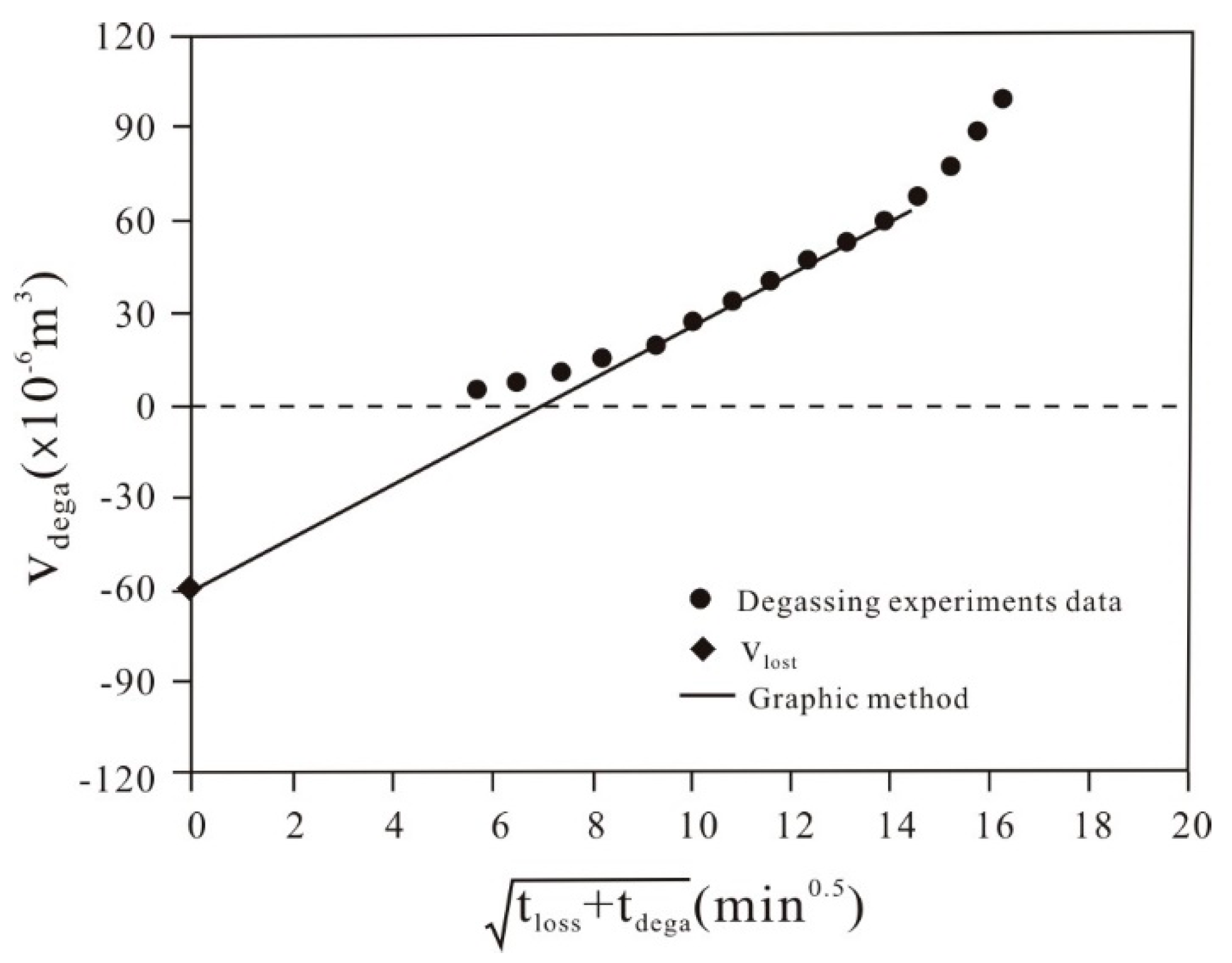
Figure 3.
A systematic analysis of pressure history.
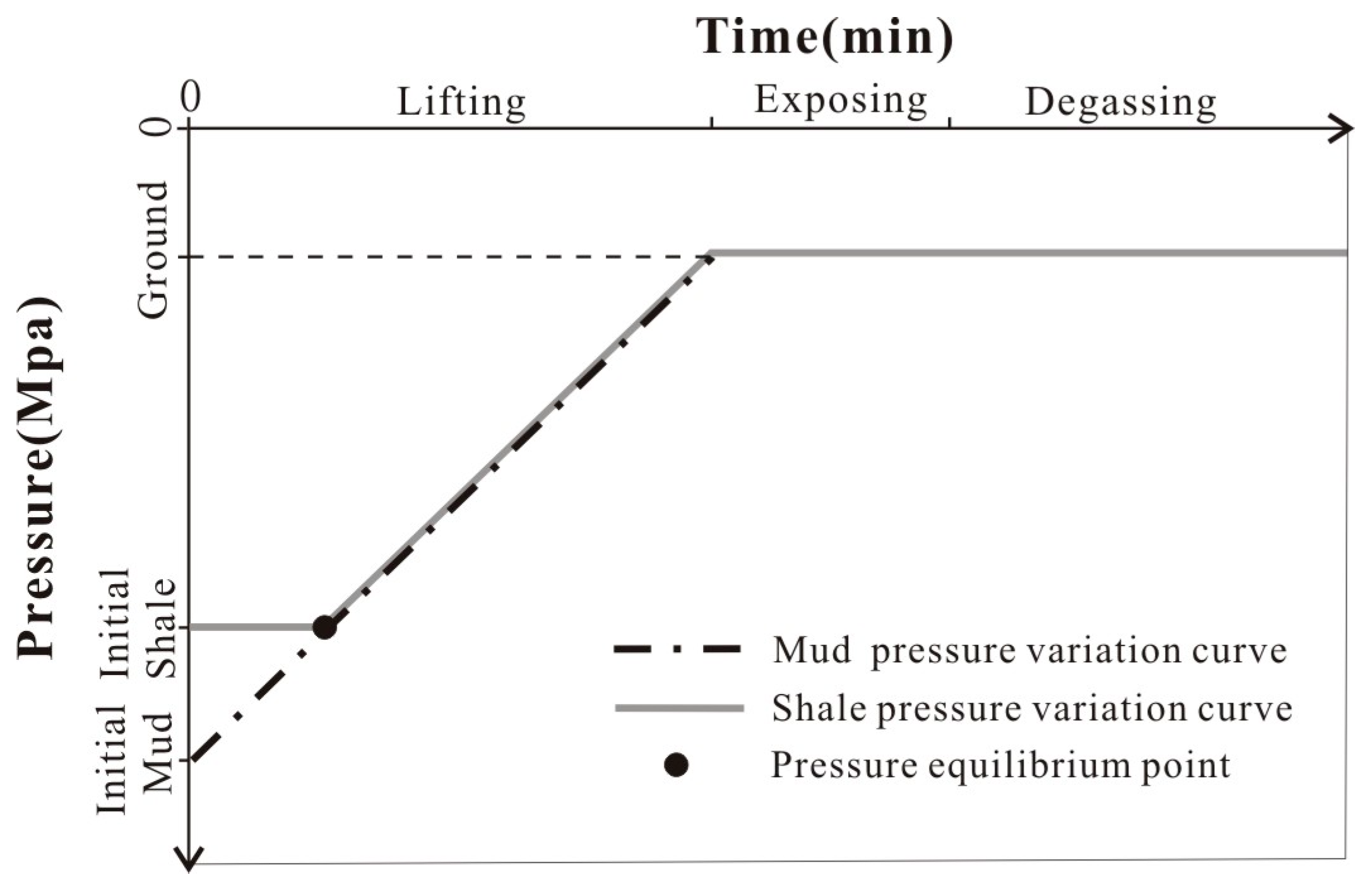
Figure 4.
A geological model of the lost shale gas during shale core lifting.

Figure 5.
The calculation of lost gas volume in three types of gas loss time.
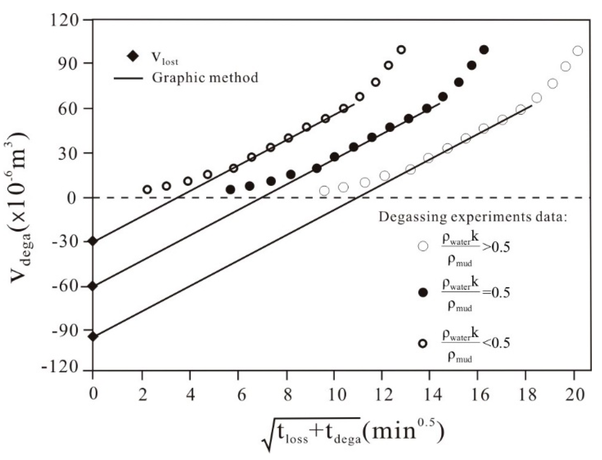
Figure 6.
The temperature history of shale core.

Figure 7.
The calculation of lost gas volume in three types of temperature balance time.

Figure 8.
The process of calculating the temperature balance time of sample X1 using ANSYS software. (a) Mathematical model; (b) Calculation results.
Figure 8.
The process of calculating the temperature balance time of sample X1 using ANSYS software. (a) Mathematical model; (b) Calculation results.

Figure 9.
The calculation of adsorption shale gas content by the Langmuir model.

Figure 10.
The proportion of degassing shale gas content, residual shale gas content and lost shale gas content.
Figure 10.
The proportion of degassing shale gas content, residual shale gas content and lost shale gas content.

Figure 11.
The proportion of adsorption shale gas content, residual shale gas content and lost shale gas content.
Figure 11.
The proportion of adsorption shale gas content, residual shale gas content and lost shale gas content.

Figure 12.
A comparison of shale gas content between the USBM method, the improved USBM method and the indirect method.
Figure 12.
A comparison of shale gas content between the USBM method, the improved USBM method and the indirect method.

Figure 13.
The results of relative error (RE).


Table 1.
The performance parameters of sample X1.
| Parameter | Value | Parameter | Value |
|---|---|---|---|
| Radius | 5 cm | Surface heat coefficient | 15 W/(m2·°C) |
| Thickness | 2.7 cm | Specific heat capacity | 876 J/kg·°C |
| Initial temperature | 15 °C | Density | 2430 kg/m3 |
| Water heating temperature | 55 °C | Thermal conductivity | 5 W/(m·°C) |
Table 2.
The results of shale gas content by the direct method.
| Sample ID | Depth (m) | Gdesr (m3/t) | Gresi (m3/t) | Calculating Glost | Gdirect (m3/t) | ||||||
|---|---|---|---|---|---|---|---|---|---|---|---|
| tloss (min) | Tb (min)a | Glost (m3/t) | |||||||||
| USBM | Improved | USBM | Improved | USBM | Improved | USBM | Improved | ||||
| X1 | 1336.72 | 0.88 | 0.14 | 177 | 217 | 12 | 18 | 0.99 | 1.40 | 2.01 | 2.42 |
| X2 | 1409.04 | 0.46 | 0.12 | 262 | 321 | 14 | 23 | 1.11 | 1.62 | 1.69 | 2.20 |
| X3 | 1419.83 | 1.32 | 0.36 | 342 | 401 | 8 | 20 | 1.41 | 2.24 | 3.09 | 3.92 |
| X4 | 1392.11 | 1.28 | 0.34 | 227 | 281 | 12 | 22 | 1.79 | 2.65 | 3.41 | 4.27 |
| X5 | 1390.25 | 1.37 | 0.21 | 240 | 297 | 10 | 16 | 2.63 | 3.26 | 4.21 | 4.84 |
| X6 | 1400.71 | 2.15 | 0.32 | 188 | 227 | 14 | 20 | 1.64 | 2.31 | 4.11 | 4.78 |
| X7 | 1338.48 | 1.71 | 0.59 | 264 | 300 | 10 | 19 | 1.51 | 2.68 | 3.81 | 4.98 |
| X8 | 1346.75 | 1.19 | 0.26 | 183 | 223 | 9 | 21 | 1.57 | 2.93 | 3.02 | 4.38 |
| X9 | 1456.31 | 0.76 | 0.11 | 231 | 301 | 11 | 20 | 0.58 | 1.30 | 1.45 | 2.17 |
| X10 | 1387.61 | 1.54 | 0.23 | 198 | 253 | 12 | 21 | 2.57 | 3.91 | 4.34 | 5.68 |
| X11 | 1466.87 | 1.32 | 0.17 | 212 | 307 | 7 | 18 | 1.74 | 2.62 | 3.23 | 4.11 |
| X12 | 1478.24 | 1.93 | 0.25 | 277 | 354 | 8 | 17 | 0.93 | 1.97 | 3.11 | 4.15 |
| X13 | 1354.12 | 1.11 | 0.26 | 241 | 321 | 14 | 23 | 1.39 | 2.41 | 2.76 | 3.78 |
| X14 | 1423.27 | 1.24 | 0.31 | 331 | 412 | 12 | 22 | 1.23 | 2.43 | 2.78 | 3.98 |
| X15 | 1321.34 | 0.77 | 0.15 | 245 | 332 | 8 | 17 | 2.09 | 2.64 | 3.01 | 3.56 |
| X16 | 1378.23 | 1.62 | 0.08 | 168 | 243 | 13 | 24 | 1.51 | 2.65 | 3.21 | 4.35 |
Table 3.
The results of shale gas content by the indirect method.
| Sample ID | Depth (m) | Gadsr (m3/t) | Gfree (m3/t) | Dissolved Gas Content | Gindirect (m3/t) | ||
|---|---|---|---|---|---|---|---|
| Godiss (m3/t) | Gwdiss (m3/t) | Gdiss (m3/t) | |||||
| X1 | 1336.72 | 1.75 | 0.64 | 0.17 | 0.01 | 0.18 | 2.57 |
| X2 | 1409.04 | 1.72 | 0.53 | 0.24 | 0.02 | 0.26 | 2.51 |
| X3 | 1419.83 | 3.25 | 0.71 | 0.33 | 0.02 | 0.35 | 4.31 |
| X4 | 1392.11 | 2.95 | 0.81 | 0.40 | 0.02 | 0.42 | 4.18 |
| X5 | 1390.25 | 3.62 | 1.11 | 0.29 | 0.01 | 0.30 | 5.03 |
| X6 | 1400.71 | 3.98 | 0.82 | 0.44 | 0.03 | 0.47 | 5.27 |
| X7 | 1338.48 | 3.68 | 0.96 | 0.51 | 0.02 | 0.53 | 5.17 |
| X8 | 1346.75 | 2.89 | 0.99 | 0.30 | 0.01 | 0.31 | 4.19 |
| X9 | 1456.31 | 1.45 | 0.35 | 0.10 | 0.01 | 0.11 | 1.91 |
| X10 | 1387.61 | 4.12 | 1.42 | 0.46 | 0.02 | 0.48 | 6.02 |
| X11 | 1466.87 | 2.67 | 0.72 | 0.38 | 0.03 | 0.41 | 3.80 |
| X12 | 1478.24 | 3.12 | 1.03 | 0.27 | 0.01 | 0.28 | 4.43 |
| X13 | 1354.12 | 1.99 | 0.96 | 0.56 | 0.02 | 0.58 | 3.53 |
| X14 | 1423.27 | 3.48 | 0.85 | 0.29 | 0.03 | 0.32 | 4.65 |
| X15 | 1321.34 | 2.43 | 0.94 | 0.11 | 0.01 | 0.12 | 3.49 |
| X16 | 1378.23 | 3.53 | 0.87 | 0.29 | 0.02 | 0.31 | 4.71 |
© 2017 by the authors. Licensee MDPI, Basel, Switzerland. This article is an open access article distributed under the terms and conditions of the Creative Commons Attribution (CC BY) license (http://creativecommons.org/licenses/by/4.0/).
Share and Cite
MDPI and ACS Style
Su, J.; Shen, Y.; Hao, J.; Liu, B. Shale Gas Content Calculation of the Triassic Yanchang Formation in the Southeastern Ordos Basin, China. Energies 2017, 10, 1949. https://doi.org/10.3390/en10121949
AMA Style
Su J, Shen Y, Hao J, Liu B. Shale Gas Content Calculation of the Triassic Yanchang Formation in the Southeastern Ordos Basin, China. Energies. 2017; 10(12):1949. https://doi.org/10.3390/en10121949
Chicago/Turabian StyleSu, Jiao, Yingchu Shen, Jin Hao, and Bo Liu. 2017. "Shale Gas Content Calculation of the Triassic Yanchang Formation in the Southeastern Ordos Basin, China" Energies 10, no. 12: 1949. https://doi.org/10.3390/en10121949
Note that from the first issue of 2016, this journal uses article numbers instead of page numbers. See further details here.