Energy Management and Control of Plug-In Hybrid Electric Vehicle Charging Stations in a Grid-Connected Hybrid Power System

Abstract

The charging infrastructure plays a key role in the healthy and rapid development of the electric vehicle industry. This paper presents an energy management and control system of an electric vehicle charging station. The charging station (CS) is integrated to a grid-connected hybrid power system having a wind turbine maximum power point tracking (MPPT) controlled subsystem, photovoltaic (PV) MPPT controlled subsystem and a controlled solid oxide fuel cell with electrolyzer subsystem which are characterized as renewable energy sources. In this article, an energy management system is designed for charging and discharging of five different plug-in hybrid electric vehicles (PHEVs) simultaneously to fulfil the grid-to-vehicle (G2V), vehicle-to-grid (V2G), grid-to-battery storage system (G2BSS), battery storage system-to-grid (BSS2G), battery storage system-to-vehicle (BSS2V), vehicle-to-battery storage system (V2BSS) and vehicle-to-vehicle (V2V) charging and discharging requirements of the charging station. A simulation test-bed in Matlab/Simulink is developed to evaluate and control adaptively the AC-DC-AC converter of non-renewable energy source, DC-DC converters of the storage system, DC-AC grid side inverter and the converters of the CS using adaptive proportional-integral-derivate (AdapPID) control paradigm. The effectiveness of the AdapPID control strategy is validated through simulation results by comparing with conventional PID control scheme.

1. Introduction

In the world today, fossil fuels are the dominant energy sources for power generation, but the depletion of fossil fuel reserves along with growing environmental concerns have been a wake-up call for finding the alternative energy sources. In the past few decades, the integration of renewable energy sources (RES) along with energy storage systems has been gaining a remarkable pace throughout the world. Plug-in hybrid electric vehicles (PHEVs) are achieving great popularity owing to the global call for clean energy [1]. The penetration of PHEVs in the power grid constitutes an emerging technology [2,3].

The RES and PHEVs potentially not only provide a clean and environmentally friendly, but also cost-effective energy. Among RES, the wind and photovoltaic (PV) power are considered foremost energy sources, because they are abundantly available in Nature [4,5]. The inherent issue of RES is their intermittent nature, therefore, the utilization of RES needs to incorporate energy storage systems [6]. Solid oxide fuel cells (SOFCs) are used as an alternative and versatile energy source [7]. SOFCs provide fuel flexibility, high efficiency and low emissions. The PHEV charging station (CS) integrated into a grid-connected hybrid power system (HPS) offers a bidirectional power flow between the utility grid and the CS [8,9]. The bidirectional power flow between utility grid and CS improves the HPS reliability [10]. However, the energy management and appropriate control for PHEVs charging station integrated into a grid-connected HPS are the potential areas of concern [11,12].

In a CS, the process of charging an uncertain number of PHEVs with varying energy demand causes a demand side management dilemma. Ultimately, the peak demand will be driven up which may cause system instability. An effective energy management strategy (EMS) controls the load peak [13,14]. In the literature, the main approaches reported for EMS are dynamic programming (DP) [15], predictive framework [16], meta-heuristic algorithms [17,18] and neural networks (NNs) [19,20]. The DP computes the global optimal solution, but the computational complexity increases rapidly with the number of states and control variables. The predictive EMS integrates the real-time traffic flow velocity data. It quickly generates a state-of-charge (SOC) trajectory for a PHEV to avoid a particular traffic route. However, the predictive framework is computationally complex and unable to deal with the uncertainties. Meta-heuristic algorithms do not involve derivative-based calculations and converge to a global optimum. However, these algorithms have long computation times, because an acceptable accuracy is achieved only after a large number of iterations. NNs are fast computing, easy to implement and intelligent decision makers, yet the accuracy of NNs depends upon the amount and quality of training.

PHEVs are considered a stochastic controllable load. The random nature of PHEVs’ load has an unfavorable influence on the HPS reliability. The deterioration of HPS reliability affects the frequency regulation, spinning reserves and load voltage profile [21]. Therefore, an appropriate PHEV charging/discharging control strategy is necessary to improve the HPS reliability. There are two types of PHEVs charging techniques, i.e., uncoordinated or coordinated [22]. In uncoordinated charging, only unidirectional power flow takes place. The PHEVs are directly charged from the grid until their maximum SOC limit. However, uncoordinated charging increases the load at peak demand hours which leads to grid instability and power quality issues. The coordinated charging is characterized by bidirectional power flow which is used for charging of PHEVs and providing supplementary power back to the grid. The coordinated charging approach offers a number of advantages which include reduction in peak demand [23], minimization of the HPS operational cost [24], improvement of frequency regulation [25] and increase in the HPS reliability [26].

In the literature, numerous conventional techniques are used to control charging/discharging of PHEVs in a HPS. These conventional techniques involve quadratic programming and dynamic programming [27], mixed integer programming [24], linear programming [28] and proportional-integral (PI) control [29]. However, these conventional control systems are designed for a certain operating state and are not capable to adopt to a fluctuating environment. In case of large excursions, the system variables may go out of bound and result in system instability. Adaptive control is magnificently used to solve nonlinear and time varying uncertain control problems. Adaptive control is preferred over conventional control, because adaptive control is capable of online dealing with system nonlinearities, uncertainties and variations. A hybrid particle swarm optimization-based adaptive NeuroFuzzy system had used to control the power flow of vehicle-to-grid (V2G) and grid-to-vehicle (G2V) [30]. However, the proposed control system was complex and had large computation time. The double layered self-organized adaptive charging strategy had used for PHEV charging/discharging [31]. However, in the proposed model only the local load was considered in spite of the entire power grid.

In this article, an adaptive proportional-integral-derivate (AdapPID) control paradigm is proposed for charging/discharging of PHEVs in a CS integrated to a grid-connected HPS having a wind turbine maximum power point tracking (MPPT) controlled subsystem, a PV MPPT controlled subsystem and a controlled SOFC with electrolyzer subsystem. The overall power flow between PHEVs, CS and grid-connected HPS is managed by an energy management system.

The primary contributions of this research work are:

• To develop a simulation test-bed in Matlab/Simulink in which a CS is integrated to a grid-connected HPS having a wind turbine MPPT controlled subsystem, photovoltaic MPPT controlled subsystem and controlled SOFC with electrolyzer subsystem.
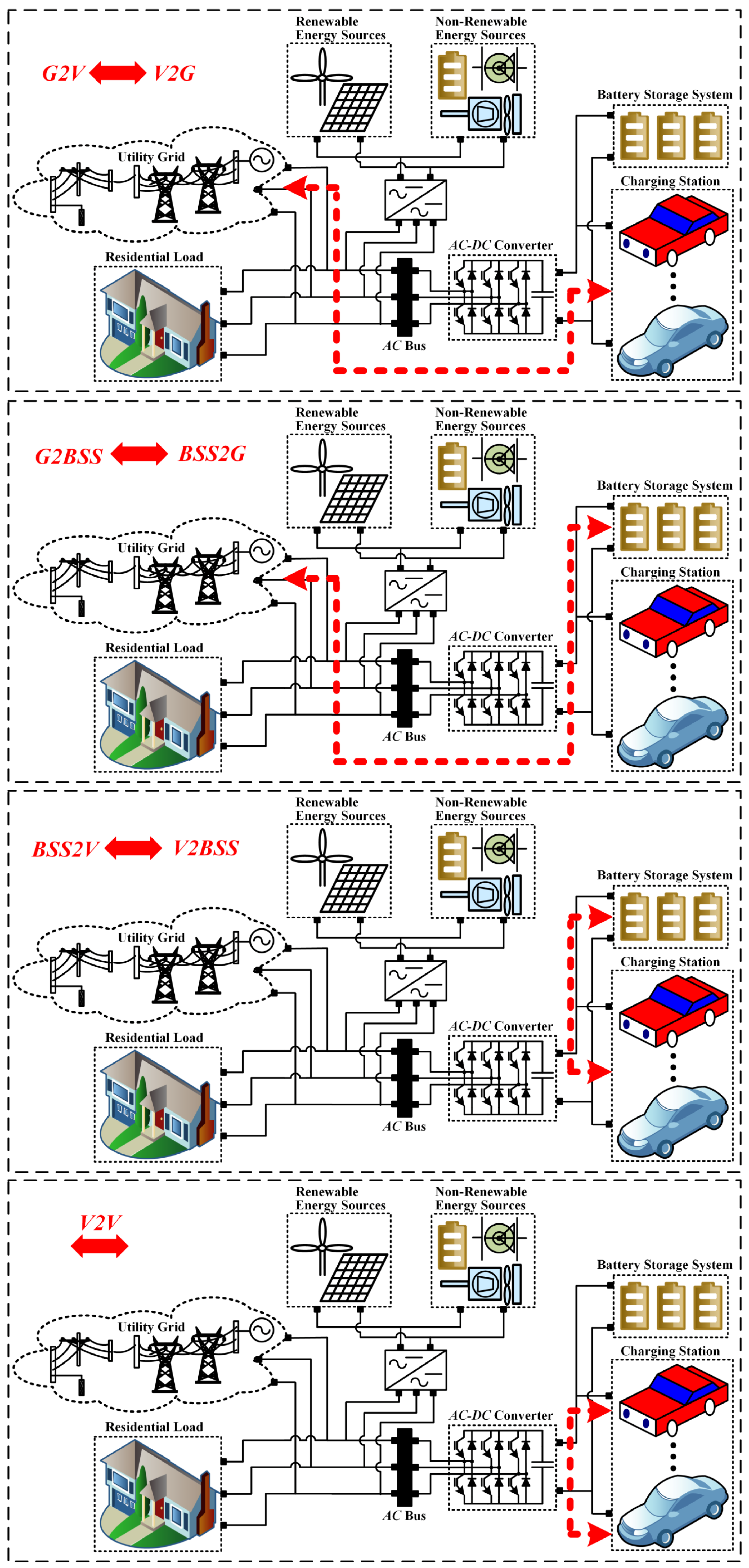
• To design an EMS for optimal power flow between five different PHEVs, CS and grid based on seven different scenarios which include G2V, V2G, grid-to-battery storage system (G2BSS), battery storage system-to-grid (BSS2G), battery storage system-to-vehicle (BSS2V), vehicle-to-battery storage system (V2BSS) and vehicle-to-vehicle (V2V).
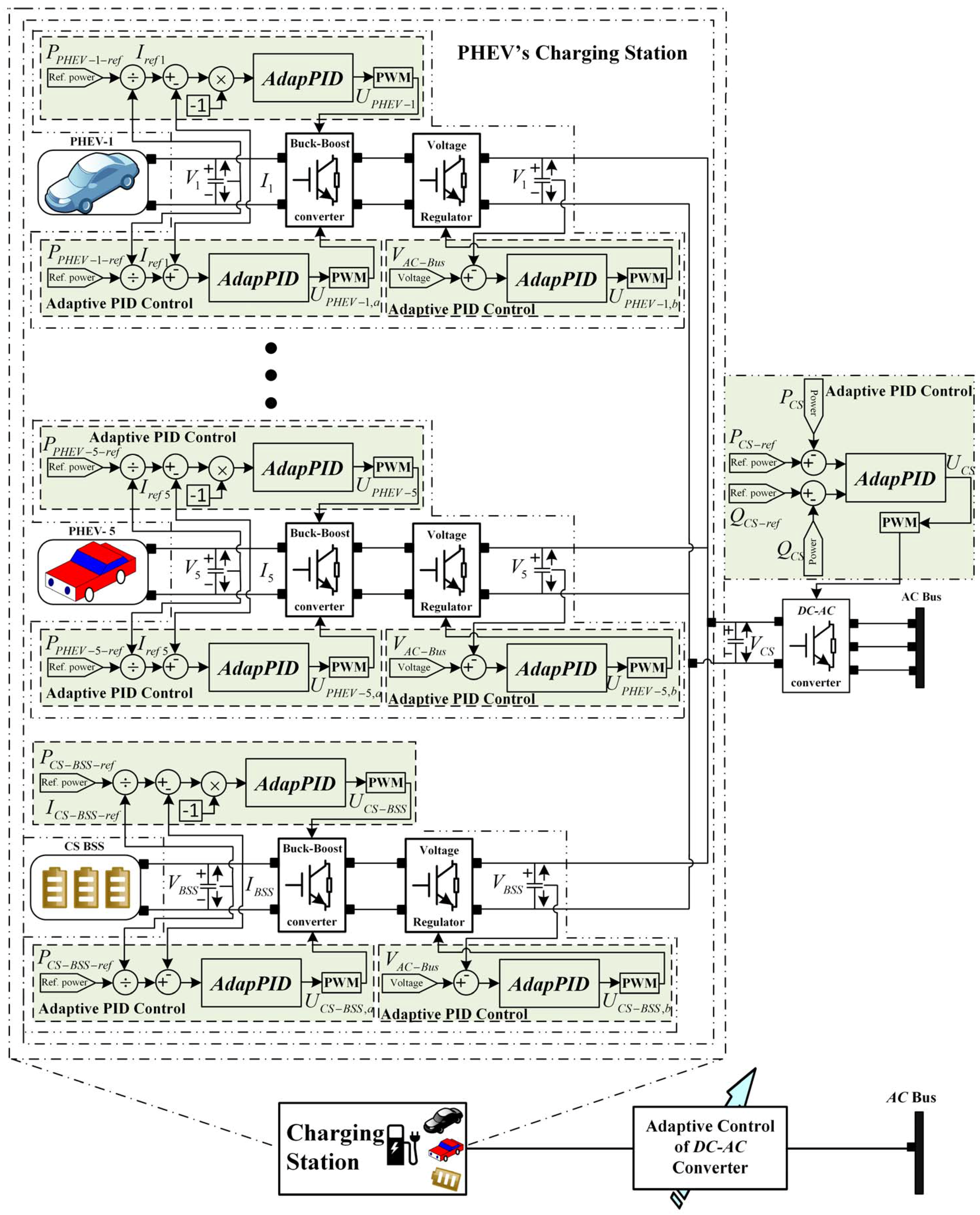
• To design an adaptive control paradigm for a non-renewable energy source (micro-turbine), storage system (battery and super-capacitor), grid side inverter and the charging station (CS converter, battery storage system (BSS), PHEVs).

The rest of the paper is organized into four main sections: Section 2 presents the system description and problem formulation. Section 3 gives the details of the EMS for CS integrated to a grid-connected HPS. Simulation results are discussed in Section 4. Section 5 concludes the outcomes of this research work.

2. System Description and Problem Formulation

The CS shown in Figure 1 is integrated to a grid-connected HPS via an AC bus. Figure 1 represents the proposed charging station (CS) which consists of five different PHEVs and BSS. All the five PHEVs and BSS have a buck-boost converter and a voltage regulator. The buck-boost converter is controlled by two AdapPID controllers. One AdapPID is used in buck mode and other in boost mode. The voltage regulator is also controlled by AdapPID. The CS is connected to AC bus of HPS via DC-AC converter. The DC-AC converter is also controlled by AdapPID. The detail of the stated HPS which consists of renewable, non-renewable energy sources (micro-turbine (MT)), storage system (battery and super-capacitor (SC)), utility grid and CS is given in [4]. In the HPS, there are two types of loads which are connected to AC bus. One is the residential load (P_L) and other is the CS load (P_CS). The power balance equations for the residential and charging station loads are:

$$\Delta P_L(k)=+P_{ES}(k)+P_{Grid}(k)$$

(1)

$$\Delta P_{CS}(k)=+P_{CS-BSS}(k)+{\displaystyle \sum _{i=1}^N{P}_{\stackrel{i}{PHEV}}(k)}+P_{Grid}(k)$$

(2)

where N = 1, 2, …, 5 is the number of PHEVs. The load power, P_L is provided by all renewable, non-renewable energy sources and also by the utility grid. The P_ES(k) is the power delivered by all renewable and non-renewable energy sources. The charging station power, P_CS(k) is provided by charging station BSS (P_C−BSS(k)), PHEVs (P_PHEVs(k)) and from the grid (P_Grid(k)).

2.1. Problem Formulation

The nonlinear HPS with renewable energy sources, non-renewable energy sources, storage system, and CS is mathematically described as:

$$\left[\begin{array}{c}\begin{array}{l}{\widehat{y}}_{RES}(k)\\ y_{NRES}(k)\\ y_{SS}(k)\\ y_{GInv}(k)\end{array}\\ y_{CS}(k)\end{array}\right]=\left[\begin{array}{ccccc}{f}_{NF-RES}(\mathsf{\Omega }(k))& 0& 0& 0& 0\\ 0& f_{NRES}(x(k))& 0& 0& 0\\ 0& 0& f_{SS}(x(k))& 0& 0\\ 0& 0& 0& f_{GInv}(x(k))& 0\\ 0& 0& 0& 0& f_{CS}(x(k))\end{array}\right]$$

(3)

where ${\widehat{y}}_{RES}\left(k\right)=f_{NF-RES}\left(\mathsf{\Omega }\left(k\right)\right)$ represents the auto-regression NeuroFuzzy model of the nonlinear RES which includes variable speed wind-turbine (WT), PV and SOFC. $y_{RES}=f_{NRES}\left(x\left(k\right)\right)$ represents the non-linear model of non-renewable energy sources (NRES) which includes micro-turbines. $y_{SS}=f_{SS}\left(x\left(k\right)\right)$ represents the nonlinear model of the storage system (SS) which includes battery and super-capacitor. $y_{GInv}\left(k\right)=f_{GInv}\left(x\left(k\right)\right)$ represents the non-linear model of the grid side inverter (GInv) and $y_{CS}\left(k\right)=f_{CS}\left(x\left(k\right)\right)$ represents the non-linear model of the PHEVs charging station. Also:

$${\widehat{y}}_{RES}(k)={\left[{\widehat{y}}_{NF-WT}(k){\widehat{y}}_{NF-PV}(k){\widehat{y}}_{NF-SOFC}(k)\right]}^T$$

(4)

where ${\widehat{y}}_{NF-WT}\left(k\right),$ ${\widehat{y}}_{NF-PV}\left(k\right)$ and ${\widehat{y}}_{NF-SOFC}\left(k\right)$ are identified models of WT, PV and SOFC [4]. Similarly:

$$y_{NRES}(k)=[y_{MT}(k)]$$

(5)

$$y_{SS}(k)={[y_{BAT}(k)y_{SC}(k)]}^T$$

(6)

$$y_{GInv}(k)=[y_{GInv}(k)]$$

(7)

$$y_{CS}(k)={[y_{CS-Inv}(k)y_{CS-BSS}(k)y_{\stackrel{i}{PHEVs}}(k)]}^T$$

(8)

where i = 1, 2, …, 5.

$$f_{NF-RES}(\mathsf{\Omega }(k))={[f_{NF-WT}(\mathsf{\Omega }(k))f_{NF-PV}(\mathsf{\Omega }(k))f_{NF-SOFC}(\mathsf{\Omega }(k))]}^T$$

(9)

$$f_{NRES}(x(k))=[f_{MT}(x(k))]$$

(10)

$$f_{SS}(x(k))={[f_{BAT}(x(k))f_{SC}(x(k))]}^T$$

(11)

$$f_{GInv}(x(k))=[f_{GInv}(x(k))]$$

(12)

$$f_{CS}(x(k))={[f_{CS-Inv}(x(k))f_{CS-BSS}(x(k))f_{\stackrel{i}{PHEVs}}(x(k))]}^T$$

(13)

where Ω(k) = [y(k − 1), …, y(k − n), u(k), u(k − 1), …, u(k − m)] and x(k) = [I_MT(k), I_BAT(k), I_SC(k), I_GInv(k), I_CS−Inv(k), I_CS−BSS(k), I_PHEVs(k), V_MT(k), V_BAT(k), V_SC(k), V_GInv(k), V_CS−Inv(k), V_CS−BSS(k), V_PHEVs(k)]^T. The ${\widehat{y}}_{NF-WT}\left(k\right)$ gives predictive output at time step k for a single-input-single-output (SISO) variable speed wind-turbine (VSWT) system. ${\widehat{y}}_{NF-PV}\left(k\right)$ gives the predictive output at time step k for a SISO PV system. ${\widehat{y}}_{NF-SOFC}\left(k\right)$ gives the predictive output at time step k for a SISO SOFC system. The nonlinear dynamic models for the VSWT system, PV system and SOFC system can be captured online if:

$$\underset{t\to \infty }{lim}{\Xi }_{Ide}=\underset{t\to \infty }{lim}\left[\begin{array}{c}{y}_{NF-WT}(k)-{\widehat{y}}_{NF-WT}(k)\\ y_{NF-PV}(k)-{\widehat{y}}_{NF-PV}(k)\\ y_{NF-SOFC}(k)-{\widehat{y}}_{NF-SOFC}(k)\end{array}\right]\Rightarrow {\epsilon }_{Ide}$$

(14)

The control problem is to find an adaptive control law for RES, NRES, SS, GInv and CS given in Equation (3) as follows:

$$\left[\begin{array}{c}\begin{array}{l}{U}_{NF-RES}(k)\\ U_{PID-NRES}(k)\\ U_{PID-SS}(k)\\ U_{PID-GInv}(k)\end{array}\\ U_{PID-CS}(k)\end{array}\right]=\left[\begin{array}{c}{g}_{NF-RES}({\widehat{y}}_{RES}(k),y_{RES-ref}(k))\\ g_{PID-NRES}(y_{NRES}(k),y_{NRES-ref}(k))\\ g_{PID-SS}(y_{SS}(k),y_{SS-ref}(k))\\ g_{PID-GInv}(y_{GInv}(k),y_{GInv-ref}(k))\\ g_{PID-CS}(y_{CS}(k),y_{CS-ref}(k))\end{array}\right]$$

(15)

Equation (15) is used to track the trajectories for the RES, NRES, SS, GInv, CS for all $t\in \left[0,\infty \right]$ as:

$$\underset{t\to \infty }{lim}{\Xi }_{RES}=\underset{t\to \infty }{lim}\left[\begin{array}{c}{y}_{NF-WT}(k)-y_{NF-WT-ref}(k)\\ y_{NF-PV}(k)-y_{NF-PV-ref}(k)\\ y_{NF-SOFC}(k)-y_{NF-SOFC-ref}(k)\end{array}\right]\Rightarrow {\epsilon }_{RES}$$

(16)

$$\underset{t\to \infty }{lim}{\Xi }_{NRES}=\underset{t\to \infty }{lim}\left[y_{NRES}(k)-y_{NRES-ref}(k)\right]\Rightarrow {\epsilon }_{NRES}$$

(17)

$$\underset{t\to \infty }{lim}{\Xi }_{SS}=\underset{t\to \infty }{lim}\left[y_{SS}(k)-y_{SS-ref}(k)\right]\Rightarrow {\epsilon }_{SS}$$

(18)

$$\underset{t\to \infty }{lim}{\Xi }_{GInv}=\underset{t\to \infty }{lim}\left[y_{GInv}(k)-y_{GInv-ref}(k)\right]\Rightarrow {\epsilon }_{GInv}$$

(19)

$$\underset{t\to \infty }{lim}{\Xi }_{CS}=\underset{t\to \infty }{lim}\left[y_{CS}(k)-y_{CS-ref}(k)\right]\Rightarrow {\epsilon }_{CS}$$

(20)

where ${\epsilon }_{RES}$, ${\epsilon }_{NRES}$, ${\epsilon }_{SS}$, ${\epsilon }_{GInv}$, ${\epsilon }_{CS}$ are the small tracking errors:

$$y_{NRES}(k)=[y_{MT}(k)]=\left[P_{MT}(k)\right]$$

(21)

$$y_{NRES-ref}(k)=\left[y_{MT-ref}(k)\right]=\left[P_{MT-ref}(k)\right]$$

(22)

$$y_{SS}(k)={\left[y_{BAT}(k),y_{SC}(k)\right]}^T={\left[P_{BAT}(k),P_{SC}(k)\right]}^T$$

(23)

$$y_{SS-ref}(k)={\left[y_{BAT-ref}(k),y_{SC-ref}(k)\right]}^T={\left[P_{BAT-ref}(k),P_{SC-ref}(k)\right]}^T$$

(24)

$$y_{GInv}(k)=\left[P_{GInv}(k)\right]$$

(25)

$$y_{GInv-ref}(k)=\left[P_{GInv-ref}(k)\right]$$

(26)

$$y_{CS}(k)={\left[y_{CS-Inv}(k),y_{CS-BSS}(k),y_{\stackrel{i}{PHEVs}}(k)\right]}^T={\left[P_{CS-Inv}(k),P_{CS-BSS}(k),P_{\stackrel{i}{PHEVs}}(k)\right]}^T$$

(27)

$$\begin{array}{ll}\hfill y_{CS-ref}(k)& ={\left[y_{CS-Inv-ref}(k),y_{CS-BSS-ref}(k),y_{\stackrel{i}{PHEVs-ref}}(k)\right]}^T\hfill \\ & ={\left[P_{CS-Inv-ref}(k),P_{CS-BSS-ref}(k),P_{\stackrel{i}{PHEVs-ref}}(k)\right]}^T\hfill \end{array}$$

(28)

Similarly:

$$U_{NF-RES}(k)={[U_{NF-WT}(k)U_{NF-PV}(k)U_{NF-SOFC}(k)]}^T$$

(29)

$$U_{PID-NRES}(k)=[U_{PID-NRES}(k)]$$

(30)

$$U_{PID-SS}(k)={[U_{PID-BAT}(k)U_{PID-SC}(k)]}^T$$

(31)

$$U_{PID-GInv}(k)=[U_{PID-GInv}(k)]$$

(32)

$$U_{PID-CS}(k)={[U_{PID-CS-Inv}(k)U_{PID-CS-BSS}(k)U_{\stackrel{i}{PID-PHEVs}}(k)]}^T$$

(33)

The equation for $U_{NF-RES}\left(k\right)$ has been solved in [4].

2.2. Adaptive PID Control System Design

The adaptive control law $U_{SAdapPID}\left(k\right)\in \left[U_{PID-NRES}\left(k\right),U_{PID-SS}\left(k\right),U_{PID-GInv}\left(k\right),U_{PID-CS}\left(k\right)\right]$ to track the trajectories $y_{NRES-ref}\left(k\right)$, $y_{SS-ref}\left(k\right)$, $y_{GInv-ref}\left(k\right)$, $y_{CS-ref}\left(k\right)$ is given as:

$$U_{AdapPID}(k)=K_{P-Adap}(k)e(k)+K_{I-Adap}(k){\displaystyle \int \left(e(k)\right)dt}+K_{D-Adap}(k)\frac{d\left(e(k)\right)}{dt}$$

(34)

where $K_{P-Adap}\in [K_{P-Adap-NRES},K_{P-Adap-SS},K_{P-Adap-GInv},K_{P-Adap-CS}],$ $K_{I-Adap}\in [K_{I-Adap-NRES},K_{I-Adap-SS},K_{I-Adap-GInv},K_{I-Adap-CS}]$ and $K_{D-Adap}\in [K_{D-Adap-NRES},K_{D-Adap-SS},K_{D-Adap-GInv},K_{D-Adap-CS}]$ are proportional, integral and derivative constants. The cost function for achieving the adaptive control law to solve the tracking problem for NRES, SS, GInv and CS is given as:

$$\min \downarrow J(k)=\frac{1}{2}\left[J_{NRES}^2(k),J_{SS}^2(k),J_{GInv}^2(k),J_{CS}^2(k)\right]$$

(35)

Subject to:

$$\{\begin{array}{l}NRES\Rightarrow \{\begin{array}{l}{K}_{P-Adap-MT,\min }\le K_{P-Adap-MT}\le K_{P-Adap-MT,\max }\\ K_{I-Adap-MT,\min }\le K_{I-Adap-MT}\le K_{I-Adap-MT,\max }\\ K_{D-Adap-MT,\min }\le K_{D-Adap-MT}\le K_{D-Adap-MT,\max }\end{array}\\ SS\Rightarrow \{\begin{array}{l}{K}_{P-Adap-BAT,\min }\le K_{P-Adap-BAT}\le K_{P-Adap-BAT,\max }\\ K_{I-Adap-BAT,\min }\le K_{I-Adap-BAT}\le K_{I-Adap-BAT,\max }\\ K_{D-Adap-BAT,\min }\le K_{D-Adap-BAT}\le K_{D-Adap-BAT,\max }\\ K_{P-Adap-SC,\min }\le K_{P-Adap-SC}\le K_{P-Adap-SC,\max }\\ K_{I-Adap-SC,\min }\le K_{I-Adap-SC}\le K_{I-Adap-SC,\max }\\ K_{D-Adap-SC,\min }\le K_{D-Adap-SC}\le K_{D-Adap-SC,\max }\end{array}\\ GInv\Rightarrow \{\begin{array}{l}{K}_{P-Adap-GInv,\min }\le K_{P-Adap-GInv}\le K_{P-Adap-GInv,\max }\\ K_{I-Adap-GInv,\min }\le K_{I-Adap-GInv}\le K_{I-Adap-GInv,\max }\\ K_{D-Adap-GInv,\min }\le K_{D-Adap-GInv}\le K_{D-Adap-GInv,\max }\end{array}\\ CS\Rightarrow \{\begin{array}{l}{K}_{P-Adap-CS-Inv,\min }\le K_{P-Adap-CS-Inv}\le K_{P-Adap-CS-Inv,\max }\\ K_{I-Adap-CS-Inv,\min }\le K_{I-Adap-CS-Inv}\le K_{I-Adap-CS-Inv,\max }\\ K_{D-Adap-CS-Inv,\min }\le K_{D-Adap-CS-Inv}\le K_{D-AdapCS-Inv,\max }\\ K_{P-Adap-CS-BSS,\min }\le K_{P-Adap-CS-BSS}\le K_{P-Adap-CS-BSS,\max }\\ K_{I-Adap-CS-BSS,\min }\le K_{I-Adap-CS-BSS}\le K_{I-Adap-CS-BSS,\max }\\ K_{D-Adap-CS-BSS,\min }\le K_{D-Adap-CS-BSS}\le K_{D-Adap-CS-BSS,\max }\\ K_{P-Adap-\stackrel{i}{PHEVs},\min }\le K_{P-Adap-\stackrel{i}{PHEVs}}\le K_{P-Adap-\stackrel{i}{PHEVs},\max }\\ K_{I-Adap-\stackrel{i}{PHEVs},\min }\le K_{I-Adap-\stackrel{i}{PHEVs}}\le K_{I-Adap-\stackrel{i}{PHEVs},\max }\\ K_{D-Adap-\stackrel{i}{PHEVs},\min }\le K_{D-Adap-\stackrel{i}{PHEVs}}\le K_{D-Adap-\stackrel{i}{PHEVs},\max }\end{array}\end{array}$$

where:

$$J_{NRES}(k)=P_{NRES}(k)-P_{NRES-ref}(k)$$

(36)

$$J_{SS}(k)=\{\begin{array}{l}{y}_{BAT}(k)-y_{BAT-ref}(k)\\ y_{SC}(k)-y_{SC-ref}(k)\end{array}$$

(37)

$$J_{GInv}(k)=y_{GInv}(k)-y_{GInv-ref}(k)$$

(38)

$$J_{CS}(k)=\{\begin{array}{l}{y}_{CS-Inv}(k)-y_{CS-Inv-ref}(k)\\ y_{CS-BSS}(k)-y_{CS-BSS-ref}(k)\\ y_{\stackrel{i}{PHEVs}}(k)-y_{\stackrel{i}{PHEVs}-ref}(k)\end{array}$$

(39)

The generalized update law for the parameter $K_{Adap}\in \left\{K_{P-Adap},K_{I-Adap},K_{D-Adap}\right\}$ is given as:

$$K_{Adap}(k+1)=K_{Adap}(k)+{\alpha }_{Adap}\frac{\partial J(k)}{\partial K_{Adap}(k)}$$

(40)

where ${\alpha }_{Adap}$ is the learning rate, i.e., $0<{\alpha }_{Adap}<1$. The gradient descent algorithm is used to update the $K_{Adap}$ as follows:

$$\frac{\partial J(k)}{\partial K_{Adap}(k)}=-\frac{\partial J(k)}{\partial y(k)}\frac{\partial y(k)}{\partial U_{AdapPID}(k)}\frac{\partial U_{AdapPID}(k)}{\partial K_{Adap}(k)}$$

(41)

where $y(k)=\left[y_{NRES}(k),y_{SS}(k),y_{GInv}(k),y_{CS}(k)\right]$, $\frac{\partial J(k)}{\partial y(k)}=-e(k)$ and $\frac{\partial y(k)}{\partial U_{AdapPID}(k)}=1$ [32]. The term $\frac{\partial U_{AdapPID}(k)}{\partial K_{Adap}(k)}$ which is associated with $K_{P-Adap},K_{I-Adap},K_{D-Adap}$ can be calculated as $\frac{\partial U_{AdapPID}(k)}{\partial K_{P-Adap}(k)}=e(k)$, $\frac{\partial U_{AdapPID}(k)}{\partial K_{I-Adap}(k)}={\displaystyle \int e(k)dt}$ and $\frac{\partial U_{AdapPID}(k)}{\partial K_{D-Adap}(k)}=\frac{d(e(k))}{dt}$. The error e(k) is calculated as:

$$e(k)=y(k)-y_{ref}(k)$$

(42)

where $y_{ref}(k)=\left[y_{NRES-ref}(k),y_{SS-ref}(k),y_{GInv-ref}(k),y_{CS-ref}(k)\right].$ Therefore, the update equations for $K_{P-Adap},K_{I-Adap},K_{D-Adap}$ are:

$$K_{P-Adap}(k+1)=K_{P-Adap}(k)+{\alpha }_{Adap}{e}^2(k)$$

(43)

$$K_{I-Adap}(k+1)=K_{I-Adap}(k)+{\alpha }_{Adap}e(k){\displaystyle \int e(k)dt}$$

(44)

$$K_{D-Adap}(k+1)=K_{D-Adap}(k)+{\alpha }_{Adap}e(k)\frac{d(e(k))}{dt}$$

(45)

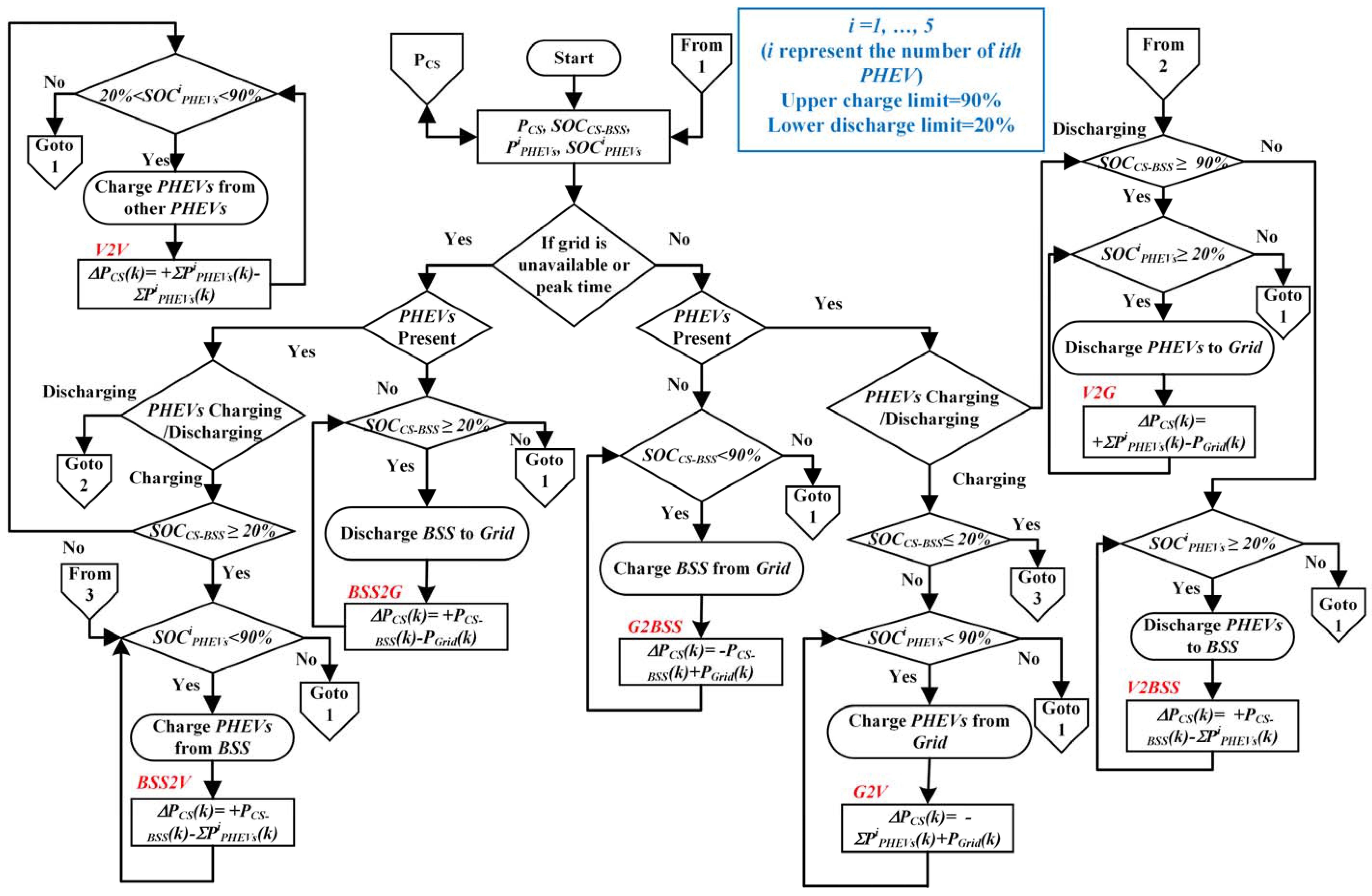
3. Energy Management System for the Charging Station

The EMS ensures the continuous and reliable power supply to the CS load, i.e., $P_{CS}(k)$. To satisfy the $P_{CS}(k)$ and enhance the HPS reliability, the EMS offers seven different modes of operation which include G2V, V2G, G2BSS, BSS2G, BSS2V, V2BSS and V2V. The detail of these modes are as follows:

• Mode-1: G2V: $V_{Grid}(k)>V_{CS}(k)\&SO{C}_{CS-BSS}(k)\le 20\%\&SO{C}_{\stackrel{i}{PHEVs}}(k)<90\%$

Where $V_{Grid}(k)$ is the grid voltage, $V_{CS}(k)$ is the CS voltage, $SO{C}_{CS-BSS}(k)$ is the SOC of BSS and $SO{C}_{\stackrel{i}{PHEVs}}(k)$ is the SOC of the ith PHEV. In this mode, the PHEVs are charged with the power taken from the utility grid. The SOC of BSS is less than 20%. The PHEVs are preferred to charge during off peak hours of the grid. The power balance equation for G2V mode is given as:

$$\Delta P_{CS}(k)=-{\displaystyle \sum _{i=1}^N{P}_{\stackrel{i}{PHEVs}}(k)}+P_{Grid}(k)$$

(46)

A ‘+’ symbol represents the power delivered by the source and a ‘−’ symbol represents the power absorbed by the load.

• Mode-2: V2G: $V_{CS}(k)>V_{Grid}(k)\&SO{C}_{CS-BSS}(k)\ge 90\%\&SO{C}_{\stackrel{i}{PHEVs}}(k)\ge 20\%$

During the peak demand hours of the grid, the PHEVs help to reduce the stress on the grid. The PHEVs are discharged and deliver the power to the utility grid via AC bus. The power balance equation for this mode of operation is given as:

$$\Delta P_{CS}(k)=+{\displaystyle \sum _{i=1}^N{P}_{\stackrel{i}{PHEVs}}(k)}-P_{Grid}(k)$$

(47)

• Mode-3: G2BSS: $V_{Grid}(k)>V_{CS}(k)\&SO{C}_{CS-BSS}(k)<90\%\&SO{C}_{\stackrel{i}{PHEVs}}(k)\ge 20\%$

During this mode of operation, the grid is having off peak hours. Therefore, the utility grid delivers the power to charge the BSS. The power balance equation is given as follows:

$$\Delta P_{CS}(k)=-P_{CS-BSS}(k)+P_{Grid}(k)$$

(48)

• Mode-4: BSS2G: $V_{CS}(k)>V_{Grid}(k)\&SO{C}_{CS-BSS}(k)\ge 20\%\&SO{C}_{\stackrel{i}{PHEVs}}(k)\ge 20\%$

The operation of this mode is similar to V2G mode but the BSS is in discharge mode in-spite of PHEVs. The BSS also supplies the power to the utility grid during its peak demand hours. This mode has the following power balance equation.

$$\Delta P_{CS}(k)=+P_{CS-BSS}(k)-P_{Grid}(k)$$

(49)

• Mode-5: BSS2V: $V_{CS}(k)=V_{Grid}(k)\&SO{C}_{CS-BSS}(k)\ge 20\%\&SO{C}_{\stackrel{i}{PHEVs}}(k)<90\%$

In this mode of operation, the utility grid is at peak demand hours. The SOC of BSS is greater than 20%. Therefore, the PHEVs are charged from the BSS. The power balance equation for this mode of operation is defined as:

$$\Delta P_{CS}(k)=+P_{CS-BSS}(k)-{\displaystyle \sum _{i=1}^N{P}_{\stackrel{i}{PHEVs}}(k)}$$

(50)

• Mode-6: V2BSS: $V_{CS}(k)=V_{Grid}(k)\&SO{C}_{CS-BSS}(k)<90\%\&SO{C}_{\stackrel{i}{PHEVs}}(k)\ge 20\%$

In this mode, the PHEVs are discharged and they deliver the power to charge the BSS. The power balance equation is given as:

$$\Delta P_{CS}(k)=-P_{CS-BSS}(k)+{\displaystyle \sum _{i=1}^N{P}_{\stackrel{i}{PHEVs}}(k)}$$

(51)

• Mode-7: V2V: $V_{CS}(k)=V_{Grid}(k)\&SO{C}_{CS-BSS}(k)\le 20\%\&20\%\le SO{C}_{\stackrel{i}{PHEVs}}(k)\le 90\%$

During this mode of operation, the PHEV demand is fulfilled by another PHEV. The charging power of the PHEV is equal or greater than the discharging power of the PHEV. The power balance equation for V2V mode is given as follow:

$$\Delta P_{CS}(k)=+{\displaystyle \sum _{i=1}^N{P}_{\stackrel{i}{PHEVs}}(k)}-{\displaystyle \sum _{i=1}^N{P}_{\stackrel{i}{PHEVs}}(k)}$$

(52)

The flow chart for the charging station EMS is shown in Figure 2.

All the seven modes of EMS in the HPS are depicted in Figure 3.

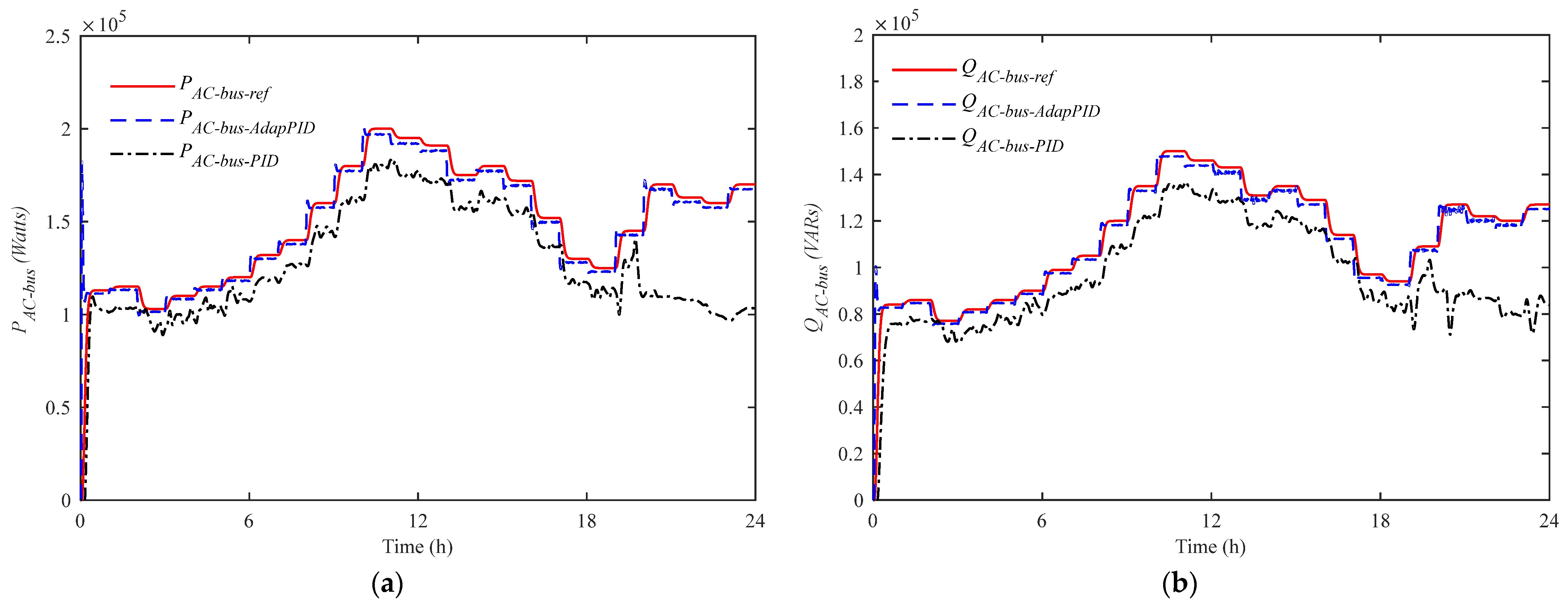
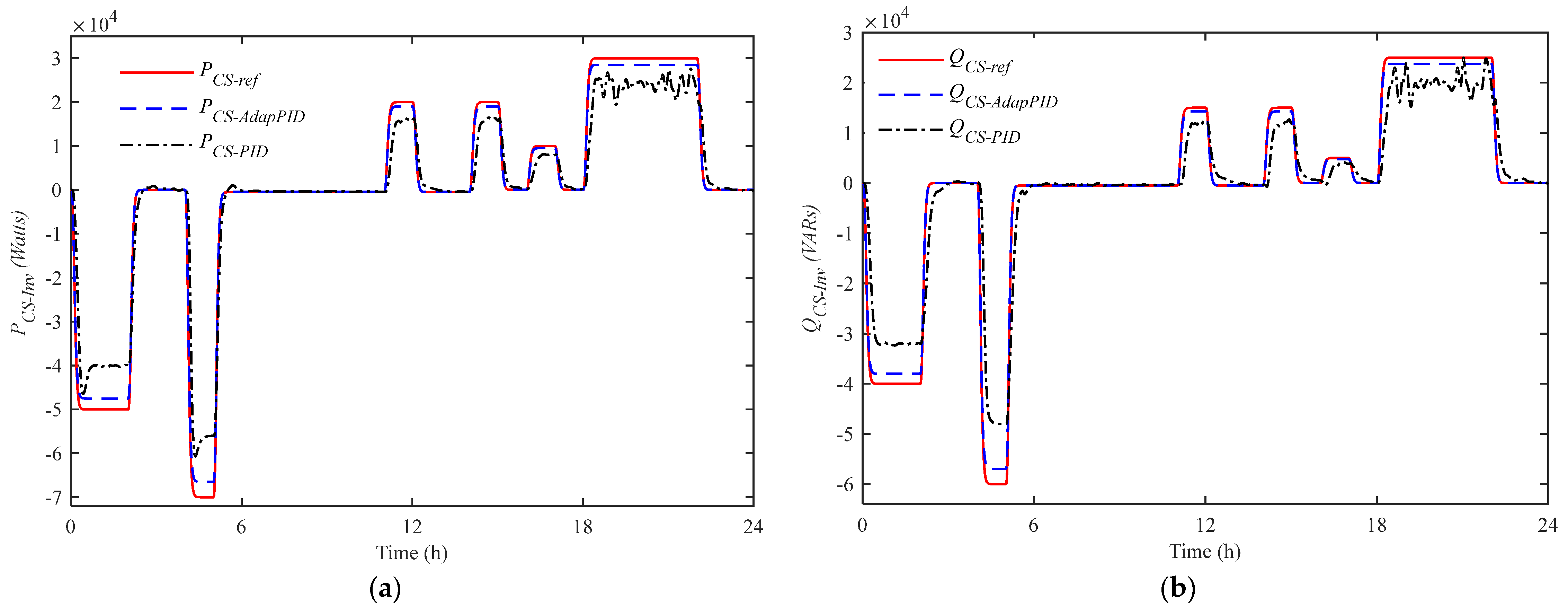
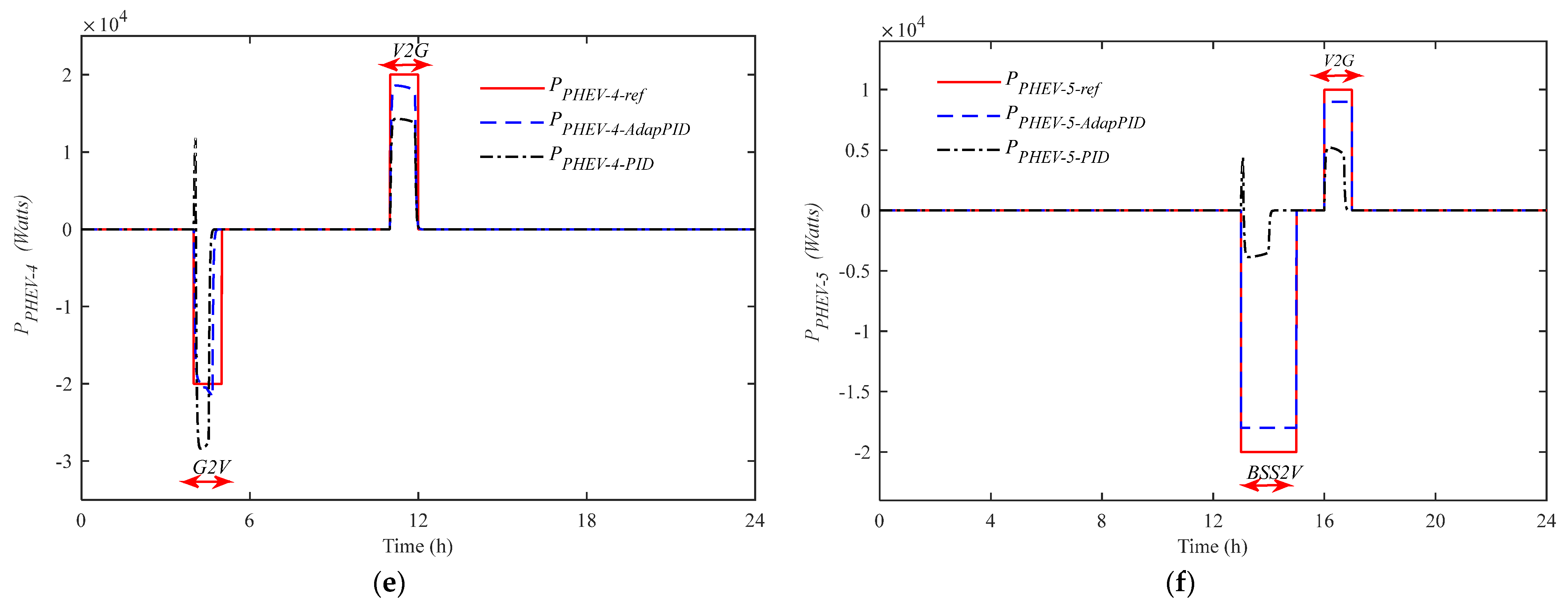
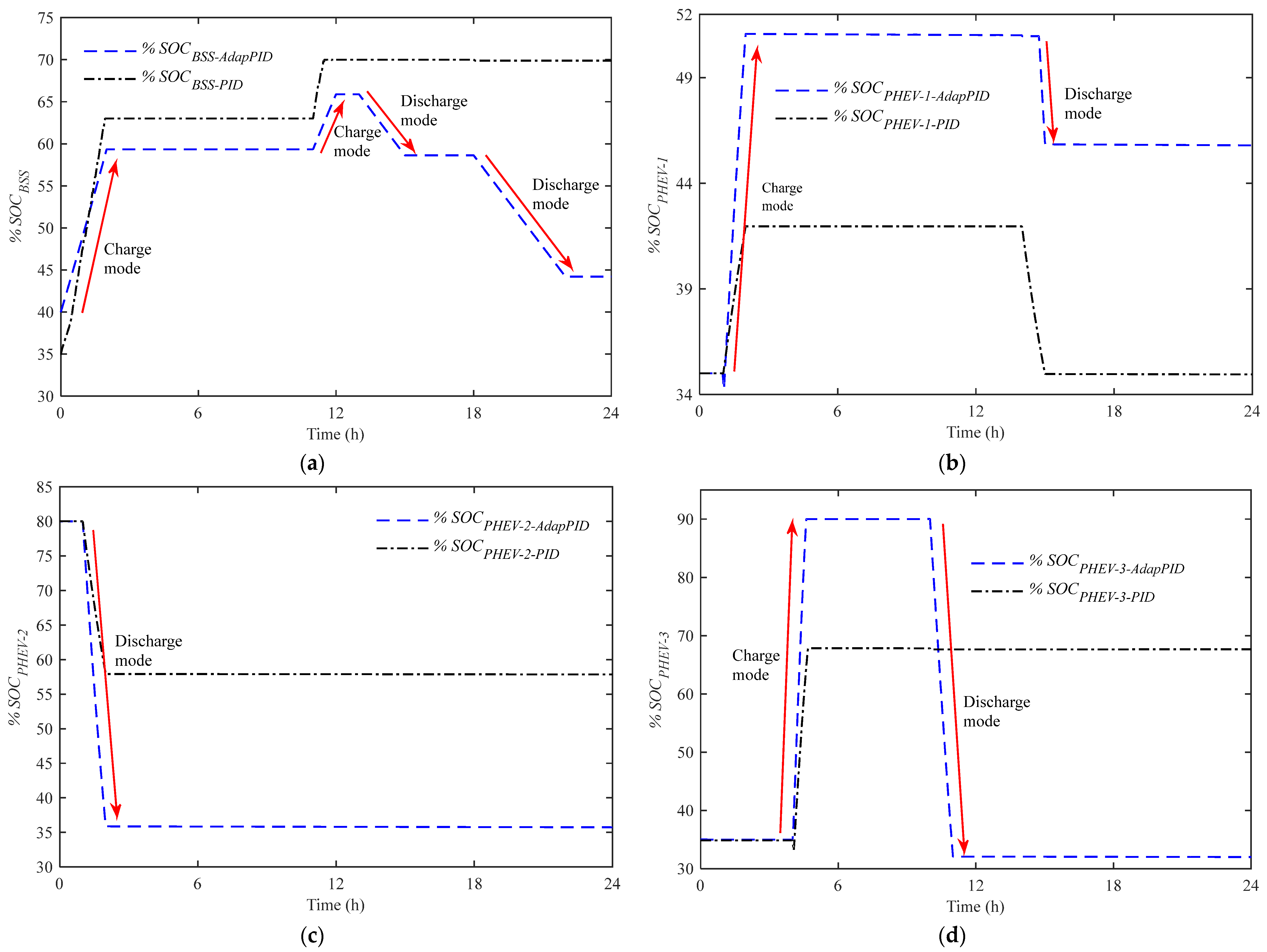
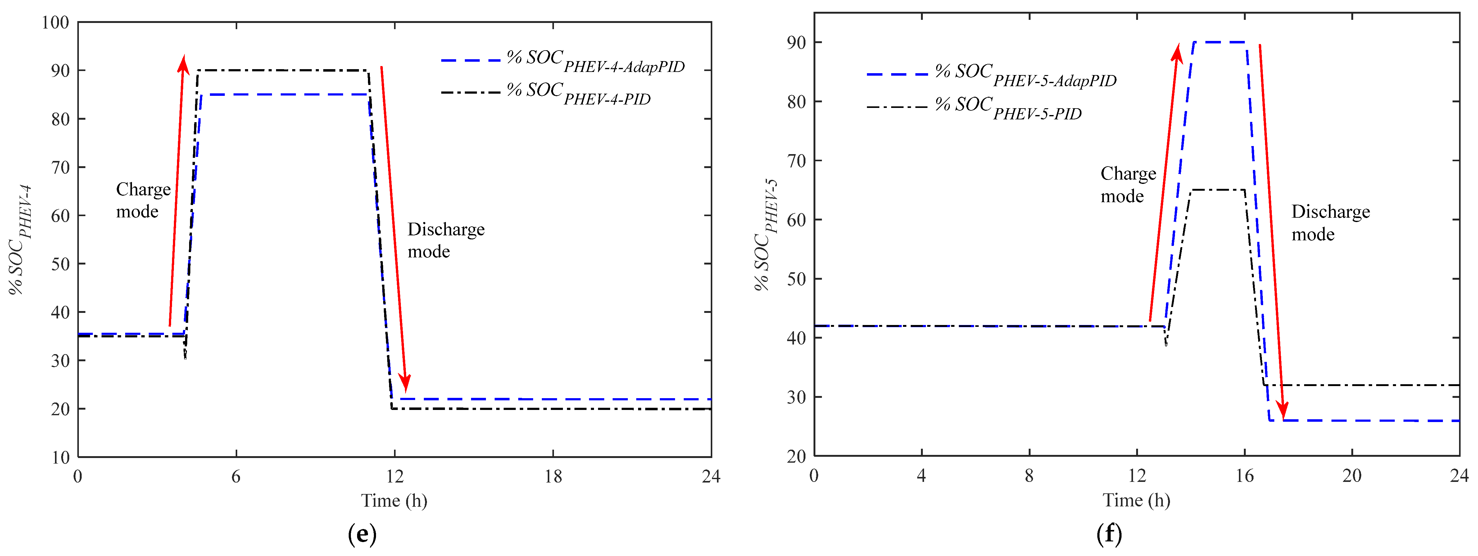
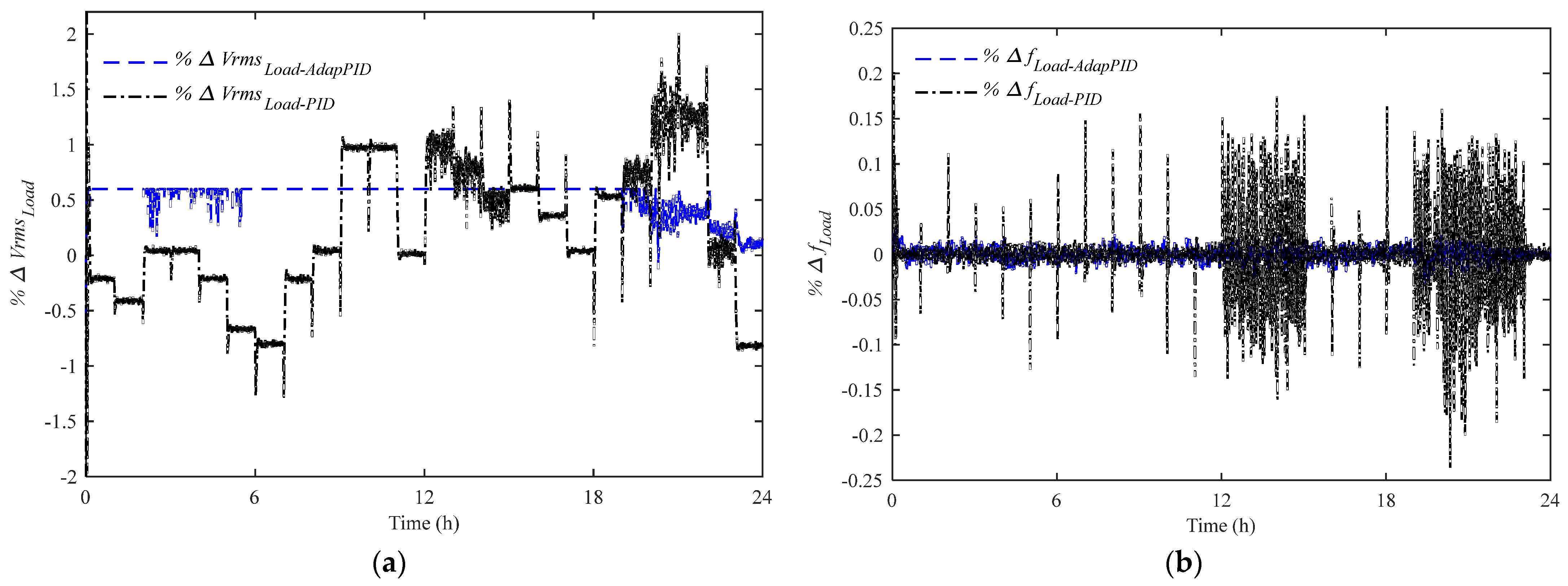
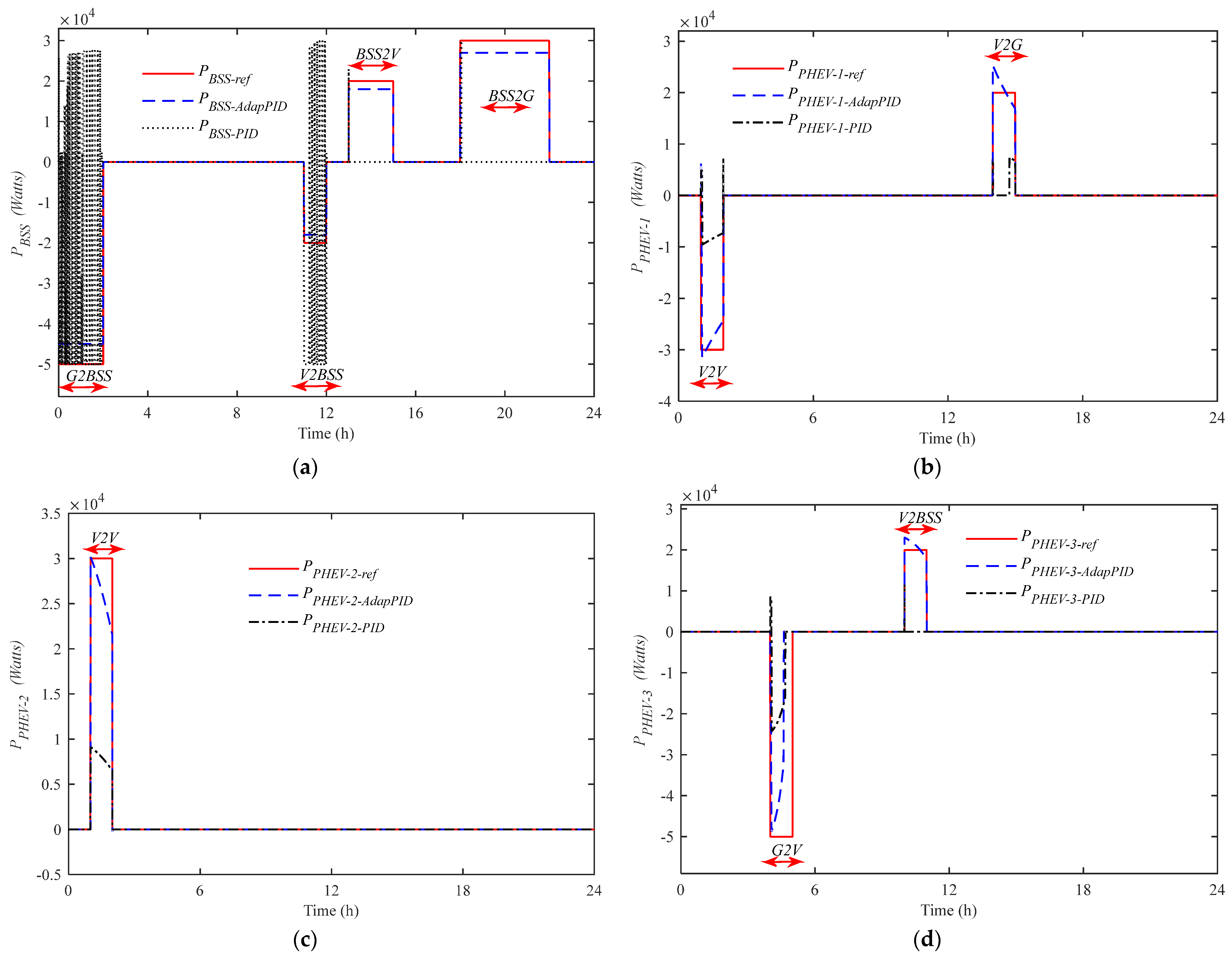
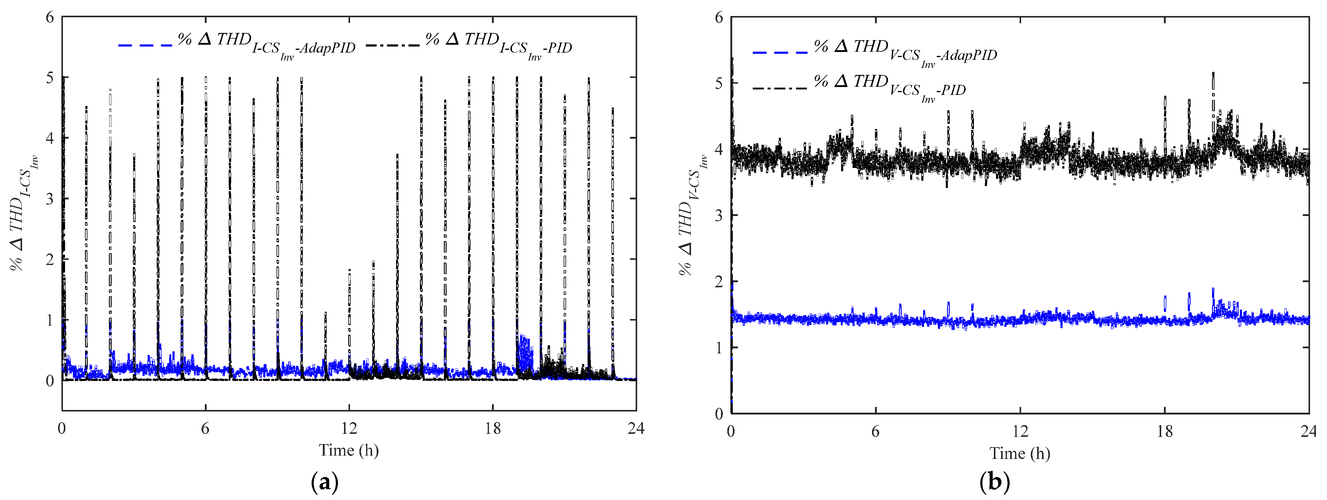
4. Results and Discussion

The performance of the CS in a grid-connected HPS has been evaluated with both adaptive and conventional approaches in MATLAB/Simulink R2015a (The MathWork Inc, Natick, MA, USA). The HPS consists of 11 kV of the grid, 100 kW of wind generation, 260 kW of PV, 200 kW of SOFC, 150 kW of the electrolyzer and 200 kVA of MT. The backup sources include battery (200 Ah) and SC (165 F). All the energy sources are modeled for the accumulative dynamic residential and charging station load. Defense Housing Authority (DHA), Islamabad, Pakistan, is taken as a case study. The hourly basis wind speed (m/s), irradiance (W/m²) and ambient temperature (°C) levels are recorded by the Pakistan Meteorological Department (PMD). There are two types of loads in the HPS which are residential load and CS load. The residential load and CS load are connected to AC bus. The power to the total load (P_L + P_CS) is provided by all the RES, NRES, SS, CS and the utility grid via AC bus. The active and reactive powers of AC bus is shown in Figure 4a,b. The AdapPID controller adequately controls the grid inverter to track the active and reactive power reference trajectories to ensure energy balance between generation and load. The steady-state error (SSE) with AdapPID control is 1 kW, whereas, PID control has 6.68 kW. The undershoot with AdapPID control is 2% while the PID control has 66%.

The DC-AC converter of the CS is responsible for bidirectional power flow between CS and the utility grid. In G2BSS, BSS2G, G2V and V2G modes of operation, the DC-AC converter of CS is involved. The active and reactive powers of the DC-AC converter for CS is shown in Figure 5. During 0–2 h, the CS takes 50 kW power from the utility grid. This 50 kW power is used to charge the BSS. In time interval 4–5 h, the CS utilizes 70 kW power from the grid in G2V mode. During time intervals 11–12, 14–15 and 16–17, the CS delivers the power to the utility grid in V2G mode. In time interval 18–22 h, the CS delivers 30 kW power to the utility grid in BSS2G mode. The AdapPID closely tracks the active and reactive powers of CS.

The AdapPID control scheme adequately manipulates the charging station DC-AC inverter to track the CS active and reactive power reference trajectories. It results in less oscillations and SSE error as compared to conventional PID controller as shown in Figure 5.

The CS consists of five different PHEVs and a BSS. These PHEVs and BSS act as either loads or energy sources. Each PHEV/BSS has its own buck-boost converter. The buck mode is used to charge the PHEV/BSS, whereas, the boost mode is used to discharge the PHEV/BSS. The buck-boost converter is controlled by AdapPID. Based on the reference power, each buck-boost converter extracts or delivers the power to the PHEVs/BSS. To meet the dynamic CS load, the EMS offers seven different modes of operation which include G2V, V2G, G2BSS, BSS2G, BSS2V, V2BSS and V2V as shown in Figure 6.

Figure 6a represents the BSS power. During off peak hours of the grid, i.e., 0–2 h, the G2BSS mode is activated. The BSS is charged from the grid power. The BSS utilizes 50 kW power from the grid. During 11–12 h, the BSS is again in charge mode and the V2BSS mode is activated. The PHEV-3 delivers 20 kW power to charge the BSS as shown in Figure 6d. For t = 13–15 h, the BSS2V mode is activated. During this mode of operation, the BSS delivers 20 kW power to PHEV-5 as shown in Figure 6f. During 18–22 h, the BSS2G mode is ON, becasuse the grid is having peak demand hours and the BSS tries to reduce the stress on the grid. The BSS delivers 30 kW power to the utility grid. Figure 6b shows the power of PHEV-1. PHEV-1 is charged from PHEV-2 during 1–2 h in V2V mode. PHEV-2 delivers 30 kW power to the PHEV-1 as shown in Figure 6b,c. The PHEV-1 is in V2G mode during 14–15 h as shown in Figure 6b. During this mode of operation, the PHEV-1 delivers 20 kW power to the utility grid via DC-AC converter of the CS. Figure 6d shows the PHEV-3 power. During 4–5 h, the PHEV-3 is charged from the grid in G2V mode. The grid is having off peak hours, therefore, the PHEV-3 utilizes 50 kW power from the grid. During 10–11 h, the PHEV-3 delivers the power to the BSS in V2BSS mode.Figure 6e shows the PHEV-4 power. The PHEV-4 utilizes 20 kW power from the grid during 4–5 h. In this time interval, the G2V mode is activated. For the peak demand hours of the grid, i.e., 11–12 h, the V2G mode is ON. The PHEV-4 delivers 20 kW power to the utility grid. Figure 6f shows the power of PHEV-5. During 13–15 h, the BSS2V mode is ON and the PHEV-5 is charged from the BSS power. For t = 16–17 h, the V2G mode is activated. In this time interval, the PHEV-5 delivers 10 kW power to the utility grid. The BSS and PHEVs powers are more accurately tracked with AdapPID as compared to PID, because the AdapPID has smaller overshoot, undershoot and SSE as shown in Figure 6. While the conventional PID most of the time loses tracking as shown in Figure 6a,d. Similarly, the undershoot is high with PID as shown in Figure 6b–e.

The corresponding SOCs during charge/discharge mode of the BSS and PHEVs are shown in Figure 7. All the PHEVs and BSS are allowed to discharge and charge within 20% < SOC < 90%. In Figure 7a, for t = 0–2 h, the BSS is in charge mode and the SOC of the BSS increases from 40% to 59% with AdapPID. During the time interval 11–12 h, the BSS is again in charge mode and the SOC increases from 59% to 65.88%. In the next time interval, i.e., 13–15 h when the BSS is in discharge mode the SOC of BSS decreases from 65.88% to 58.63%. During 18–22 h, the BSS is again in discharge mode and the SOC decreases from 58.63% to 44.21%. Figure 7b represents the SOC for charge/discharge mode of the PHEV-1. During 1–2 h, the PHEV-1 is in charge mode and the SOC increases from 35% to 51%. BSS

In the time interval 14–15 h, the PHEV-1 is discharged and the SOC decreases from 51% to 45.84%. The PHEV-2 is in discharge mode during 1–2 h and the SOC of the vehicle decreases from 80% to 35.87% as shown in Figure 7c. The SOC of PHEV-3 is shown in Figure 7d. During 4–5 h, the PHEV-3 is in charge mode. In this time interval, the SOC of PHEV-3 increases from 35% to 90%. Similarly, in interval 10–11 h, the PHEV-3 is in discharge mode and the SOC decreases from 90% to 32%. Figure 7e represents the SOC of PHEV-4. During 4–5 h, the PHEV-4 is in charge mode and the SOC of PHEV-4 increases from 35% to 85%. Similarly, in interval 11–12 h, the PHEV-4 is in discharge mode and the SOC decreases from 85% to 21%. Figure 7f represents the SOC of PHEV-5. During 13–15 h, the PHEV-5 is in charge mode and the SOC of PHEV-5 increases from 42% to 90%.

Similarly, in interval 16–17 h, the PHEV-5 is in discharge mode and the SOC decreases from 90% to 26%. The SOCs of PHEVs are also accurately acquired with AdapPID as shown in Figure 7. While the conventional PID most of the time loses tracking as shown in Figure 7a,d.

The reference power transfer levels for BSS and PHEVs are shown in

Table 1. Reference power transfer levels in kW for respective vehicles and hours.

Vehicle	t1	t2	t3	t4	t5	t6	t7	t8	t9	t10	t11	t12	t13	t14	t15	t16	t17	t18	t19	t20	t21	t22	t23	t24
BSS	−50	−50	0	0	0	0	0	0	0	0	−20	0	+20	+20	0	0	0	+30	+30	+30	+30	0	0	0
PHEV-1	0	−30	0	0	0	0	0	0	0	0	0	0	0	+20	0	0	0	0	0	0	0	0	0	0
PHEV-2	0	+30	0	0	0	0	0	0	0	0	0	0	0	0	0	0	0	0	0	0	0	0	0	0
PHEV-3	0	0	0	−50	0	0	0	0	0	+20	0	0	0	0	0	0	0	0	0	0	0	0	0	0
PHEV-4	0	0	0	−20	0	0	0	0	0	0	+20	0	0	0	0	0	0	0	0	0	0	0	0	0
PHEV-5	0	0	0	0	0	0	0	0	0	0	0	0	−20	−20	0	+10	0	0	0	0	0	0	0	0

. The reference power transfer levels for BSS and PHEVs are assumed in this study. These power transaction levels are assumed to maximize the revenue. This profit is possible when all the PHEVs and BSS have access to the real-time electricity price information which varies throughout the 24 h. However, the process of deriving such schedule is not within the scope of this study.

To evaluate the HPS stability and power quality, different parameters are also calculated which include total harmonic distortions (THD) for CS converter current and voltage, load rms voltage, and load frequency. The HPS stability and power quality assumption are applied according to IEEE Std. 1547 [33]. The percentage change in THDs for both current and voltage is shown in Figure 8. The percentage change in load rms voltage and frequency is shown in Figure 9. The AdapPID controller has a flat profile as compared to PID controller for the percentage change in current THD, voltage THD, load rms voltage and frequency. The charging station with AdapPID control injects less harmonics into the AC bus which greatly enhances the quality of load voltage and current. It also keeps the system frequency well within the IEEE Std. 1547 [33].

5. Conclusions

In this article, an energy management system and control of PHEVs of a charging station in a hybrid power system has been presented. The charging station consists of DC-DC converters for PHEVs and AC-DC converter for interfacing to AC bus. The renewable energy sources are adaptively controlled to extract maximum power. In the simulation, G2V, V2G, G2BSS, BSS2G, BSS2V, V2BSS and V2V operations of the charging station have been simulated. Best performance has been demonstrated in all modes of operation of charging station by adaptively controlled DC-DC and AC-DC converters. It is obvious from the results that the adaptive PID control system adequately tracks the demanded/delivered power by the vehicles in a charging station as compared to a conventional PID control scheme.

References

1. Mohamed, A.; Salehi, V.; Ma, T.; Mohammed, O. Real-time energy management algorithm for plug-in hybrid electric vehicle charging parks involving sustainable energy. IEEE Trans. Sustain. Energy 2014, 2, 577–586. [Google Scholar] [CrossRef]
2. Su, W.; Eichi, H.; Zeng, W.; Chow, M.-Y. A survey on the electrification of transportation in a smart grid environment. IEEE Trans. Ind. Inform. 2012, 1, 1–10. [Google Scholar] [CrossRef]
3. Ashish, R.H.; Juvvanapudi, M.; Bajpai, P. Issues and solution approaches in PHEV integration to smart grid. Renew. Sustain. Energy Rev. 2014, 30, 217–229. [Google Scholar] [CrossRef]
4. Sidra, M.; Khan, L.; Ahmed, S.; Bader, R. Indirect adaptive soft computing based wavelet-embedded control paradigms for WT/PV/SOFC in a grid/charging station connected hybrid power system. PLoS ONE 2017, 12, e0183750. [Google Scholar] [CrossRef]
5. Syed, Z.H.; Li, H.; Kamal, T.; Arifoğlu, U.; Mumtaz, S.; Khan, K. Neuro-Fuzzy Wavelet Based Adaptive MPPT Algorithm for Photovoltaic Systems. Energies 2017, 10, 394. [Google Scholar] [CrossRef]
6. Sidra, M.; Khan, L. Indirect adaptive neurofuzzy Hermite wavelet based control of PV in a grid-connected hybrid power system. Turk. J. Electr. Eng. Comput. 2017, 25, 4341–4353. [Google Scholar] [CrossRef]
7. Sidra, M.; Khan, L. Adaptive control paradigm for photovoltaic and solid oxide fuel cell in a grid-integrated hybrid renewable energy system. PLoS ONE 2017, 12, e0173966. [Google Scholar] [CrossRef]
8. Uwakwe, U.; Mahajan, S.M. V2G parking lot with PV rooftop for capacity enhancement of a distribution system. IEEE Trans. Sustain. Energy 2014, 5, 119–127. [Google Scholar] [CrossRef]
9. Evangelos, K.; Hatziargyriou, N.D. Distributed coordination of electric vehicles providing V2G services. IEEE Trans. Power Syst. 2016, 31, 329–338. [Google Scholar] [CrossRef]
10. Guo, D.; Zhou, C. Potential performance analysis and future trend prediction of electric vehicle with V2G/V2H/V2B capability. AIMS Energy 2016, 4, 331–346. [Google Scholar] [CrossRef]
11. Hassan, H.F. Novel wind powered electric vehicle charging station with vehicle-to-grid (V2G) connection capability. Energy Convers. Manag. 2017, 136, 229–239. [Google Scholar] [CrossRef]
12. Preetham, P.G.; Shireen, W. PV powered smart charging station for PHEVs. Renew. Energy 2014, 66, 280–287. [Google Scholar] [CrossRef]
13. Clara, M.M.; Hu, X.; Cao, D.; Velenis, E.; Gao, B.; Wellers, M. Energy management in plug-in hybrid electric vehicles: Recent progress and a connected vehicles perspective. IEEE Trans. Veh. Technol. 2017, 66, 4534–4549. [Google Scholar] [CrossRef]
14. Morteza, M.G.; Mahmoodi, M. Optimized predictive energy management of plug-in hybrid electric vehicle based on traffic condition. J. Clean. Prod. 2016, 139, 935–948. [Google Scholar] [CrossRef]
15. Pinak, T.; Marano, V.; Rizzoni, G. Energy management for plug-in hybrid electric vehicles using equivalent consumption minimization strategy. Int. J. Electr. Hybrid Veh. 2010, 2, 329–350. [Google Scholar]
16. Chao, C.; Moura, S.J.; Hu, X.; Hedrick, K.; Sun, F. Dynamic traffic feedback data enabled energy management in plug-in hybrid electric vehicles. IEEE Trans. Control Syst. Technol. 2015, 23, 1075–1086. [Google Scholar] [CrossRef]
17. Zheng, C.; Mi, C.C.; Xu, J.; Gong, X.; You, C. Energy management for a power-split plug-in hybrid electric vehicle based on dynamic programming and neural networks. IEEE Trans. Veh. Technol. 2014, 63, 1567–1580. [Google Scholar] [CrossRef]
18. Qi, X.; Wu, G.; Boriboonsomsin, K.; Barth, M. Development and evaluation of an evolutionary algorithm-based online energy management system for plug-in hybrid electric vehicles. IEEE Trans. Intell. Transp. 2017, 18, 2181–2191. [Google Scholar] [CrossRef]
19. Murphey, Y.L.; Park, J.; Chen, Z.; Kuang, M.; Masrur, A.; Phillips, A. Intelligent hybrid vehicle power control—Part I: Machine learning of optimal vehicle power. IEEE Trans. Veh. Technol. 2012, 61, 3519–3530. [Google Scholar] [CrossRef]
20. Murphey, Y.L.; Park, J.; Kiliaris, L.; Kuang, M.; Masrur, A.; Phillips, A.; Wang, Q. Intelligent hybrid vehicle power control—Part II: Online intelligent energy management. Trans. Veh. Technol. 2013, 62, 69–79. [Google Scholar] [CrossRef]
21. Liu, Z.; Wang, D.; Jia, H.; Djilali, N.; Zhang, W. Aggregation and bidirectional charging power control of plug-in hybrid electric vehicles: Generation system adequacy analysis. IEEE Trans. Sustain. Energy 2015, 6, 325–335. [Google Scholar] [CrossRef]
22. Yilmaz, M.; Krein, P. Review of the impact of vehicle-to-grid technologies on distribution systems and utility interfaces. IEEE Trans. Power Electron. 2013, 28, 5673–5689. [Google Scholar] [CrossRef]
23. Singh, M.; Thirugnanam, K.; Kumar, P.; Kar, I. Real-time coordination of electric vehicles to support the grid at the distribution substation level. IEEE Syst. J. 2015, 9, 1000–1010. [Google Scholar] [CrossRef]
24. Haddadian, G.; Khalili, N.; Khodayar, M.; Shahidehpour, M. Optimal scheduling of distributed battery storage for enhancing the security and the economics of electric power systems with emission constraints. Electr. Power Syst. Res. 2015, 124, 152–159. [Google Scholar] [CrossRef]
25. Liu, H.; Hu, Z.; Song, Y.; Wang, J.; Xie, X. Vehicle-to-grid control for supplementary frequency regulation considering charging demands. IEEE Trans. Power Syst. 2015, 30, 3110–3119. [Google Scholar] [CrossRef]
26. Abdollah, K.F.; Rostami, M.A.; Niknam, T. Reliability-oriented reconfiguration of vehicle-to-grid networks. IEEE Trans. Ind. Electron. 2015, 11, 682–691. [Google Scholar] [CrossRef]
27. Kristien, C.N.; Haesen, E.; Driesen, J. The impact of charging plug-in hybrid electric vehicles on a residential distribution grid. IEEE Trans. Power Syst. 2010, 25, 371–380. [Google Scholar] [CrossRef] [Green Version]
28. Hoang, N.; Zhang, C.; Mahmud, M.A. Optimal coordination of G2V and V2G to support power grids with high penetration of renewable energy. IEEE Trans. Transp. Electrification 2015, 1, 188–195. [Google Scholar] [CrossRef]
29. Li, S.; Bao, K.; Fu, X.; Zheng, H. Energy management and control of electric vehicle charging stations. Electr. Power Compon. Syst. 2014, 42, 339–347. [Google Scholar] [CrossRef]
30. Omid, R.; Vafaeipour, M.; Omar, N.; Rosen, M.; Hegazy, O.; Timmermans, J.M.; Heibati, M.; Van Den Bossche, P. An optimal versatile control approach for plug-in electric vehicles to integrate renewable energy sources and smart grids. Energy 2017, 134. [Google Scholar] [CrossRef]
31. Bunyamin, Y.; Uzunoglu, M. A double-layer smart charging strategy of electric vehicles taking routing and charge scheduling into account. Appl. Energy 2016, 167, 407–419. [Google Scholar] [CrossRef]
32. Laiq, K.; Qamar, S. Online Adaptive Neuro-Fuzzy Based Full Car Suspension Control Strategy. In Handbook of Research on Novel Soft Computing Intelligent Algorithms: Theory and Practical Applications, 2nd ed.; Vasant, P., Ed.; IGI Global: Hershey, PA, USA, 2014; pp. 617–666. ISBN 9781466644502. [Google Scholar]
33. Thomas, B.; De Blasio, R. IEEE 1547 series of standards: Interconnection issues. IEEE Trans Power Electron. 2004, 19, 1159–1162. [Google Scholar] [CrossRef]
Figure 1. PHEVs charging station.
Energies 10 01923 g001
Figure 2. EMS flowchart.
Energies 10 01923 g002
Figure 3. Modes of operation.
Energies 10 01923 g003
Figure 4. AC bus (a) Active power; (b) Reactive power.
Energies 10 01923 g004
Figure 5. CS converter (a) Active power (b) Reactive power.
Energies 10 01923 g005
Figure 6. Power of (a) BSS (b) PHEV-1 (c) PHEV-2 (d) PHEV-3 (e) PHEV-4 (f) PHEV-5.
Energies 10 01923 g006aEnergies 10 01923 g006b
Figure 7. % SOCs of (a) BSS (b) PHEV-1 (c) PHEV-2 (d) PHEV-3 (e) PHEV-4 (f) PHEV-5.
Energies 10 01923 g007aEnergies 10 01923 g007b
Figure 8. % change in CS converter (a) Current THDs (b) Voltage THDs.
Energies 10 01923 g008
Figure 9. % change in load (a) RMS voltage (b) Frequency.
Energies 10 01923 g009