Ground-Fault Characteristic Analysis of Grid-Connected Photovoltaic Stations with Neutral Grounding Resistance

1
State Key Laboratory of Power Transmission Equipment & System Security and New Technology, School of Electrical Engineering of Chongqing University, Shapingba District, Chongqing 400044, China
2
Maintenance Branch of Chongqing Electric Power Company of (State Grid), No. 12 Zhongshan Road, Yuzhong District, Chongqing 400015, China
3
Electric Power Research Institute of Chongqing Electric Power Company of (State Grid), Chongqing 401120, China
*
Author to whom correspondence should be addressed.
Energies 2017, 10(11), 1910; https://doi.org/10.3390/en10111910
Submission received: 19 October 2017
/
Revised: 9 November 2017
/
Accepted: 15 November 2017
/
Published: 20 November 2017
(This article belongs to the Section F: Electrical Engineering)
Abstract
:A centralized grid-connected photovoltaic (PV) station is a widely adopted method of neutral grounding using resistance, which can potentially make pre-existing protection systems invalid and threaten the safety of power grids. Therefore, studying the fault characteristics of grid-connected PV systems and their impact on power-grid protection is of great importance. Based on an analysis of the grid structure of a grid-connected PV system and of the low-voltage ride-through control characteristics of a photovoltaic power supply, this paper proposes a short-circuit calculation model and a fault-calculation method for this kind of system. With respect to the change of system parameters, particularly the resistance connected to the neutral point, and the possible impact on protective actions, this paper achieves the general rule of short-circuit current characteristics through a simulation, which provides a reference for devising protection configurations.
1. Introduction
At present, photovoltaic (PV) technology is anticipated to be one of the main candidates playing an important role among the diversity of renewable energy sources. The majority of PV power sources are connected to the public grid, and because of the geographical distribution of solar resources [1], the centralized connection of large-scale PV power generation to the public grid is an important characteristic of grid-connected PV power stations [2,3,4].
Currently, neutral grounding through resistance is widely used in centralized grid-connected PV power stations, requiring the ability to resolve faults quickly in the presence of a short-circuit ground, which raises new requests for relay protection [5]. Therefore, studying the fault characteristics of grid-connected PV systems and their impact on grid protection is of great significance [6,7,8,9].
PV power generation is one of the inverter-interfaced distributed generators (IIDGs). The inverter control strategy is usually adopted as an average positive-sequence control (APSC), which improves the power quality of the output current by filtering the double frequency caused by the negative-sequence component [10]. The PV inverter can adjust the output of active and reactive power according to the demands of the power grid, and the PV power station should have a low-voltage ride through (LVRT) operating capacity when the power grid fails [5]. Accordingly, accurate analysis of fault characteristics must depend on studying the influence of the LVRT control strategy.
Much research has been conducted on fault analysis in grids incorporating IIDGs. In [11], the non-linear characteristics of an IIDG were taken into account, in which the model of an IIDG is equivalent to a constant voltage source in series with changing equivalence impedance, but this study did not give a specific solution to the equivalent impedance. A short-circuit current source model has been employed to provide reactive power support for a current-controlled three-phase IIDG [12]. The IIDG is assumed to produce positive-sequence current, and then the power fluctuation caused by the negative-sequence component is deliberately ignored, which limits the application of this model to the failure analysis of a single IIDG. A unified formula for sequence currents was proposed to adjust the IIDG operating features during grid failures [13]. Fault models of a three-phase three-leg inverter-based active/reactive power (PQ) controlled IIDG was developed in [14]. An inverter-based PQ-controlled IIDG, which is a group of controlled current sources, can reflect the various fault responses of a PQ-controlled IIDG under different control strategies by adjusting the parameters of the model. These studies, however, have not yet considered the interaction between the IIDG and networks, so they cannot provide a solution to short-circuit currents in a distribution grid with multiple IIDGs.
The fault characteristics of IIDGs were analyzed using simulations in [15,16]. In [17], the characteristics of the fault currents of IIDGs caused by both symmetrical and asymmetrical faults indicate that different limiters have considerable impacts on the fault response of IIDGs, and detailed research has been carried out to identify these effects in this paper. However, the time-domain simulation method can only be analyzed for specific line parameters, and cannot obtain the general rules for the ways in which the fault current is affected by different factors such as the access location of an IIDG, operation mode, fault point location, etc.
In the last few years, researchers have mainly focused on the distribution network with small-capacity IIDGs. However, few efforts have been made to build a model of multiple large-capacity PV power plants, and there is no fault analysis model for collector lines in a PV power station. A comprehensive protection plan for a grid-connected PV system should not only care about the tie-lines, but also consider the collector lines, in order to study the cooperative relationship between the two parts. In addition, due to the appearance of neutral grounding by resistance, relevant research on grid-connected PV power stations related to it is still lacking, and the zero-sequence networks vary especially in the choice of different neutral grounding methods. Furthermore, the study of a zero-sequence network is key to ground fault protection.
This paper proposes a short-circuit calculation model for a grid-connected PV power station with neutral grounding resistance and a fault-calculation method suitable for this system, which enables research on the relationship of fault current changes with system parameters, especially the neutral grounding resistance. It provides a reference for devising subsequent protection configurations.
2. Fault-Calculation Model of Grid-Connected PV Station with Neutral Grounding Resistance
2.1. Structure of Grid-Connected PV Power Station with Neutral Grounding Resistance
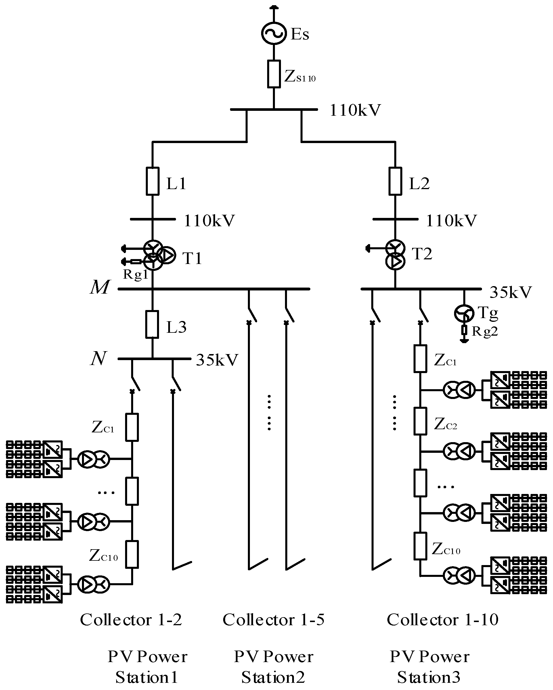
Figure 1 shows the typical topology of a grid-connected PV power station with neutral grounding resistance.
The 0.5-MW grid-connected PV inverter is widely adopted in a grid-connected PV power station, and two PV inverters are connected to the low-voltage side of a box transformer in parallel, which forms a 1-MW PV generation unit, as shown in Figure 1. Each collector line consists of 10 1-MW PV generation units, which are connected by cables (labeled Zc1–Zc10 in the figure) in the series structure and deliver to a 35-kV convergence bus (labeled N).
The capacity of a grid-connected PV power station is usually multiples of 10 MW; different capacities mean different collector lines. In general, PV stations below 30 MW will normally be sent to the nearest booster station through a 35-kV tie-line. A larger-capacity photovoltaic station, limited by the power of a 35-kV transmission line, will build the booster station on-site. The 35-kV convergence bus is directly connected to the low-pressure side of the step-up transformer. In this case, ZL35 = 0.
For the system power supply side, the system impedance in a 110-kV system is ZS110, the ratio of step-up transformer T1 is 110/35/10 kV, the connection mode is Yg/yn/d, and the neutral point on the 35-kV side is grounded by a resistance Rg. Another common connection mode of T1 is Yg/d, with a ratio of 110/35 kV; in this case, since there is no neutral point for the 35-kV side due to the triangle connection, a neutral point would be created from the grounding transformer (designated Tg) and then grounded through a resistance.
2.2. Fault-Calculation Model of Tie-Line
Given that the power-generation units are highly consistent in the same PV power station and the light intensity upon and temperature of the PV cells are substantially the same, then the following assumptions that meet the engineering requirements can be made: (1) all the parameters of the power generation units are the same, respectively; and (2) the power generated from each generation unit, at all times, are the same.
Based on the previous assumptions, when a fault occurs outside the PV station, the entire PV power station is equivalent to a large-capacity PV power supply.
It is noteworthy that ensuring the same power production is impossible. Partial shading (which is caused by clouding, dust, leaves, surrounding trees or buildings, or even different inverter operations) triggers the activation of bypass diodes, which could severely reduce PV power production [18,19,20,21]. Considering the effect of partial shading, the PV source model adds power loss coefficients at the different shading ratios and forms [18]. Table 1 shows the values.
Figure 2 illustrates the topology of a grid-connected PV power station with a fault on the 35-kV tie-line. T2 is the equivalent transformer, the impedance per unit value of T2 is equal to the box transformer, and the capacity of T2 is the sum of all box capacities in the station.
The PV power station presents the characteristic of a voltage-controlled current source, and the positive-sequence component of a short-circuit current is injected into the network [22,23]. The tie-line fault sequence network is shown in Figure 3.
In Figure 3, is the system power supply; and comprise the positive-sequence component of the voltage and short-circuit at the terminal of the PV power supply in the post-fault situation.
2.3. Fault-Calculation Model of PV-Collector Lines
When a fault occurs on the collector line inside a PV power station, the two assumptions of the tie-line model are no longer true, and the entire PV station is no longer supposed to be equivalent to a power supply. A fault model of the collector line is illustrated by Figure 4.
In Figure 4, the fault point is located on one section of cable ZCf of the PV collector line 1. The other (n − 1) collector lines are regarded as one controlled current source I(n−1)S, and the faulted collector line will be modeled in another way. Assuming that the m set of the 1-MW PV generation unit ranges from the start of the convergence bus to the faulted cable ZCf and that the n set of the 1-MW PV generation unit ranges from the faulted cable to the end of the convergence bus, they are then equivalent to an mMW controlled current source ImS and an nMW controlled current source InS (m + n = 10), respectively. The entire system is described as a multi-source network, and the collector line fault sequence network is shown in Figure 5.
In Figure 5, is the power source of the system; and and are the positive-sequence components of the voltage and short-circuit at the terminal of the (n − 1) × 10 MW PV power supply in the post-fault situation. and represent the mMW and nMW PV power supply, respectively.
When the connection mode of the step-up transformer T1 is Yg/d, as is the 35-kV side for the triangular winding, then the zero-sequence network is divided into two parts: the 35-kV side and the 110-kV side. However, the zero-sequence impedance of the grounding transformer Tg on the 35-kV side only stays in the zero-sequence network. As a consequence, the zero-sequence integrated impedance is not related to the system impedance (mode of operation) and the zero-sequence impedance of the step-up transformer.
2.4. General Nature of the Fault Model
The two above PV power-supply models are characterized by the same general nature. When the capacity of a PV power station is n × PMW (including n pairs of PMW collector lines), some adjustments must be made:
- (1)
- The maximum capacity of a PV power-supply model with a fault on the tie-line must be n × PMW.
- (2)
- The capacity of three power supplies in the collector-line model are the following: the collector line power supply without a fault is (n − 1) × PMW, and the two collector line power supplies with a fault are mMW and nMW (m + n = P).
3. Analysis of the Ground Fault
3.1. Short-Circuit Calculation Principle
Traditional power system fault analysis usually uses the nodal voltage equation method: YnUn = Jn, where Un is the nodal voltage, Yn = AYAT the nodal admittance matrix, A the correlation matrix, and Y the branch admittance matrix. Jn = AIS − AYUS is the node-injected current generated by the independent power supply, IS the independent current source, and US the independent voltage source.
For the controlled current source in the branch, the branch admittance Y must be modified, i.e., the voltage control current source (VCCS) in the kth branch, which is controlled by the voltage of the passive component Uj in the jth branch; thus, gkj should be added to the element of row k and column j in Y.
The mathematical model of a PV-controlled current source with a LVRT control strategy is given by [24] as follows:
IIDG should prioritize the provision of reactive power support after the grid fault. Considering the demand of the dynamic reactive power of IIDG [25] and the inverter capacity constraint during LVRT, the active and reactive power reference values of a PV power supply can be calculated as
where η = |US+Imax|/|UnIn| is the capacity factor of the PV inverter after the fault; US+ is the positive-sequence component of the terminal voltage of the PV power supply; and Imax = kIn is the maximum allowable current for the inverter; a typical value of k is 1.5 [26]. Sn, Un, and In are the rated capacity, voltage, and current of the PV inverter, respectively; kq is the coefficient of reactive support; and P0* and Q0* are the reference values of the active and reactive power, respectively, under normal operation.
As can be seen from Equation (1), gkj cannot simply be obtained from the complex non-linear relationship between the output current and voltage of the PV power supply. If the PV power supply is treated as an independent source, and inserted into Jn without any modification of Y and Yn, it will cause an unpredictable error in the result.
Therefore, for the fault analysis of a PV power station, the method presented in this paper builds the branch equations of the power network directly and solves them in alternating iterations.
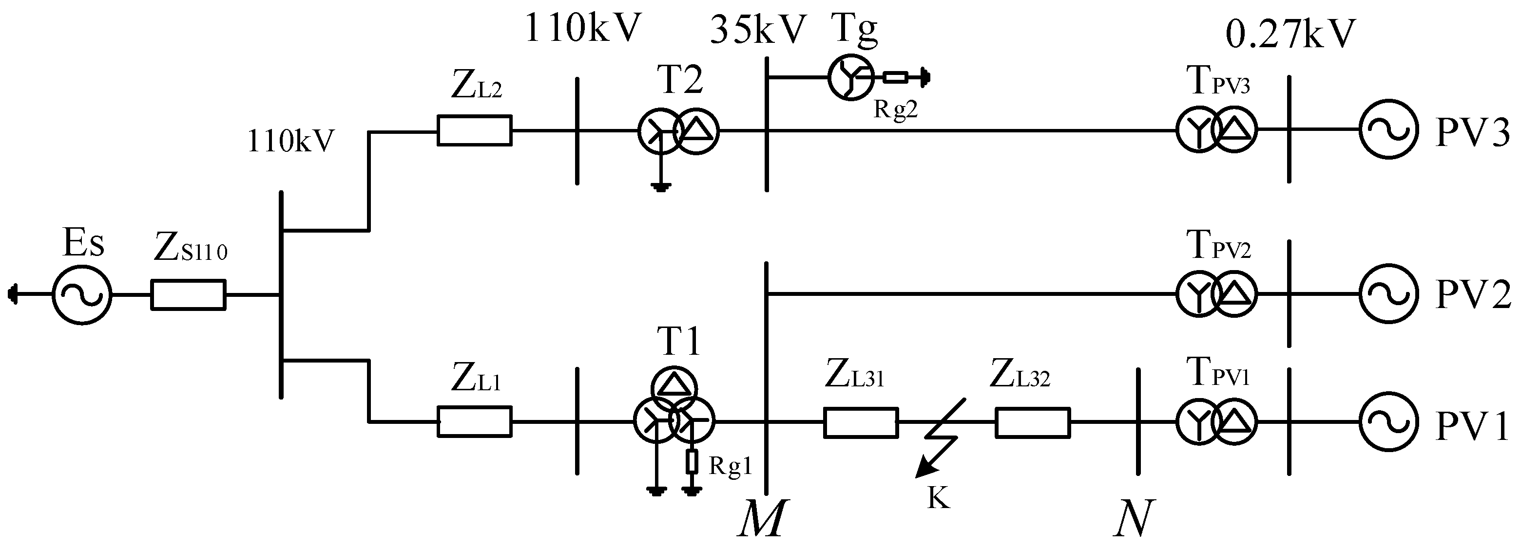
Without a loss of generality, as shown in Figure 6, the grid-connected system of multiple PV power stations is analyzed as an example.
Figure 6 shows three photovoltaic power stations (PVPSs). Through a section of the 35-kV tie-line L3, PVPS1 is sent to the step-up transformer T1; PVPS2 and PVPS3 are connected with the step-up transformer T1 and T2 on-site; and they then access the power grid through L1 and L2, respectively. The neutral point for the 35-kV side of T1 is grounded by a resistance Rg1, and the neutral point created by Tg is grounded by Rg2.
3.2. Analysis of Tie-Line Ground Fault
When the fault occurs on the tie-line L3, all PVPSs meet the two assumptions in Section 2.2, equivalent to three PV power supplies PV1, PV2, and PV3, respectively.
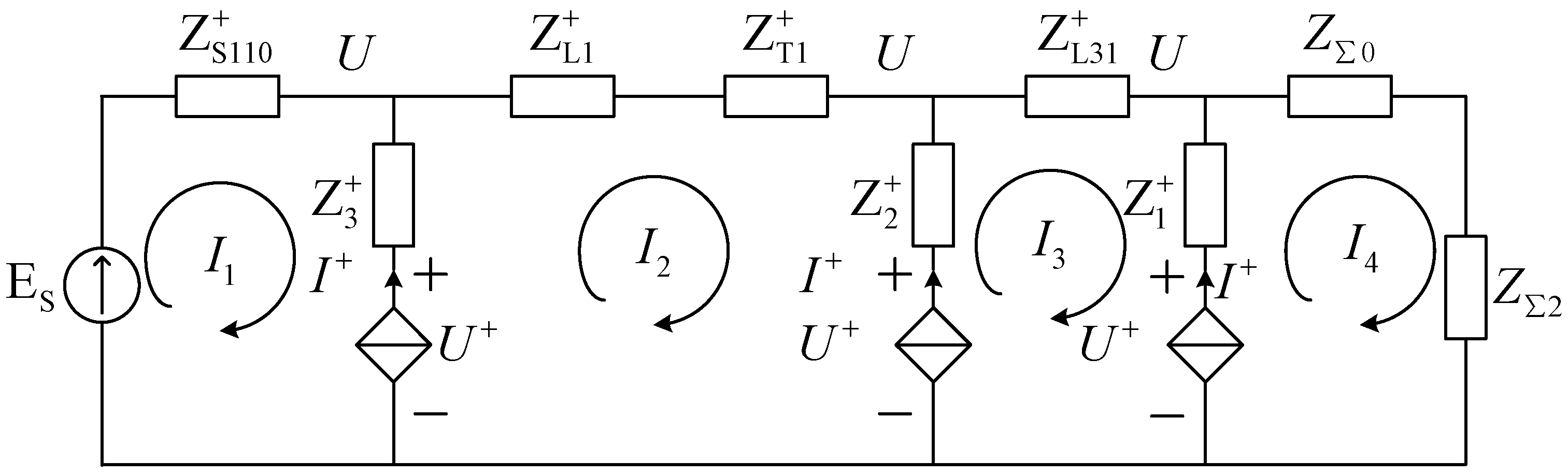
In Figure 7, TPV1, TPV2, and TPV3 are all equivalent transformers, and the equivalence principle is the same as that for T2 in Figure 2. Figure 8 shows the composite sequence network for a single-phase ground short-circuit obtained from the boundary conditions.
, , , and and are the negative- and zero-sequence integrated impedance, respectively. The loop-current equations can be obtained by the loop-current method as follows:
Equation (4) can be also derived as follows:
where , in which i denotes the number of different PV power supplies and is equal to 1, 2, and 3.
There are three PV power supplies, each of which has its own positive current, active, and reactive power equations and, combined with Equation (5), the equation for the single-phase-to ground fault is obtained. Obviously, there are 13 unknowns, , in the equations, which correspond to 13 equations and thus are solvable.
Owing to the impact of the control strategy on a PV power supply, the non-linear coupling relationship between terminal voltage and output current, resulting in non-linear equations, cannot be solved by linear analysis. The Newton–Raphson iterative method is adopted in this paper, where the convergence accuracy is 1 × 10⁻⁵.
3.3. Analysis of Collector-Line Ground Fault
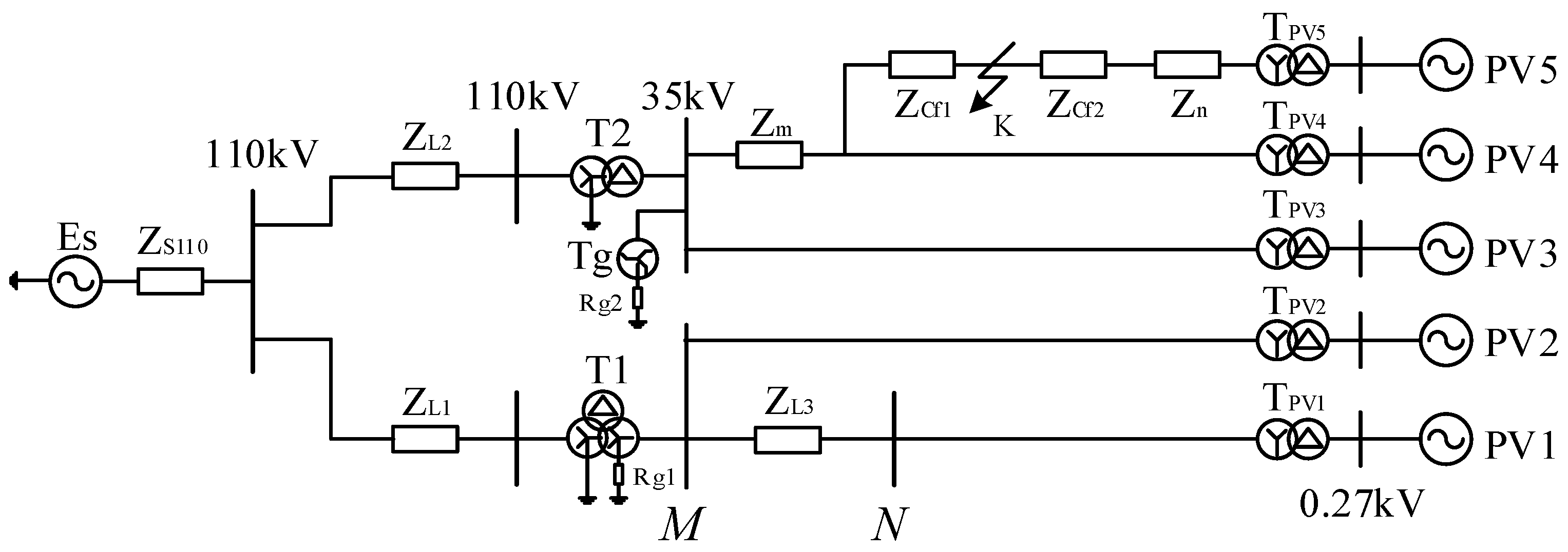
When a fault occurs on the collector line in the PVPS3 station, PVPS1 and PVPS2 also meet the two assumptions, but PVPS3 is equivalent to three PV sources, as shown in Figure 9.
The composite sequence network for a two-phase ground short-circuit obtained from the boundary conditions is shown in Figure 10.
, , , , and , and the equations are obtained as follows:
where , in which , and i is equal to 1, 2, 3, 4, and 5. In addition, .
Combined with the positive current, active and reactive power equations of five PV power supplies, the 21 equations correspond to the 21 unknowns, , and thus are solvable.
4. Analysis of the Fault Characteristic and Impact on Protection
Based on the ground-fault analysis method, this section discusses further the general rule of the short-circuit current characteristic with the fault type, the photovoltaic capacity, the fault location, the grounding resistance of the neutral point, and the possible influence on grid protective actions.
To indicate the analytical result clearly, a case study of the typical network, shown in Figure 6, is required. The control parameters are kq = 1, P0* = 0.8 p.u., and Q0* = 0.6 p.u. [24], and the other parameters are given in the Appendix A.
4.1. Fault Characteristic of the PV Power Supply
Case 1: The fault occurs at the end of L3 (bus N).
Figure 11 shows the change of the PV source output current values with the variation of PV1 capacity (Sn PV1) and Rg1 under the condition that the ground fault occurs at the L3 end.
The capacity range of PVPS1 is 10–30 MW, that of PVPS2 and PVPS3 is 10–200 MW, and the range of Rg1 and Rg2 is 10–200 Ω.
Figure 11a indicates that the main effect of the PV1 output current |IPV1| is from the capacity of the PV1 power supply. As the capacity of the PV1 power supply, Sn PV1, becomes smaller, |IPV1| decreases dramatically. In terms of ground-fault type, the output current with a two-phase grounding fault is larger than that with a single-phase grounding fault, because the terminal voltage of the PV power supply with two-phase decreases more substantially. The influence of neutral grounding resistance on the output current of a PV power supply with single-phase grounding is larger than that with two-phase grounding, which reflects the difference between a series fault and a parallel fault.
Figure 11b–d shows that the pre-unit output current is always controlled to be within the allowable range (1.5 times the rated current) under the inverter LVRT control strategy, whether a single-phase or two-phase grounding fault occurs. It is also noted that the output pre-unit current of different PV power supplies decreases gradually with the increase of Sn PV1, which indicates that each PV power supply in the grid-connected system upon an increase of the total capacity of the PV source could provide more reactive power support when the fault voltage drops in the grid (LVRT is more capable).
Located at the far end of the fault, the changes in fault conditions hardly affect the output current of the PV source, especially across the transformer; as with PV3, the change of each dimension is within 4‰. By contrast, the parameter change greatly affects the PV sources that all exhibit the same change trend. In general, the closer the PV source is to the point of the grounding fault, the greater the effect of the fault conditions on the fault output current, and the more likely the fault current will be close to the maximum output current of the inverter.
Considering the effect of partial shading on PV1, the PV1 output current values of the shading ratio are shown in Table 2. (Sn PV1 = 30 MW, Sn PV2 = 50 MW, Sn PV3 = 100 MW, Rg1 = 20 Ω).
As seen from Table 2, PV1 output current value |IPV1| reaches maximum without shading, and this value is decreased with the increase in shading ratio. Based on this table, |IPV1| decreases from 700.07 A to 12.41 A. The shading ratio and shading shape have a significant effect on the output current of PV sources.
Case 2: The fault occurs at the end of one collector line in the PVPS3 station.
When a ground fault occurs at the end of the collector line in the PVPS3 station, the change characteristics of the different PV power supply output currents with respect to the capacity of the PV2 power supply, (Sn PV2), and Rg2 can be obtained through the simulation example.
The PV source current characteristics of the collector fault are consistent with the fault of the tie-line. With the increase of PV2 power capacity Sn PV2, the total capacity of the PV source increases the fault ride-through ability of all the PV sources in the grid-connected system. Therefore, the fault output current per-unit value of PV1 to PV5 is slightly reduced.
Similarly, the difference between single-phase and two-phase faults of the PVs, which are far from the point of a grounding fault, is quite small. Moreover, the PVs near the fault point, especially the two-phase fault currents of PV4 and PV5 on the fault collector line, are close to the maximum allowable output current.
4.2. Fault Characteristics of Zero-Sequence Current
Table 3 shows the zero sequence current values with the variation of shading ratio and shading shape under the condition that the ground fault occurs at the L3 end.
Table 3 shows that the zero-sequence current is almost unaffected by the partial shading, since that PV power supply cannot directly output a zero-sequence current. Minor changes come from the variation of integrated electromotive force caused by a PV source under the different shading ratios.
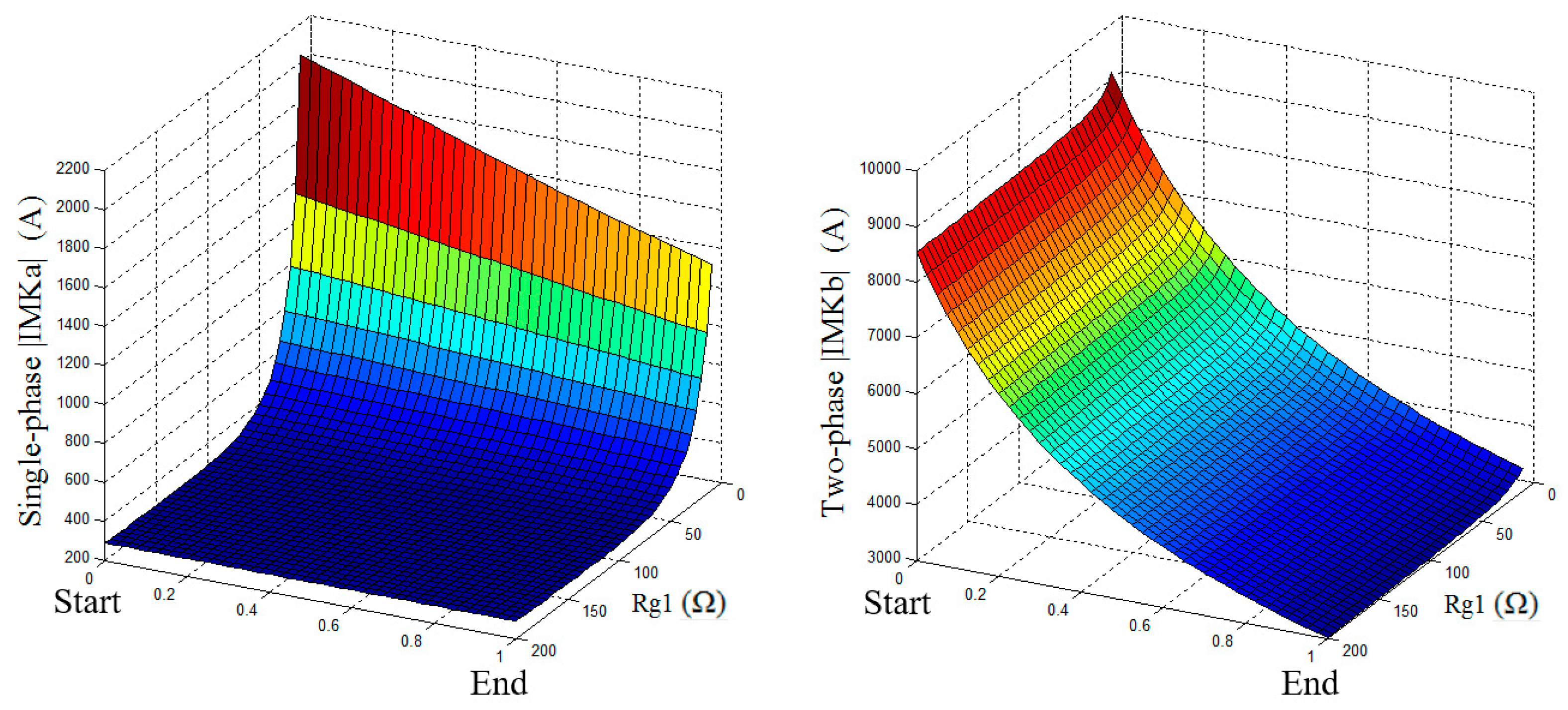
As the fault location moves from the start (bus M) to end (bus N) of the tie-line L3, the change characteristics of the zero-sequence current with a different fault position and the neutral point grounding resistance Rg1 is analyzed in Figure 12.
The zero-sequence currents with the single-phase grounding fault and the two-phase grounding fault [27] are calculated as
where consists of 3Rg1, Rg1 (10,200), so is larger than , and when Rg1 is large enough, and ; this law is also reflected in Figure 12.
Figure 12a shows that the zero-sequence current decreases as Rg1 increases. When Rg1 is small, as the fault location moves from the start to the end of L3, |I0| decreases, while Rg1 increases, and the change speed of |I0| is slowed gradually with the same movement of the fault location. Figure 12b is drawn in order to clearly describe this phenomenon: When Rg1 = 10 Ω, the curve of |I0| decreases significantly; when Rg1 = 30 Ω, the curve decreases very slowly, and is almost horizontal when Rg1 = 50 Ω; when Rg1 = 100 Ω, the curve of |I0| increases slightly. The data are shown in Table 4.
It can be seen clearly that when Rg1 = 10 Ω, with the fault moving from the start to the end of the tie-line L3, the variation trend of the zero-sequence current is |I0 Start|>|I0 Middle|>|I0 End|. When Rg1 = 100 or 200 Ω, |I0 Start|<|I0 Middle|<|I0 End|. The following specific analysis reveals the reasons why the zero-sequence current changes bidirectionally under different Rg1 values.
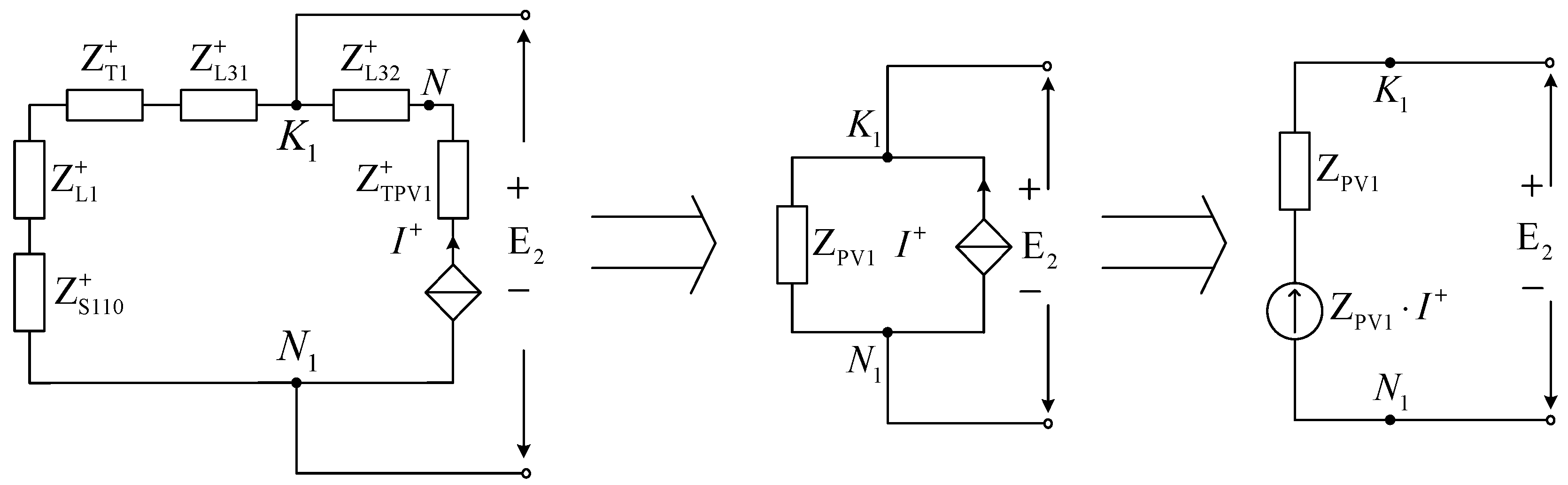
When a fault occurs in the grid, the voltage at the point of common coupling (PCC) of the PV power supply decreases. The inverter combines the instantaneous network fault state, the security constraints, and the LVRT control strategy to adjust the output current in order to track the reference current. The fault response speed of the inverter is within milliseconds, and the fault steady state is achieved. At t0+ time, the system power supply is considered to be a constant voltage source, and the PV power supply reaches a relative balance; thus, it is considered a constant current source as well. Then, in (7) is the integrated equivalent power supply of the system power and PV power supplies shown in Figure 13.
Using the superposition theorem, at t0+ time, the equivalent power supplies , , , and with the fault on the K1 point are obtained by assuming that the system power and PV sources work separately; then, .
The system power supply is considered a constant voltage source, so , and the equivalent of a PV current source is shown in Figure 14.
As shown in Figure 14, . For the same reason, , , where , , and . Thus, the zero-sequence current with the single-phase grounding fault can be expressed as
As the fault location moves on the tie-line L3, only (containing ) and change in (8). Assuming that is constant, when the fault location is at the start, middle, and end of L3, the is , , and , respectively:
where and . When Rg1 changes, three conclusions can be reached:
(a) If Rg1 is small, , and then
that is, .
(b) If Rg1 increases gradually to , , and at this point the resistance value of Rg1 is called Rg1balance.
(c) If Rg1 is large, , and then .
In the following, the variation of with respect to the fault location is further analyzed. As the fault location approaches the end of L3, increases and decrease. Under the same Rg1 conditions, then,
In other words, when the condition of the variation of is added, the phenomenon of zero-sequence current reversal appears earlier.
The neutral grounding resistance mainly affects the zero-sequence current, which decreases with increasing resistance value. The PV current source will increase the system’s integrated electromotive force; in general, the integration of a PV power supply facilitates the increase of the zero-sequence current. The larger the capacity of the PV power supply, the more obvious the effect on the increase of the zero-sequence current. This may result in a malfunction of the zero-sequence protection device and in a loss of selectivity.
Affected by the neutral grounding resistance, the zero-sequence current exhibits a bidirectional change characteristic with respect to the fault location, and this kind of proportional relation may lead to a malfunction of the zero-sequence protection set by the traditional method. Meanwhile, when the neutral grounding resistance is large, the curve of the zero-sequence current varies gently with respect to the fault position, which leads to a loss of protection sensitivity.
4.3. Fault Characteristics of the Phase Current
When a ground fault occurs at different locations on the tie-line L3, the fault characteristics of the phase current are as shown in Figure 15.
Figure 15 shows that the fault phase current through the tie-line will gradually decrease with the fault location from the start to the end of L3, whether a single-phase or two-phase grounding fault occurs.
Simultaneously, it can clearly be seen from the figure that the phase current with a two-phase grounding fault changes with the position of the fault, and is less affected by Rg1. Obviously, however, the phase current with a single-phase grounding fault changes only if Rg1 is small.
After analyzing the reason for the previous scenario, the phase current with a single-phase grounding fault [27] is
From (11), when Rg1 is small, the zero- and the positive-sequence integrated impedance are still the same order of magnitude, so obviously the change of the line impedance caused by the movement of the fault location can also change the fault-phase current.
However, when Rg1 is large, , so the line impedance caused by the fault location movement has less impact on the phase current.
The phase current with a two-phase grounding fault [27] is
When Rg1 is large, , and then
Therefore, the movement of the fault position always has a great influence on the fault phase current with a two-phase grounding fault regardless of the value of Rg1.
The neutral grounding resistance hardly affects the fault phase current with a two-phase grounding, and its change characteristic is similar to the system with ungrounded neutral resistance. As the fault location moves from the start to the end of the line, the phase current decreases gradually, which can eliminate the two-phase grounding fault using the traditional phase-to-phase current protection.
5. Conclusions
Based on the equivalent fault model of a PV power supply using a LVRT control strategy, this paper conducts research on a grid-connected PV power station with neutral grounding resistance. By considering the general rule of two types of lines (system tie-line and station collector line), it presents a comprehensive fault analysis model of multiple grid-connected PV power stations and the mathematical solution. From the perspective of the zero-sequence current characteristics and fault network, the utility of the proposed model and method is then proved by a simulation case study, especially under the exclusive operating mode of grid-connected PV stations with neutral grounding resistance. The proposed fault model features simple implementation for different grid topologies, PV station capacities, and fault types; and the results of simulations under different scenarios show general rules of short-circuit currents and the potential impact on grid protection with respect to the system parameters, especially the neutral grounding resistance. This can provide abundant information for engineers to gain a better understanding of the fault responses of PVs and to design improved protection for the stable operation of grid-connected PV systems.
Acknowledgments
This work was supported in part by the National Natural Science Foundation of China under Grant No. 51577018.
Author Contributions
All authors (Z.L., J.L., Y.Z., and W.J.) contributed to compiling the manuscript in its current state. Their contributions included a detailed survey of the literature and state-of-the-art scenarios which were essential for the completion of this paper. Z.L. wrote the paper.
Conflicts of Interest
The authors declare no conflict of interest.
Appendix A.
The grid-connected system parameters are as follows:
- (1)
- The short-circuit capacity of a 110-kV system is 3000 MVA.
- (2)
- The parameters of the transformers are as follows:
- (a)
- The capacity of the transformers varies with the PV source.
- (b)
- T1 parameters: VI/VII/VIII (Yg/yn/d) = 110/35/10 kV; UKI = 10.75%, UKII = 0, and UKIII = 6.75%.
- (c)
- T2 parameters: VI/VII (Yg/d) = 110/35 kV; UK = 10.75%.
- (d)
- All the box-type transformers have the same parameters: Sn = 1 MVA, VI/VII (Y/d) = 35/0.27 kV, and UK = 6%.
- (3)
- The line lengths and impedance (per kilometer) are as follows:
- (a)
- All the pre-unit parameters of the positive and negative sequences are the same, and the pre-unit parameters of the zero sequence are 3 times those of the positive and negative sequences.
- (b)
- L1 = 9 km and L2 = 6 km, which uses LGJ-2 × 400, and the positive sequence impedance is 0.08 + j0.414 Ω/km.
- (c)
- L3 = 10 km, which uses LGJ-240, and the positive sequence impedance is 0.132 + j0.386 Ω/km.
- (4)
- The cable length of each collector line is 3 km, which uses YJV22-3 × 95 mm, and the positive sequence impedance is 0.196 + j0.129 Ω/km.
References
- Guerrero, J.M.; Blaabjerg, F.; Zhelev, T.; Hemmes, K.; Monmasson, E.; Jemei, S.; Comech, M.P.; Granadino, R.; Frau, J.I. Distributed generation: Toward a new energy paradigm. IEEE Ind. Electron. Mag. 2010, 4, 52–64. [Google Scholar] [CrossRef]
- Castilla, M.; Miret, J.; Sosa, J.L.; Matas, J.; de Vicuña, L.G. Grid-fault control scheme for three-phase photovoltaic inverters with adjustable power quality characteristics. IEEE Trans. Power Electron. 2010, 25, 2930–2940. [Google Scholar] [CrossRef]
- Miret, J.; Castilla, M.; Camacho, A.; de Vicuña, L.G.; Matas, J. Control scheme for photovoltaic three-phase inverters to minimize peak currents during unbalanced grid-voltage sags. IEEE Trans. Power Electron. 2012, 27, 4262–4271. [Google Scholar] [CrossRef]
- Hooshyar, H.; Baran, M.E. Fault analysis on distribution feeders with high penetration of PV systems. IEEE Trans. Power Syst. 2013, 28, 2890–2896. [Google Scholar] [CrossRef]
- State Grid Corporation of China (SGCC). Q/GDW 1617-2015 Technical Rule for Connecting Photovoltaic Power Station to Power Grid; State Grid Corporation of China: Beijing, China, 2015. [Google Scholar]
- Nimpitiwan, N.; Heydt, G.T.; Ayyanar, R.; Suryanarayanan, S. Fault current contribution from synchronous machine and inverter based distributed generators. IEEE Trans. Power Deliv. 2007, 22, 634–641. [Google Scholar] [CrossRef]
- Nuutinen, P.; Peltoniemi, P.; Silventoinen, P. Short-circuit protection in a converter-fed low-voltage distribution network. IEEE Trans. Power Electron. 2013, 28, 1587–1597. [Google Scholar] [CrossRef]
- Ustun, T.S.; Ozansoy, C.; Ustun, A. Fault current coefficient and time delay assignment for microgrid protection system with central protection unit. IEEE Trans. Power Syst. 2013, 28, 598–606. [Google Scholar] [CrossRef]
- Haj-ahmed, M.A.; Illindala, M.S. The influence of inverter-based DGs and their controllers on distribution network protection. IEEE Trans. Ind. Appl. 2014, 50, 2928–2937. [Google Scholar] [CrossRef]
- Pan, G.; Zeng, D.; Wang, G.; Zhu, G.L.; Li, H.F. Fault analysis on distribution network with inverter interfaced distributed generations based on PQ control strategy. Proc. CSEE 2014, 34, 555–561. [Google Scholar]
- Baran, M.E.; El-Markaby, I. Fault analysis on distribution feeders with distributed generators. IEEE Trans. Power Syst. 2005, 20, 1757–1764. [Google Scholar] [CrossRef]
- Wu, Z.; Wang, G.; Li, H.; Pan, G.; Gao, X. Analysis on the distribution network with distributed generators under phase-to-phase short-circuit faults. Proc. CSEE 2013, 33, 130–136. [Google Scholar] [CrossRef]
- Camacho, A.; Castilla, M.; Miret, J.; Vasquez, J.C.; Alarcón-Gallo, E. Flexible voltage support control for three-phase distributed generation inverters under grid fault. IEEE Trans. Ind. Electron. 2013, 60, 1429–1441. [Google Scholar] [CrossRef]
- Guo, W.M.; Mu, L.H.; Zhang, X. Fault Models of Inverter-Interfaced Distributed Generators within a Low-Voltage Microgrid. IEEE Trans. Power Deliv. 2017, 32, 453–461. [Google Scholar] [CrossRef]
- Camacho, A.; Castilla, M.; Miret, J.; Borrell, A.; de Vicuña, L.G. Active and reactive power strategies with peak current limitation for distributed generation inverters during unbalanced grid faults. IEEE Trans. Ind. Electron. 2015, 62, 1515–1525. [Google Scholar] [CrossRef]
- Guo, X.; Zhang, X.; Wang, B.; Wu, W.; Guerrero, J.M. Asymmetrical grid fault ride-through strategy of three-phase grid-connected inverter considering network impedance impact in low-voltage grid. IEEE Trans. Power Electron. 2014, 29, 1064–1068. [Google Scholar] [CrossRef]
- Shuai, Z.; Shen, C.; Yin, X.; Liu, X.; Shen, J. Fault analysis of inverter-interfaced distributed generators with different control schemes. IEEE Trans. Power Deliv. 2017, 10, 1–13. [Google Scholar] [CrossRef]
- Bayrak, F.; Erturk, G.; Oztop, H.F. Effects of partial shading on energy and exergy efficiencies for photovoltaic panels. J. Clean. Prod. 2017, 164, 58–69. [Google Scholar] [CrossRef]
- Das, S.K.; Verma, D.; Nema, S.; Nema, R.K. Shading mitigation techniques: State-of-the-art in photovoltaic applications. Renew. Sustain. Energy Rev. 2017, 78, 369–390. [Google Scholar] [CrossRef]
- Bana, S.; Saini, R.P. Experimental investigation on power output of different photovoltaic array configurations under uniform and partial shading scenarios. Energy 2017, 127, 438–453. [Google Scholar] [CrossRef]
- Bastidas-Rodríguez, J.D.; Trejos-Grisales, L.A.; González-Montoya, D.; Ramos-Paja, C.A.; Petrone, G.; Spagnuolo, G. General modeling procedure for photovoltaic arrays. Electr. Power Syst. Res. 2018, 155, 67–79. [Google Scholar] [CrossRef]
- Wang, F.; Duarte, J.L.; Hendrix, M.A. Pliant active and reactive power control for grid-interactive converters under unbalanced voltage dips. IEEE Trans. Power Electron. 2011, 26, 1511–1521. [Google Scholar] [CrossRef]
- Peng, F.Z.; Lai, J.S. Generalized instantaneous reactive power theory for three-phase power systems. IEEE Trans. Instrum. Meas. 1996, 45, 293–297. [Google Scholar] [CrossRef]
- Wang, Q.; Zhou, N.; Ye, L. Fault analysis for distribution networks with current-controlled three-phase inverter-interfaced distributed generators. IEEE Trans. Power Deliv. 2015, 30, 1532–1542. [Google Scholar] [CrossRef]
- Bae, Y.; Vu, T.K.; Kim, R.Y. Implemental control strategy for grid stabilization of grid-connected PV system based on German grid code in symmetrical low-to-medium voltage network. IEEE Trans. Energy Convers. 2013, 28, 619–631. [Google Scholar] [CrossRef]
- State Grid Corporation of China (SGCC). GB/T 32826-2016 Guide for Modeling Photovoltaic Power System; Standardization Administration of China: Beijing, China, 2016.
- Grainger, J.; Stevenson, W. Power System Analysis; McGraw-Hill: New York, NY, USA, 1994; pp. 470–527. [Google Scholar]
Figure 1.
Grid-connected photovoltaic (PV) station with neutral grounding resistance.
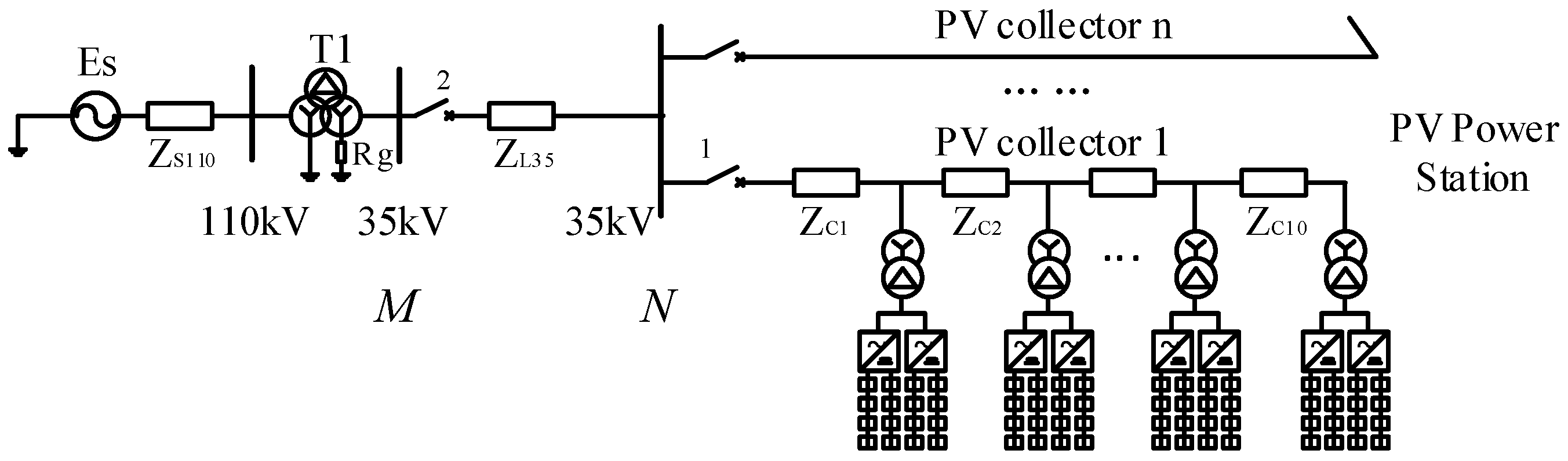
Figure 2.
The equivalent circuit diagram with the fault on the tie-line.

Figure 3.
Fault sequence network for the fault on the tie-line.
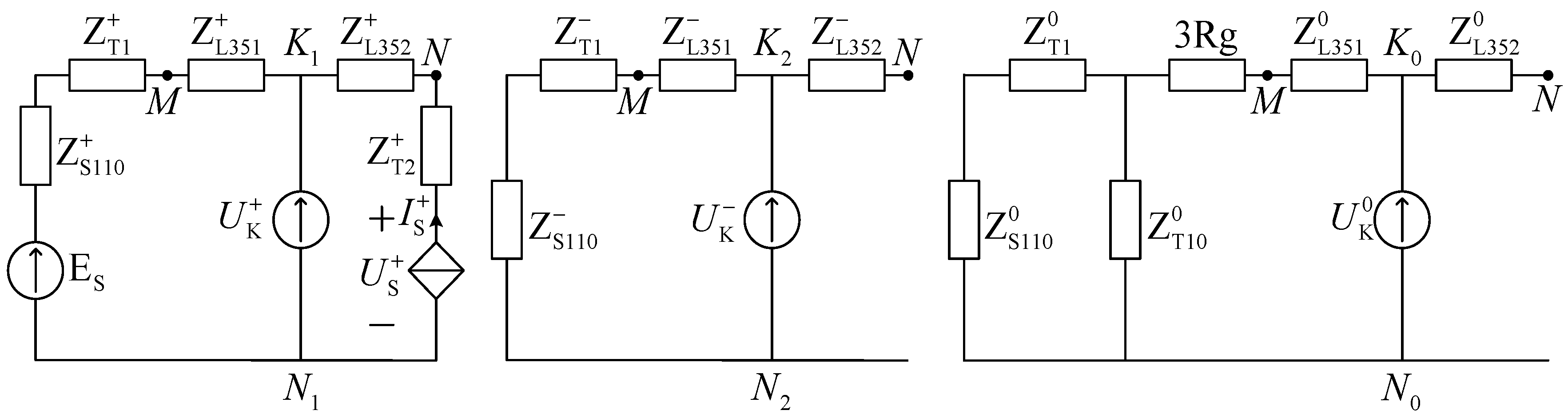
Figure 4.
Equivalent circuit for the fault on the collector line.

Figure 5.
Fault sequence network for the fault on the collector line.
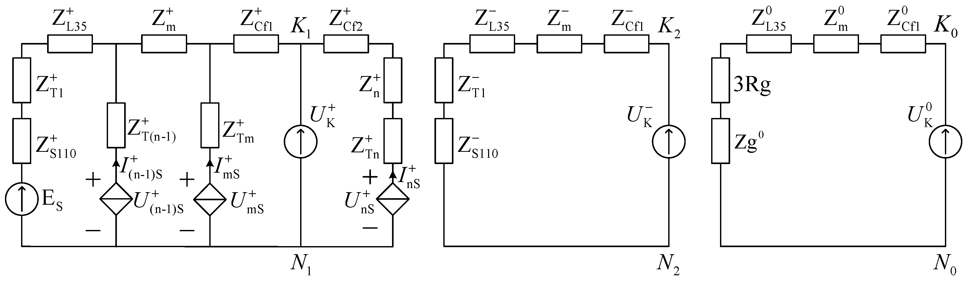
Figure 6.
Grid-connected system of multiple PV power stations.

Figure 7.
Equivalent circuit diagram with the fault on the tie-line L3.

Figure 8.
Composite sequence network for a single-phase ground short-circuit on L3.

Figure 9.
Equivalent circuit for the fault on the collector line in photovoltaic power station (PVPS) 3.
Figure 9.
Equivalent circuit for the fault on the collector line in photovoltaic power station (PVPS) 3.

Figure 10.
Complex sequence network of two-phase ground fault on the collector line in PVPS3.
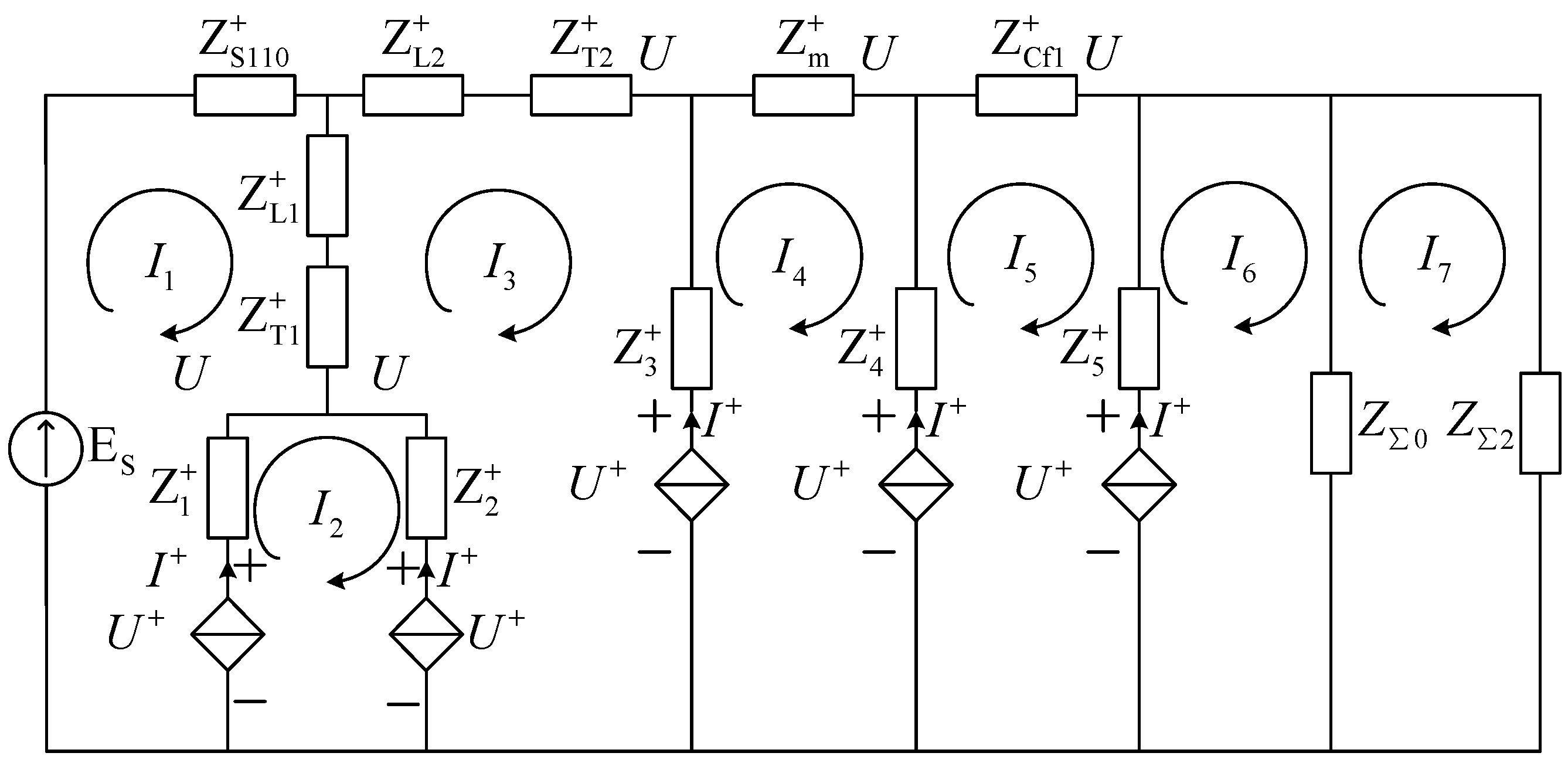
Figure 11.
Characteristic of the PV power supply output current with the ground fault at the end of L3. (a) Output current of PV1, |IPV1|; (b) output current per-unit of PV1, IPV1.PU; (c) output current per-unit of PV2, IPV2.PU; (d) output current per-unit of PV3, IPV3.PU.
Figure 11.
Characteristic of the PV power supply output current with the ground fault at the end of L3. (a) Output current of PV1, |IPV1|; (b) output current per-unit of PV1, IPV1.PU; (c) output current per-unit of PV2, IPV2.PU; (d) output current per-unit of PV3, IPV3.PU.
Figure 12.
Characteristics of the zero-sequence current |I0| with respect to the fault location and Rg1. (a) Change surface of the zero-sequence current |I0| with respect to the fault location and Rg1; (b) change curve of the zero-sequence current |I0| with respect to the fault location at the different Rg1 condition.

Figure 13.
Positive sequence network of the equivalent integrated power supply.

Figure 14.
Equivalent network of PV1 current source.

Figure 15.
Change characteristic of the fault phase current with respect to fault location and Rg1.


Table 1.
Power loss coefficient values of shading ratio.
| SR (Shading Ratio) | Power Loss Coefficient (%) | ||
|---|---|---|---|
| Single-Cell | Horizontal | Vertical | |
| 0.00 | 0.00 | 0.00 | 0.00 |
| 0.25 | 9.06 | 34.53 | 16.99 |
| 0.50 | 65.88 | 75.97 | 18.85 |
| 0.75 | 66.38 | 92.96 | 61.88 |
| 1.00 | 69.22 | 99.98 | 66.93 |
Table 2.
PV1 output current values of partial shading.
| Fault Type | SR (Shading Ratio) | PV1 Output Current Values |IPV1| (A) | ||
|---|---|---|---|---|
| Single-Cell | Horizontal | Vertical | ||
| Single phase to ground | 0.00 | 503.11 | 503.11 | 503.11 |
| 0.25 | 455.75 | 334.72 | 423.85 | |
| 0.50 | 176.16 | 123.81 | 415.83 | |
| 0.75 | 175.62 | 35.83 | 201.16 | |
| 1.00 | 158.40 | 9.02 | 175.32 | |
| Double phase to ground | 0.00 | 700.07 | 700.07 | 700.07 |
| 0.25 | 632.46 | 461.17 | 587.10 | |
| 0.50 | 243.68 | 168.26 | 575.72 | |
| 0.75 | 241.53 | 48.39 | 274.80 | |
| 1.00 | 215.76 | 12.41 | 239.32 | |
Table 3.
Zero-sequence current values of partial shading.
| Fault Type | SR (Shading Ratio) | Zero-Sequence Current Values |I0| (A) | ||
|---|---|---|---|---|
| Single-Cell | Horizontal | Vertical | ||
| Single phase to ground | 0.00 | 353.37 | 353.37 | 353.37 |
| 0.25 | 350.17 | 341.89 | 348.00 | |
| 0.50 | 331.02 | 327.05 | 347.45 | |
| 0.75 | 330.83 | 320.64 | 332.57 | |
| 1.00 | 329.53 | 318.64 | 330.66 | |
| Double phase to ground | 0.00 | 198.62 | 198.62 | 198.62 |
| 0.25 | 196.36 | 190.59 | 194.83 | |
| 0.50 | 183.32 | 180.61 | 194.45 | |
| 0.75 | 183.10 | 176.46 | 184.26 | |
| 1.00 | 182.24 | 175.20 | 183.03 | |
Table 4.
Zero-sequence current values with the different fault location on the tie-line L3.
| Fault Type | Rg1 (Ω) | Zero Sequence Current with Different Fault Locations |I0| (A) | ||
|---|---|---|---|---|
| Start | Middle | End | ||
| Single phase to ground | 10 | 739.81 | 641.14 | 550.60 |
| 30 | 254.61 | 250.24 | 244.33 | |
| 50 | 153.93 | 153.94 | 153.95 | |
| 100 | 77.02 | 78.30 | 79.49 | |
| 200 | 38.57 | 39.45 | 40.32 | |
| Double phase to ground | 10 | 395.13 | 365.69 | 334.46 |
| 30 | 132.51 | 132.37 | 132.23 | |
| 50 | 79.58 | 80.51 | 81.71 | |
| 100 | 39.82 | 40.63 | 41.64 | |
| 200 | 19.91 | 20.41 | 21.00 | |
© 2017 by the authors. Licensee MDPI, Basel, Switzerland. This article is an open access article distributed under the terms and conditions of the Creative Commons Attribution (CC BY) license (http://creativecommons.org/licenses/by/4.0/).
Share and Cite
MDPI and ACS Style
Li, Z.; Lu, J.; Zhu, Y.; Jiang, W. Ground-Fault Characteristic Analysis of Grid-Connected Photovoltaic Stations with Neutral Grounding Resistance. Energies 2017, 10, 1910. https://doi.org/10.3390/en10111910
AMA Style
Li Z, Lu J, Zhu Y, Jiang W. Ground-Fault Characteristic Analysis of Grid-Connected Photovoltaic Stations with Neutral Grounding Resistance. Energies. 2017; 10(11):1910. https://doi.org/10.3390/en10111910
Chicago/Turabian StyleLi, Zheng, Jiping Lu, Ya Zhu, and Wang Jiang. 2017. "Ground-Fault Characteristic Analysis of Grid-Connected Photovoltaic Stations with Neutral Grounding Resistance" Energies 10, no. 11: 1910. https://doi.org/10.3390/en10111910
Note that from the first issue of 2016, this journal uses article numbers instead of page numbers. See further details here.