Assessing the Quality of Natural Gas Consumption Forecasting: An Application to the Italian Residential Sector


Dipartimento di Ingegneria meccanica, energetica, gestionale e dei trasporti (DIME), University of Genoa, via All’Opera Pia 15 A, 16145 Genoa, Italy
*
Author to whom correspondence should be addressed.
Energies 2017, 10(11), 1879; https://doi.org/10.3390/en10111879
Submission received: 23 October 2017
/
Revised: 10 November 2017
/
Accepted: 13 November 2017
/
Published: 16 November 2017
Abstract
:(1) Background: The present paper aims at estimating the quality of the forecasts obtained by using one equation models. In particular, the focus is on the effect that the explanatory variables have on the forecasted quantity. The analysis is performed on the long term natural gas consumption in the Italian residential sector, but the same methodology can be applied to other contexts; (2) Methods: Different ex ante knowledge scenarios are built by associating different levels of confidence to the same set of explanatory variables. Forecasting results, coming from a standard regression algorithm and confirmed by a Kalman filter, are analyzed by means of covariance matrix propagation to assess the quality of the provided estimates; (3) Results: The outcomes show that one-equation models are very sensitive to the quality of the explanatory variables, therefore their erroneous estimation may have a relevant detrimental effect on the predictive accuracy of the model; (4) Conclusions: The overall ex ante forecasting accuracy of an example of one equation model is assessed. It has emerged that long-term forecasts need particular attention when the covered time horizon spans over decades. The information contained in the present paper is of interest for energy planners, supply network managers and policy makers in order to support their decisions.
1. Introduction and Literature Review
Primary energy consumption forecasting is of fundamental importance since it is essential in a multitude of different sectors and activities. A simple example is represented by companies which sell energy, as they need to know the demand of their customers in order to organize their supply chains. The estimation of future consumption of primary energy is a key element also in case of energy infrastructure planning and construction, such as pipelines, storages and so on, because the expected consumptions are the main input for their evaluation and design. Other areas of application are the elaboration of energy policies, the study of demand side management strategies, the analysis of energy markets and many other fields [1].
As one can notice, the subject is broad and different approaches have been developed attempting to create accurate models representing the evolution of energy consumption in the future. These models have been applied to predict the demand of different energy sources, such as electricity, natural gas, coal and others, with different time horizons, i.e., short, medium and long term predictions.
Short term predictions are usually utilized to support market operations, while long term predictions are generally employed to support strategic decisions, whereas medium term estimates can be used for both, depending on the specific sector of application.
In energy demand modeling, there are usually two main approaches: “top down” and “bottom up” modeling. The bottom-up approach is mostly used when there is a detailed level of information, based on equipment load factor, efficiencies and usage [2]. For example, this approach is often utilized in the simulation of power markets [3]. Top down methods are often used when available information on equipment or appliance stocks is limited [2]. These methods are typically applied to forecast long term energy consumption [4,5].
Most of the literature available on the long term forecasting of energy consumption is devoted to the electricity or to global energy consumption, while the specific sources of primary energy have deserved less consideration [6], probably due to the difficulty in getting data to develop the analysis.
During the last 20 years, an increase of natural gas consumption has been regularly detected year by year. In light of this, different authors decided to investigate on the analysis and forecasting of natural gas consumptions by using different approaches and methodologies.
Huntington [7] proposed a statistical model of industrial US natural gas consumption based upon historical data from the 1958–2003 time period. The model specifically addresses interfuel substitution possibilities and changes in the industrial economic base. His idea was to provide a valuable input for larger and more complex models. Sailor and Muñoz [8] developed a technique to assess the relation between electricity and natural gas consumption and climate at regional scales. The advantages and disadvantages of using primitive (i.e., temperature) and derived variables (i.e., heating degree days) are discussed in that paper.
Potočnik and coworkers [9] tested different static and adaptive models for short-term natural gas consumption. From the investigation, a clear improvement of the prediction performance emerges when the adaptive variant of the models is utilized if the forecasting is applied to the distribution company, while performances are not affected when dealing with individual house consumption. Iranmanesh [10] proposed a hybrid approach for long-term demand forecasting based on the neuro-fuzzy model. The approach is implemented in three case studies for the prediction of long-term gasoline, crude oil and natural gas demand in the United States.
Similarly, Bianco et al. [11] proposed a long term top down model to forecast natural gas consumption in the Italian non-residential sector. A model is developed relating historical consumption, economic growth and climatic data, in order to perform an analysis under different scenarios of the explaining variables. Moreover, Soldo et al. [12] investigated the effect of solar radiation on forecasting residential natural gas consumption. Solar radiation impact is tested against natural gas consumption data from a model house and from measurement taken from a distribution company. Furthermore, Lu et al. [13] proposed a novel statistical method to predict energy consumption in the building sector. Their work takes into account the stochastic nature of weather conditions, energy consumption and loads.
Other authors [14] have proposed a new study based on the grey forecasting methodology. In particular, they suggested the utilization of grey Verhulst model and the nonlinear grey Bernoulli model to forecast long term natural gas consumption in China. Also, Shaikh and Ji [15] investigated on the prediction of natural gas consumption in China. They suggest the application of a logistic model coupled with the Levenberg-Marquardt Algorithm for the estimation of the model parameters. Furthermore, Szoplik [16] analyzes the application of an artificial neural network with hourly resolution for the estimation of the natural gas demand. The model is intended for the optimization of the operation of the natural gas network.
Recently, Soldo [17] presented a review on the literature dealing with forecasting of natural gas consumption, where he reported the state of the art on this subject. He examined many papers and grouped them by using different criteria, among which the forecasting technique utilized.
In the reviewed literature, the subject “forecasting accuracy” is tackled from the point of view of the “ex post comparison” of measured data against the forecasted data obtained by using the model to be tested. This can be easily done in case of short-term forecasting while very-long-term projections ask for “ex ante” methods that can provide an estimation of the “expected forecasting quality” by using covariance propagation techniques.
Three factors drive the value of the accuracy: the first is the intrinsic volatility of the phenomenon to be investigated and its sensitivity to the interconnected explanatory variables which control its time evolution; the second driving factor is the level of knowledge about the future behavior of the explanatory variables since also a perfect model is completely useless if it is driven by uncertain variables and the third is the model itself, i.e., a bad model rarely leads to good estimates.
The present study is focused on the quality assessment of “one equation” long-term forecasting models since this approach is frequently applied to the prediction of both electricity [4,18], and natural gas [7,19,20].
To this aim, a case study is proposed, namely the long term forecasting of natural gas consumption in the Italian household sector, which can be successfully described by a simple evolutionary equation driven by a number of explanatory variables as shown in [21]. Data from this study are updated and the analysis is verified by the use of a Kalman filter which, to the best of the authors’ knowledge, has never been applied so far to evaluate the long term consumption of natural gas. Then, covariance of the predicted estimates is propagated in the future to assess the ex ante forecasting accuracy.
The Kalman filter estimation technique was originally used in engineering and chemistry applications, but later it was also applied to other fields, such as economy [22] (Inglesi-Lotz 2011). As pointed out in this study, the Kalman filter methodology is very effective to estimate regressions with variables whose impact varies over time and in the presence of parameter instability.
Nguyen and Nabney (2010) [23] utilized a Kalman filter approach combined with wavelet transform to forecast day ahead electricity consumption and gas price. The method has been also applied to the forecasting of non-durable consumptions [24] (Song et al., 1996) and to study about electricity load forecasting, as given in [25] (Pappas 2008).
It is noted that the present study does not propose any new model or estimation technique, which are well consolidated. Also, the covariance propagation method used to predict the accuracy of the forecast in the future is well established but, to the best of authors’ knowledge, has not yet been applied to investigate the long-term performance of one-equation forecasting models.
The utilization of natural gas in the Italian residential sector represents about one third of the total national consumption, so it is of fundamental importance to predict future consumption with an adequate degree of accuracy. The estimation is of relevant importance to plan new infrastructures and to establish the most adequate supply strategies.
The proposed approach is able to provide, along with the long term forecasting of the consumption, the estimation of the associated accuracy. Various sensitivity analyses are developed; in particular, starting from a fixed set of data ranging from the year 1999 up to the year 2015 on the gas consumption and its drivers, a series of scenarios are presented, up to the year 2030, in which the variable trend is not changed, but different levels of confidence are assumed about the knowledge of the driving variables. In this way, the minimal level of knowledge which provides acceptable forecasting can be found.
Finally, the importance of using reliable models, of gathering information about the quality of the exogenous explanatory variables and, in general, the need to pose special attention when the covered time horizon spans over decades, is focused.
It is believed that the information contained in the present paper is of interest for energy planners, supply network managers and policy makers, who can utilize the proposed technique to support their decisions.
In synthesis, the study is organized as follows: after selecting the model that describes the time evolution of the natural gas consumption, its forecasting performance is tested on historical data by using either a regression algorithm or a Kalman filter. Then, the model is applied to a long term forecast and the quality of its estimates is assessed by means of covariance propagation techniques. At last, some considerations are drawn concerning the need for particular attention when the model used here is applied to time horizons spanning decades.
2. Methodology
The model used to link residential natural gas consumption to the three considered explanatory variables, namely heating degree days, price of natural gas and gross domestic product (GDP) per capita, is reported in Equation (1). The model is expressed as a linear logarithmic function and it assumes the form of a standard dynamic constant elasticity function of the consumption [21,26,27].
where Cres represents the domestic gas consumption in bcm (billion cubic meters), HDD are the annual average heating degree days in °C-days, Pres is the average gas price for residential customers in €/GJ HHV (high heating value) and GDPPC represents the GDP per capita in € per inhabitant, βi are the regression coefficients and the subscript “k − 1” refers to the lag term (i.e., a time lag of one year in the present case). The coefficients β1, β2 and β3 respectively, indicate HDD, price and GDP per capita short run elasticities, of residential gas consumption, that is the sensitivities with respect to the exogenous input. All the βi have been assumed constant.
ln(Cres,k) = β0 + β1ln(HDD,k) + β2ln(Pres,k) + β3ln(GDPPC,k) + β4ln(Cres,k−1) + β5ln(Pres,k−1),
The unknown coefficients of model (1) are estimated by means of ordinary least squares (OLS) regression and there might be the possibility that results are misleading due to the presence of heteroskedasticity and serial correlations [28,29,30], therefore it is necessary to assess for the correctness of the estimation.
To this scope, White heteroskedasticity test is performed and the Breusch–Godfrey Serial Correlation LM test [29,30] is applied to the model to check for the presence of serial correlation. All the above statistical tests were successful [19], as well as the check for the existence of unit roots [29,30].
We further check the obtained results by using a small Linearized Kalman Filter (LKF) to identify the unknown parameters. It was decided in favor to this approach since our aim is to investigate the quality of future estimate by propagating the covariance equation associated to the model (1) and the Kalman algorithm is based on the same covariance equations (see Equation (6) below). The linearization is required by the fact that the model is not linear since also the unknown parameters are managed as state variables by the filter. An Extended Kalman Filter (EKF) is not required in this context since real time performance is not needed and iterating an LKF gives usually better results.
Kalman filtering technique was applied in many disciplines [29], but references to the energy consumption forecasting are mainly addressed to the electricity sector [30], whereas applications to natural gas are few. One of the interesting features of the processor is that it delivers a measure of the quality of the estimates it is providing.
In the following, capital bold letters denote matrices, lowercase bold italics denote vectors while simple variables are written in italics.
Equation (1) can be seen as a general state-space evolution equation of the form
where x represents the state, u the control while β is the (unknown) parameter vector. Namely, x = ln(Cres), u = [ln(HDD), ln(Pres), ln(GDPPC)]t, β = [β0, …, β5]t, while the observation (measurement) model is simply the identity plus some observation error:
xk = f(xk−1, uk−1, β)
yk = xk + vk
In the LKF perspective, see for instance [31], a model based processor can be set up where the state, x, is augmented to include the parameter vector, β, so that z = [x, βt]t.
The complete filter formulation is not repeated here but it is underlined that it is founded on the state estimate evolution equation and the covariance propagation equation that is:
Reference evolution
z*k = f(z*k−1, uk−1)
State and covariance prediction
zk|k−1 = z*k + Ak·(zk−1|k−1 − z*k−1)
Pk|k−1 = Ak·Pk−1|k−1·Akt + Qk·Ruk−1|k−1·Qkt
Measurement prediction
yk|k−1 = C·zk|k−1, with C = [1, 0]
The superscript * stands for the “reference trajectory” on which the linearization process is made, the reference trajectory evolves according to a fixed value, β*, of the parameter vector. The notation zi|j stands for “estimate of z(ti) by means of the information available at tj”.
In particular, the focus is on Equation (6), which represents the evolution of the state vector covariance, since the same equation is used outside the estimator, β identified, to assess the quality of the gas consumption forecasting in future times.
The matrices A and Q are the Jacobian (sensitivity) matrices of the process with respect to the state and the control (exogenous input), respectively and the last can be viewed as the elasticity matrix of the system. Sensitivity in respect to the unknown parameter is included in the Jacobian matrix A.
State and covariance predictions given by Equations (5) and (6) are then corrected by means of the information coming from the observation process, which is properly weighted by the following
where ym is the observed and K is the Kalman gain given by
with Rv the measurement noise covariance matrix.
zk|k = zk|k−1 + Kk·(ym k − yk|k−1)
Pk|k = (I − Kk·Ck) Pk|k−1
Kk = Pk|k−1·Ckt·(Ck·Pk|k−1·Ckt + Rv)−1
The vector z*, that is the “reference trajectory” the state z is linearized on, is an open loop state evolution driven by a constant value of the unknown parameter vector which are updated only after a complete iteration over the time index k. It is underlined that, to the purpose of the present study, the Kalman algorithm has been used only as a practical way to tackle with this application but other algorithms can be satisfactorily used. Conversely, the covariance prediction Equation (6) is an essential tool for the analysis.
Iteration after iteration, the value of β* will refine and converge to some stable value. Then the filter will be used as a predictor to give estimate of the relevant variables, in this case Cres, over the requested future time horizon. So, a two stage procedure can be noticed; during a first stage, observed data along a definite time window are used to identify the unknown parameter vector β. In the second stage, the model uses the found β values to predict “future” outcomes of Cres, while information about its quality is provided by the covariance. This procedure is at first utilized to tune the model and to validate it against programming errors.
According to Equation (1), the analysis is developed assuming normality of the logs. It follows that the linear, additive-error model on the log-scale is a multiplicative lognormal model on the original scale.
3. Data
3.1. Model Tuning
In this preliminary phase, the observation window encompasses the years from 1990 up to 2011. The identified values of β will characterize the model in the following extrapolation phase up to the year 2015. Used data are updated from [20] and reported in Table 1.
An analysis of the historical trend, a discussion on the dependence of natural gas consumption on the chosen explaining variables and a number of statistical tests on the data set have been performed and discussed in the above referenced study [20].
It is worth noting that, during the model tuning, the algorithm is driven by measured controls; that is, the values of GDP, gas price and HDD are measured ones (i.e., the historical values), also in the “simulated” forecasting phase. As a consequence, the good behavior of the algorithm in respect to the forecasted unknown quantities is a roughly approximate index of the prediction quality during the successive true forecasting process since this quality strongly depends on that of the estimated future exogenous variables. The issue of obtaining an accurate forecasting is moved from the establishment of a robust “prediction model” to the achievement of a precise estimation of the explaining variables.
Table 2 reports the tentative values used to populate the initial vector of unknown constants and the associate covariance matrix necessary to initialize the algorithm. The initial quality of the sought for parameters has been set to a relatively great value, 6, that is 1200% of the initial value, to mean no prior knowledge at all. Greater values are useless and they may cause algorithm instability.
Table 3 shows results from this preliminary phase. The Kalman algorithm has been compared to a usual regression procedure. By a direct comparison of the errors affecting the estimates, it can be seen that the results are quite similar. Sample standard deviations are roughly the same. The last column reports the 95% confidence intervals as predicted by the filter. It can be seen that this parameter tends to increase as the prediction is more and more in the future. The overall uncertainty associated to the forecasted variables is small in this case, since the explanatory variables are assumed to be known with a good level of accuracy, the same used in the model identification phase, also during the forecasting. So, in both cases, the double of the standard deviation (95% confidence interval, in case of normally distributed noise) has been assumed equal to ±1.5% for all the explanatory variables.
Results from Table 3 show a substantial equivalence between the two methods with difference smaller than 1.5% in the years from 2012 up to 2015.
Since the Kalman algorithm has been applied under the normal hypothesis of the “log” variable, the usual link between standard deviation and confidence level is lost when dealing with the original variables. In the following section, we consistently adopt asymmetrical bounds when reporting the 95% confidence limits of the forecasted gas consumption, Cres.
3.2. True Forecasting Phase
When the forecasting is extended to true future times, the control variables are unknown and only rough estimates are utilized to drive the model. These forecasted values will be characterized by an uncertainty (variance) described by the covariance propagation Equation (6) which needs some vital information, namely the variance associated to the control explanatory variable vector u. However, all the explanatory terms used to calculate the forecasted variable are in turn extrapolated guesses, usually deduced roughly, for instance using regression, from available historical data or from qualitative considerations, irrespective of any information concerning their accuracy. Furthermore, as usual, each explanatory variable is guessed from historical data independently on the other one, neglecting that some correlation exists among them and should be included in the model.
As a consequence, the forecasted quantity (also noting that the considered time horizon is often beyond ten years) could be characterized by relative confidence bounds so large to be completely useless from the point of view of a policy maker.
Since the vector u, the driver, is not an observed quantity, but the result of a forecasting process, and information about its precision (covariance) is rarely known, a number of scenarios are tested to quantitatively show the link between estimated gas consumption precision and the precision of the utilized forecasted values of GDPPC, Pres, HDD.
So, scenarios are not introduced to hypothesize different future situations regarding the context of the forecast [32]; in contrast, scenarios refer to different levels of knowledge.
Since presumably, the control variable estimates will get worse over time and consequently their confidence bounds should show an increasing trend after a certain number of years, scenarios are set up in which the controls are characterized by confidence augmenting at a constant rate with time. Starting from a 1.5% value, the C.B. values will linearly grow with time to reach the relative values of 10%, 25% and 50% at the end of the forecasting period, the year 2030. Three further scenarios will show the forecasting quality in presence of constant confidence intervals during the whole forecasted horizon equal to 1.5%, 10% and 30%. This situation can be considered typical for estimates of pricing and GDP, as the values of these two explaining variables are often known with a high level of knowledge. In particular, robust information on energy price of one and two years ahead is available by consulting forward market prices, whereas reliable forecasts on GDP growth are taken by ministries of economic development, or the European Central Bank in case of the European Union (EU).
During this pure prediction phase, the uncertainty reflected on the forecasted variable only depends on the structure (sensitivity) of the model (1), on the initial (year 2015) extended state covariance, and on the values of the assumed confidence bounds of the explanatory variables.
It is underlined that, during the forecasting phase, only Equations (1) and (6) are used. From an operative point of view, this can be easily accomplished without exiting the Kalman filter, by setting the Rv diagonal elements to be very large quantities. In this way, the filter is instructed that no information is coming from the measurements process which does not take place at all.
To forecast the residential natural gas consumption, it is necessary to use future guesses of the control variables utilized in Equation (1), namely GDP per capita, natural gas price and HDD.
The estimate of GDP per capita is built by utilizing the projections of population growth given by ISTAT in [33] and the expected GDP trend reported in [34].
As for natural gas price, a correlation between Bundesamt fur Wirtschaft und Aufurcontrolle (BAFA) gas price (i.e., gas prices published by the German Federal Office of Economics and Export Control) and oil price is studied and utilized, and taxation levels in line with the historical values as given in [21] is assumed.
Finally, an assumption on the expected HDDs scenario is made taking the average HDDs from 1990 up to 2015, 1867.8 °C-days, as representative of average future weather conditions. Another two “extreme” scenarios cases have been considered: (i) the minimum HDDs from 1990 up to 2015, that is 1603 °C-days; and (ii) the maximum HDDs in the same period, 2234 °C-days. In this case, it appears reasonable that a 95% relative confidence interval of about 10% will be representative of the variability of the expected weather condition. In any case, a constant hypothesis has been assumed and the role of possible trend is not considered. Regarding the other two explaining variables, GDP per capita and natural gas price, it is noted that, as often happens, the forecasted value is not supplemented by information about the quality of the prediction.
Regarding the considered model, represented by Equation (1), it emerges that the exogenous input that mainly contributes to Cres uncertainty is ln(HDD); that is, the long term weather condition forecast.
4. Results and Discussion
Table 4 shows the results of the forecasting phase with reference to the last four years. The first thing to note is the very low difference between the value for the year 2030 predicted by the Kalman Filter (Cres = 24.87 [bcm]) and that given by the regression procedure (Cres = 24.88 [bcm]), a difference of about 0.05%. This fact is accidental since if the forecasting window is extended up to 2040, for example, the obtained estimates slowly diverge. Nevertheless, the two methodologies can be considered practically equivalent in the considered application.
Figure 2a,b graphically show the forecasted results, highlighting the quality of the estimates in the different scenarios. It follows that, in case of growing uncertainty (Figure 2a), the confidence bounds of the forecasted variable increase practically at the same rate as the confidence bounds associated to the explanatory variables.
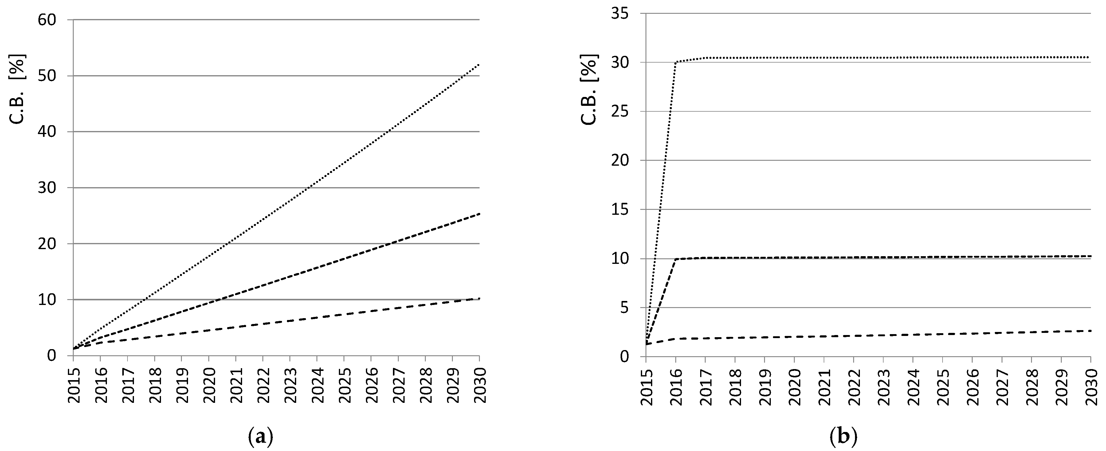
On the other hand, if we use a constant variance value during the whole time horizon, the resulting confidence intervals associated to the forecasted values abruptly increase during the first year and then a phase of a small increase follows (Figure 2b). The behavior of the quality is underlined in Figure 3a,b, which reports the magnitude of the confidence bounds in the six presented scenarios.
The overall entity of the uncertainty at the end of the forecasting horizon is, in any case, quite worrying. The roots of the behavior of “one equation” model are found in Equations (1) and (6). According to the model, the sensitivity of the forecasted value with respect to state and control variables, that is the coefficients reported in Table 5, controls the evolution of the covariance matrix.
The variance behavior of the ln(Cres) follows from Equation (6). It is composed of two terms; the first representing the propagation of the state variance and the second accounting for the injection due to the exogenous inputs. The time history of these components is reported in Table 6 with reference to the constant variance addition, 10% case, see Figure 3b. The squared values of the (1, 1) element are reported.
Since the state variables are the natural log of the original variable, the value can be directly interpreted as a fraction value of Cres confidence interval. In other words, the last column specifies a value of the 95% confidence interval equal to about 10% of the Cres value.
The fact that the final magnitude of the Cres confidence is similar to the confidence assumed for the explanatory variables is casual and results from the particular values of the elasticities in this specific case.
After a short transient phase, it appears that the confidence of Cres, after a reduction due to model propagation (Table 5 column B), reaches a quasi-steady state (column D) with the addition of variance that accounts for the control uncertainty (column C). This fact appears a somewhat favorable element but it must be noted that this result is obtained only in case of constant uncertainty affecting the explanatory variables. It seems more realistic that the constant rate increase better represents the difficulty to make prediction when the involved times are more and more remote.
Finally, it is noted that if the model utilized to describe the proposed scenario is exact (typically in simulated tests, where the model underlying the simulated data is the same used by the forecasting algorithm), no problem arises during the model identification process and correct results can be found also in the presence of large observation errors. If, as it seems to happen in this study, our description of the phenomenon contains some known or unknown approximations and incorrectness (e.g., possible oversimplification of the “one equation” model), the identification of unknown parameters may become unreliable, especially if results are extrapolated to predict future performance. In fact, the inverse solution algorithm, whose primary target is to minimize the residuals of the term “ln(Cres)”, might compensate the model incorrectness with a wrong choice of parameters and a good fitting on observed data does not always guarantee a good forecasting. Various techniques can be implemented in these conditions, for example the use of proper process noise covariance matrix (separate from the control noise covariance) to account for model mismatches. In any case, obviously, the more the algorithm model differs from the real one, the more biased the forecasting will be [35].
Anyway, it should be always considered the optimal trade-off between the complexity of the model and the accuracy of the results, because the risk is to complicate more than necessary energy consumption models by introducing, for instance, new parameters and links towards external variables, which require a number of inputs difficult to find in the usual available statistics [36].
5. Conclusions
Forecasting results concerning natural gas consumption coming from a standard regression technique has been validated by using a Kalman filter. Then, the model behavior has been studied by means of standard covariance propagation analysis to assess the quality of the obtained estimates.
From the results, it reasonably appears that the commonly used “one equation” approach, at least in the presented case, causes the forecasted variable to be very sensitive to errors in the explanatory variables. While this is not a serious issue during the fitting phase of historical data, problems arise when the selected formula is used to predict future scenarios.
As a consequence, a great care must be taken when the forecast horizon extends over many years and it is necessary to analyze and check the explanatory variables in order to investigate their accuracy, which represents a fundamental aspect of the whole forecasting process.
Another approach might be represented by the implementation of more sophisticated models able to include the multi-level interconnections among the variables. To mimic these mutual correlations, it would be better to improve the basic model to include more and more explanatory variables (but avoiding over-specification, i.e., the inclusion of redundant predictor variables [37]), along with their models, in order to better describe the nature of the real word dynamics. To tackle such an integrated approach, it may be better to model primary energy consumption as a set of equations in which the interactions with the “surrounding” are pushed further and further away to provide a kind of smoothing of the errors coming from the exogenous input. The correctness of this approach will be confirmed, or not, by an analysis of the variance evolution.
Acknowledgments
The authors want to acknowledge Luca A. Tagliafico for the useful discussion concerning the subject of the present paper. The present work was supported by Italian Ministry of University and Research MIUR (PRIN 2015, grant n. 2015M8S2PA).
Author Contributions
Federico Scarpa and Vincenzo Bianco conceived and designed the case study and the analysis; Vincenzo Bianco analyzed the data and tuned the model; Federico Scarpa analyzed the data in the forecasting phase; Federico Scarpa and Vincenzo Bianco wrote the paper.
Conflicts of Interest
The authors declare no conflict of interest.
References
- Olanrewaju, O.A.; Jimoh, A.A. Review of energy models to the development of an efficient industrial energy model. Renew. Sustain. Energy Rev. 2014, 30, 661–671. [Google Scholar] [CrossRef]
- Zarnikau, J. Functional forms in energy demand modeling. Energy Econ. 2003, 25, 603–613. [Google Scholar] [CrossRef]
- Bianco, V.; Scarpa, F.; Tagliafico, L.A. Long term outlook of primary energy consumption of the Italian thermoelectric sector: Impact of fuel and carbon prices. Energy 2015, 87, 153–164. [Google Scholar] [CrossRef]
- Bianco, V.; Manca, O.; Nardini, S. Linear regression models to forecast electricity consumption in Italy. Energy Sources Part B Econ. Plan. Policy 2013, 8, 86–93. [Google Scholar] [CrossRef]
- Irsag, B.; Puksec, T.; Duic, N. Long term energy demand projection and potential for energy savings of Croatian tourism-catering trade sector. Energy 2012, 48, 398–405. [Google Scholar] [CrossRef]
- Suganthi, L.; Samuel, A.A. Energy models for demand forecasting—A review. Renew. Sustain. Energy Rev. 2012, 16, 1223–1240. [Google Scholar] [CrossRef]
- Huntington, H.G. Industrial natural gas consumption in the United States: An empirical model for evaluating future trends. Energy Econ. 2007, 29, 743–759. [Google Scholar] [CrossRef]
- Sailor, D.J.; Muñoz, J.R. Sensitivity of electricity and natural gas consumption to climate in the U.S.A.—Methodology and results for eight states. Energy 1997, 22, 987–998. [Google Scholar] [CrossRef]
- Potočnik, P.; Soldo, B.; Šimunović, G.; Šarić, T.; Jeromen, A.; Govekar, E. Comparison of static and adaptive models for short-term residential natural gas forecasting in Croatia. Appl. Energy 2014, 129, 94–103. [Google Scholar] [CrossRef]
- Iranmanesh, H.; Abdollahzade, M.; Miranian, A. Mid-term energy demand forecasting by hybrid neuro-fuzzy models. Energies 2012, 5, 1–21. [Google Scholar] [CrossRef]
- Bianco, V.; Scarpa, F.; Tagliafico, L.A. Scenario analysis of nonresidential natural gas consumption in Italy. Appl. Energy 2014, 113, 392–403. [Google Scholar] [CrossRef]
- Soldo, B.; Potočnik, P.; Šimunović, G.; Šarić, T.; Govekar, E. Improving the residential natural gas consumption forecasting models by using solar radiation. Energy Build. 2014, 69, 498–506. [Google Scholar] [CrossRef]
- Lü, X.; Lu, T.; Kibert, C.J.; Viljanen, M. Modeling and forecasting energy consumption for heterogeneous buildings using a physical-statistical approach. Appl. Energy 2015, 144, 261–275. [Google Scholar] [CrossRef]
- Shaikh, F.; Ji, Q.; Shaikh, P.H.; Mirjat, N.H.; Uqaili, M.A. Forecasting China’s natural gas demand based on optimised nonlinear grey models. Energy 2017, 140, 941–951. [Google Scholar] [CrossRef]
- Shaikh, F.; Ji, Q. Forecasting natural gas demand in China: Logistic modelling analysis. Electr. Power Energy Syst. 2016, 77, 25–32. [Google Scholar] [CrossRef]
- Szoplik, J. Forecasting of natural gas consumption with artificial neural networks. Energy 2015, 85, 208–220. [Google Scholar] [CrossRef]
- Soldo, B. Forecasting natural gas consumption. Appl. Energy 2012, 92, 26–37. [Google Scholar] [CrossRef]
- Amarawickrama, H.A.; Hunt, L.C. Electricity demand for Sri Lanka: A time series analysis. Energy 2008, 33, 724–739. [Google Scholar] [CrossRef] [Green Version]
- Khan, M.A. Modelling and forecasting the demand for natural gas in Pakistan. Renew. Sustain. Energy Rev. 2015, 49, 1145–1159. [Google Scholar] [CrossRef]
- Akpinar, M.; Yumusak, N. Year ahead demand forecast of city natural gas using seasonal time series methods. Energies 2016, 9, 727. [Google Scholar] [CrossRef]
- Bianco, V.; Scarpa, F.; Tagliafico, L.A. Analysis and future outlook of natural gas consumption in the Italian residential sector. Energy Convers. Manag. 2014, 87, 754–764. [Google Scholar] [CrossRef]
- Inglesi-Lotz, R. The evolution of price elasticity of electricity demand in South Africa: A Kalman filter application. Energy Policy 2011, 39, 3690–3696. [Google Scholar] [CrossRef]
- Nguyen, H.T.; Nabney, I.T. Short-term electricity demand and gas price forecasts using wavelet transforms and adaptive models. Energy 2010, 35, 3674–3685. [Google Scholar] [CrossRef]
- Song, H.; Liu, X.; Romilly, P. A time varying parameter approach to the Chinese aggregate consumption function. Econ. Plan. 1996, 29, 185–203. [Google Scholar] [CrossRef]
- Pappas, S.S.; Ekonomou, L.; Karamousantas, D.C.; Chatzarakis, G.E.; Katsikas, S.K.; Liatsis, P. Electricity demand loads modeling using Auto Regressive Moving Average (ARMA) models. Energy 2008, 33, 1353–1360. [Google Scholar] [CrossRef]
- Erdogdu, E. Electricity demand analysis using cointegration and ARIMA modelling: A case study of Turkey. Energy Policy 2007, 35, 1129–1146. [Google Scholar] [CrossRef] [Green Version]
- Haas, R.; Schipper, L. Residential energy demand in OECD-countries and the role of irreversible efficiency improvements. Energy Econ. 1998, 20, 421–442. [Google Scholar] [CrossRef]
- Karanfil, F.; Ozkaya, A. Estimation of real GDP and unrecorded economy in Turkey based on environmental data. Energy Policy 2007, 35, 4902–4908. [Google Scholar] [CrossRef]
- Engle, R.F.; Watson, M.W. The Kalman filter: Applications to forecasting and rational expectations models. In Advances in Econometrics; Bewley, T.F., Ed.; Fifth World Congress; Cambridge University Press: Cambridge, UK, 1987; Volume 1, pp. 245–284. ISBN 9781139052061. [Google Scholar]
- Arisoy, I.; Ozturk, I. Estimating industrial and residential electricity demand in Turkey: A time varying parameter approach. Energy 2014, 66, 959–964. [Google Scholar] [CrossRef]
- Candy, J.V. Signal Processing: The Model Based Approach; McGraw-Hill: New York, NY, USA, 2008; ISBN 0070665559. [Google Scholar]
- Kraus, M. Energy forecasting. The epistemological context. Futures 1987, 19, 254–275. [Google Scholar] [CrossRef]
- ISTAT. Italian Institute of Statistics. 2014. Available online: http://dati.istat.it/ (accessed on 15 September 2017).
- OECD. Economic Outlook. 2012, 91, Table 4.1. Available online: http://www.oecd-ilibrary.org/economics/oecd-economic-outlook-volume-2012-issue-1_eco_outlook-v2012-1-en (accessed on 15 September 2017).
- Candy, J.V. Model-Based Signal Processing; IEEE Press, Wiley-Interscience: Hoboken, NJ, USA, 2006; ISBN 9780471236320. [Google Scholar]
- Holton, J.; Keating, B. Business Forecasting; McGraw Hill: New York, NY, USA, 2009; ISBN 0073373648. [Google Scholar]
- Guajarati, D. Basic Econometrics; McGraw Hill: New York, NY, USA, 2004; ISBN 0073375772. [Google Scholar]
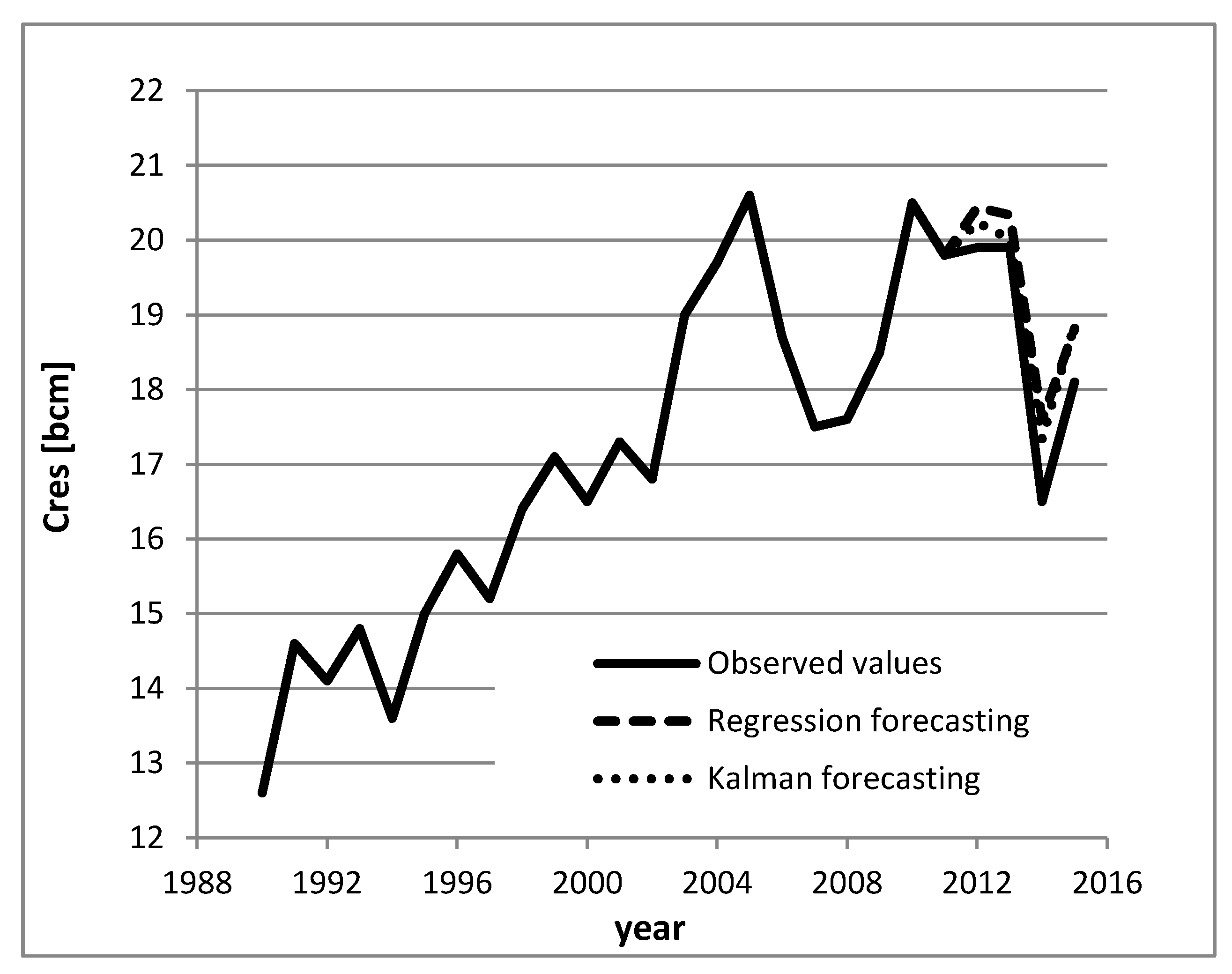
Figure 1.
Validation phase. Cres values. Observer data in the period 1990–2011 (continuous line) and forecasted values in the years 2012–2015; Regression algorithm (dashed line) and Kalman algorithm (dotted line).
Figure 1.
Validation phase. Cres values. Observer data in the period 1990–2011 (continuous line) and forecasted values in the years 2012–2015; Regression algorithm (dashed line) and Kalman algorithm (dotted line).

Figure 2.
Forecasted values of natural gas consumption, Cres, and associated 95% confidence bounds. (a) Linear increase of the std. dev. associated to the exogenous variables, three different rates starting from 1.5% up to 10%, 25% and 50% at the end of the time horizon; (b) Constant std. dev. during the whole time horizon, three different levels; 1.5%, 10% and 30%.
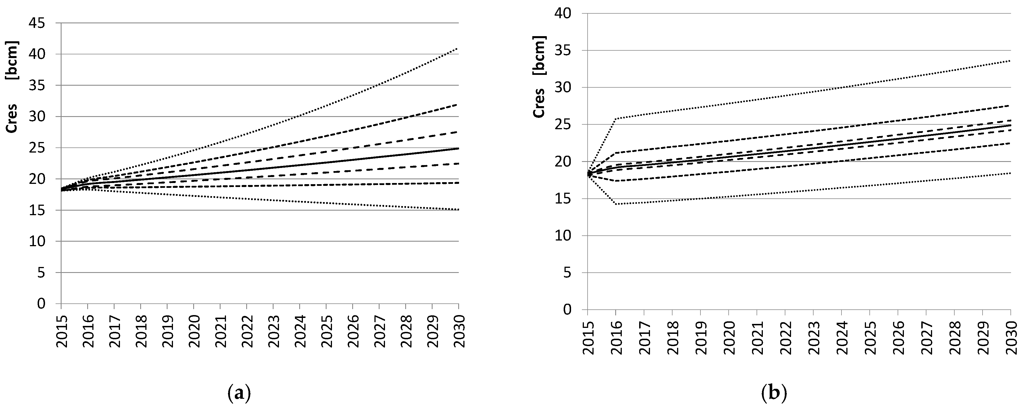
Figure 3.
Average 95% confidence intervals as a percentage of the Cres value. (a) Linear increase of the std. dev. associated to the exogenous variables, three different rates; (b) Constant std. dev. during the whole time horizon, three different levels. See Figure 2.
Figure 3.
Average 95% confidence intervals as a percentage of the Cres value. (a) Linear increase of the std. dev. associated to the exogenous variables, three different rates; (b) Constant std. dev. during the whole time horizon, three different levels. See Figure 2.

Table 1.
Reference data (observed values) for Cres, gross domestic product (GDP), Pres and heating degree days (HDD).
Table 1.
Reference data (observed values) for Cres, gross domestic product (GDP), Pres and heating degree days (HDD).
| Year | Cres [bcm] | GDP [€] | Pres [€ GJ−1] | HDD [°C Days] |
|---|---|---|---|---|
| 1990 | 12.6 | 12,365.3 | 13.8 | 1884 |
| 1991 | 14.6 | 13,492.3 | 15.8 | 2234 |
| 1992 | 14.1 | 14,185.3 | 16.2 | 1886 |
| 1993 | 14.8 | 14,600.2 | 14.0 | 1973 |
| 1994 | 13.6 | 15,440.8 | 14.4 | 1797 |
| 1995 | 15.0 | 16,665.5 | 13.5 | 1929 |
| 1996 | 15.8 | 17,653.4 | 14.5 | 1938 |
| 1997 | 15.2 | 18,434.9 | 16.2 | 1807 |
| 1998 | 16.4 | 19,178.1 | 15.8 | 1902 |
| 1999 | 17.1 | 19,802.6 | 15.2 | 1883 |
| 2000 | 16.5 | 20,917.0 | 16.5 | 1695 |
| 2001 | 17.3 | 21,914.9 | 18.0 | 1767 |
| 2002 | 16.8 | 22,660.7 | 17.0 | 1711 |
| 2003 | 19.0 | 23,181.3 | 17.0 | 1913 |
| 2004 | 19.7 | 23,919.6 | 15.0 | 1883 |
| 2005 | 20.6 | 24,390.9 | 15.6 | 2051 |
| 2006 | 18.7 | 25,200.9 | 17.1 | 1824 |
| 2007 | 17.5 | 26,040.8 | 17.9 | 1715 |
| 2008 | 17.6 | 26,204.1 | 18.8 | 1776 |
| 2009 | 18.5 | 25,465.0 | 18.2 | 1829 |
| 2010 | 20.5 | 26,224.3 | 19.6 | 1992 |
| 2011 | 19.8 | 26,602.0 | 21.9 | 1861 |
| 2012 | 19.9 | 26,254.7 | 24.3 | 1968 |
| 2013 | 19.9 | 25,589.1 | 24.8 | 1933 |
| 2014 | 16.5 | 25,702.7 | 24.7 | 1603 |
| 2015 | 18.1 | 26,003.1 | 23.6 | 1810 |
Table 2.
Assumed initial condition and measurement quality.
| Parameter | Initial Value | Quality (1.96σ) |
|---|---|---|
| β0, …, β5 | 0.5 | 6 (∞) |
| Control noise | - | Varied (see analysis) |
| Observation noise | - | 1.5% |
Table 3.
Validation phase. Cres values. Model identification phase: 1990–2011. A 95% confidence interval equal to ±1.5% for all the explanatory variables has been assumed. Forecasting interval: 2012–2015. Standard regression compared to Kalman filter forecasting. The percentage errors in respect to the observed values are reported too.
| Year | ObservedValues (bcm) | Regression Forecasting (bcm) | Kalman Forecasting (bcm) | Percentage Difference Regr vs. Kalman | Cres Estimated 95% Confidence (bcm) |
|---|---|---|---|---|---|
| 2012 | 19.91 | 20.44 (+2.7%) | 20.24 (+1.7%) | −1.0% | ±2.5% |
| 2013 | 19.86 | 20.34 (+2.4%) | 20.02 (+0.8%) | −1.5% | ±3.1% |
| 2014 | 16.55 | 17.60 (+6.4%) | 17.34 (+4.8%) | −2.0% | ±3.3% |
| 2015 | 18.10 | 18.82 (+4.0%) | 18.88 (+4.3%) | +0.3% | ±3.1% |
Table 4.
Forecasting results. Cres values. Standard regression compared to Kalman filter forecasting. The percentage differences are reported in the last column.
Table 4.
Forecasting results. Cres values. Standard regression compared to Kalman filter forecasting. The percentage differences are reported in the last column.
| Year | Regression Forecasting (bcm) | Kalman Forecasting (bcm) | Percentage Difference Regr vs. Kalman |
|---|---|---|---|
| 2027 | 23.48 | 23.50 | +0.080% |
| 2028 | 23.93 | 23.95 | +0.071% |
| 2029 | 24.40 | 24.41 | +0.064% |
| 2030 | 24.87 | 24.88 | +0.055% |
Table 5.
Model parameters found from data of Table 1.
Table 5.
Model parameters found from data of Table 1.
| Algorithm | β0 | β1 | β2 | β3 | β4 | β5 |
|---|---|---|---|---|---|---|
| Standard regression | −5.42 | 0.834 | −0.174 | 0.479 | 0.256 | 0.103 |
| Kalman filter | −5.28 | 0.829 | −0.162 | 0.529 | 0.163 | 0.092 |
Table 6.
Steady state behavior of ln(Cres) variance and its components, as from Equation (6).
| Year | A | B | C | D |
|---|---|---|---|---|
| 2024 | 0.10119 | 2.32 × 10⁻² | 9.86 × 10⁻² | 0.10132 |
| 2025 | 0.10132 | 2.38 × 10⁻² | “ | 0.10146 |
| 2026 | 0.10146 | 2.44 × 10⁻² | “ | 0.10160 |
| 2027 | 0.10160 | 2.50 × 10⁻² | “ | 0.10175 |
| 2028 | 0.10175 | 2.57 × 10⁻² | “ | 0.10191 |
| 2029 | 0.10191 | 2.64 × 10⁻² | “ | 0.10210 |
| 2030 | 0.10210 | 2.70 × 10⁻² | “ | 0.10226 |
© 2017 by the authors. Licensee MDPI, Basel, Switzerland. This article is an open access article distributed under the terms and conditions of the Creative Commons Attribution (CC BY) license (http://creativecommons.org/licenses/by/4.0/).
Share and Cite
MDPI and ACS Style
Scarpa, F.; Bianco, V. Assessing the Quality of Natural Gas Consumption Forecasting: An Application to the Italian Residential Sector. Energies 2017, 10, 1879. https://doi.org/10.3390/en10111879
AMA Style
Scarpa F, Bianco V. Assessing the Quality of Natural Gas Consumption Forecasting: An Application to the Italian Residential Sector. Energies. 2017; 10(11):1879. https://doi.org/10.3390/en10111879
Chicago/Turabian StyleScarpa, Federico, and Vincenzo Bianco. 2017. "Assessing the Quality of Natural Gas Consumption Forecasting: An Application to the Italian Residential Sector" Energies 10, no. 11: 1879. https://doi.org/10.3390/en10111879
Note that from the first issue of 2016, this journal uses article numbers instead of page numbers. See further details here.