Anti-Freezing Mechanism Analysis of a Finned Flat Tube in an Air-Cooled Condenser


Key Laboratory of Condition Monitoring and Control for Power Plant Equipment, North China Electric Power University, Ministry of Education, Beijing 102206, China
*
Author to whom correspondence should be addressed.
Energies 2017, 10(11), 1872; https://doi.org/10.3390/en10111872
Submission received: 21 September 2017
/
Revised: 8 November 2017
/
Accepted: 9 November 2017
/
Published: 15 November 2017
Abstract
:In cold winter weather, the air-cooled condensers (ACCs) face serious freezing risks, especially with part load of the power generating unit. Therefore, it is of benefit to investigate the heat transfer process between the turbine exhaust steam and cooling air, by which the freezing mechanism of the finned tube bundles can be revealed. In this work, the flow and heat transfer models of the cooling air coupling with the circulating water, are developed and numerically simulated for the anti-freezing analysis on basis of the finned tube bundles of the condenser cell. The local air-side heat transfer coefficient, condensate film development, and non-condensable gas development are obtained and analyzed in detail. The results show that, the most freezing risk happens at the fin base due to the highest air-side cooling capacity, besides the windward velocity, ambient temperature and turbine back pressure all determine the freezing risk with the constant inlet flow rate of the non-condensable gas. Furthermore, increasing fin thickness and decreasing fan rotating speed are the most effective anti-freezing measures. Additionally, increasing turbine back pressure can also be adopted to avoid ACC freezing, however the adjustment of outlet steam-air flow is not recommended.
1. Introduction
Air cooled condensers (ACCs) have been increasingly developed in large scale thermal power plants around the world, owing to their substantial water conservation [1]. Generally, an ACC consists of dozens of condenser cells in a rectangular array, and each condenser cell is composed by “Λ” frame finned tube bundles with an axial flow fan below so that ambient air can be driven to pass through the heat exchangers to remove the heat rejection from exhaust steam. However, in cold winter, the cooling air can easily take away the entire heat load of the exhaust steam, which result in a freezing risk of the finned tube bundles. In such a case, it is necessary to study the heat transfer mechanism between the cold air and exhaust steam, which may be beneficial to the safe and energy efficient operation of ACC in power plants.
In past decades, the air-side thermo-flow performances of finned tube bundles have been thoroughly investigated by means of wind tunnel experiments [2,3], as well as numerical simulations [4,5]. Nebuloni and Thome proposed a theoretical and numerical model to predict film condensation and flow boiling heat transfer in mini and micro-channels of different internal shapes [6,7,8,9]. However, most attention was paid to the thermal resistance of cooling air, and few studies have been carried out on the anti-freezing issues of ACCs. It’s worth noting that the cooling air in cold winter has a huge heat capacity when it flows through the condenser cell, and can carry off the maximum heat load of the turbine exhaust steam. Furthermore, for the counter-flow heat exchangers of ACCs, the freezing risk occurs more intentionally because that as the end of the in tube condensation process, the air leaking into low pressure tube side is rich. As also noticed, although the finned flat tube has more advantages in preventing ACC freezing [10], freezing risks still happen in most direct dry cooling systems in northern China when the power load is lowered. Conclusively, it is critical to investigate the mechanisms of steam condensation as well as the thermo-flow characteristics of cold air for the heat exchanger bundles of ACCs.
With regard to the freezing mechanism, several studies have focused on the multi-row tube bundles [11,12]. Besides, some operating measures in practical engineering such as the control logic and adjustment were also proposed for the axial flow fans in ACC power plants [13,14]. On the other hand, Wang [15] raised the total mass flow rate of circulating water to avoid the freezing risk in a natural draft dry cooling system, and switched off the sectors which are most likely affected further [16]. Chen [17] concentrated on the airside by adapting the opening degree of the louvers, but unfortunately, the freezing mechanisms as well as anti-freezing measures for single row finned flat tubes which are usually adopted for ACC, have hardly been mentioned. In this research, the numerical and mathematical models of finned tube bundles for ACCs are established to characterize the local air-side heat transfer coefficient, development of condensate film, and non-condensable gas impacts, which may disclose the freezing mechanism of ACCs. What’s more, the dominant parameters as the steam inlet flow rate, non-condensable gas density, windward velocity, ambient temperature, as well as turbine back pressure are investigated for their effects on the anti-freezing of air-cooled condenser. This research may contribute to the safe and energetic operation of ACCs in power plants.
2. Modeling and Methods
2.1. Physical Model
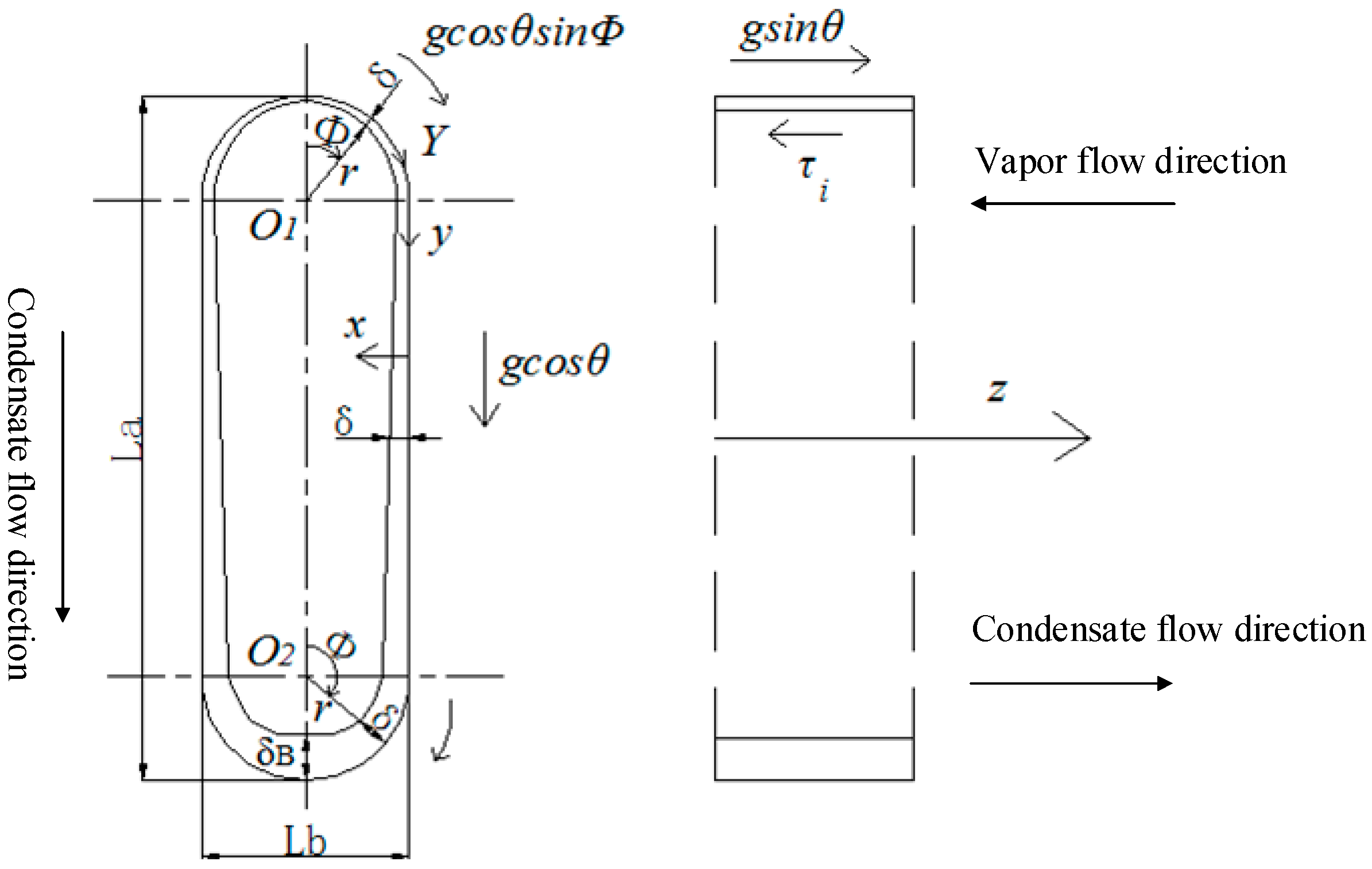
The three-dimensional heat exchanger bundle of the condenser cell in a typical ACC is shown in Figure 1a. The exhaust steam flows into a flat tube bundle from the bottom, while the cooling air flows through the wavy fins along the long axis of the tube. Generally, the finned tube bundle is settled with a slant angle of 60° to horizontal direction. The detailed geometric parameters are shown in Figure 1b.
2.2. Numerical Model
In our study, ANSYS FLUENT is selected as the CFD tool to explore the heat transfer process. The numerical domain is shown in Figure 2a, which is separated into three sections so that the air flow and heat transfer characteristics, development of condensate film around the inside the tube wall, as well as the mass transfer between steam and non-condensable air mixtures on vapor-liquid interface inside the tube, can be obtained. For the computational domain, the grid independence is carried out with the final grid number as 501,032.
As further pointed out, the thermo-flow performances of cooling air provide the local heat transfer coefficients, so the convective boundary is calculated to achieve the steam condensation with the effects of the non-condensable gas also considered. As shown in Figure 2 for the side view of finned flat tube, it is divided into four typical sections, namely the air flow inlet arc as region 1, the air flow outlet arc as region 2, the flat tube wall with fins as region 3, and the flat tube wall without fins as region 4. For each section, the air-side convective heat transfer coefficient can be obtained by the numerical model except for region 3, which gives as follows:
Q is heat rate, Δtm is logarithmic average temperature difference, Ar is the surface area of tube base wall, and ηf is the fin efficiency. The air-side convective heat transfer coefficient will provide a boundary for the further analysis.
For the air flow and heat transfer characteristics of the finned flat tube, the governing equations are developed. Since the heat exchanger used in this paper is the same as the [18], moreover, the simulation carried before with k-omega model is based on a rectangular finned elliptical tubes, the kω-SST model is adopted for closing the governing equations due to the good prediction for the turbulence flow of viscous fluid [18]. Such an improvement is verified further in Menter’s work [19]. As shown in Figure 2, the computational domain is extended for the sufficient upstream and downstream air flows. The base wall temperature of flat tube is set as a constant. The top and bottom faces are appointed as the periodic boundaries, while the fin wall as coupling conduction boundary.
The upstream and downstream surfaces are respectively set as velocity inlet and pressure outlet boundaries. The detailed meshes for the dry cooling tower and heat exchanger are shown in Figure 2b. For the central part, hexahedral structured grids are taken thanks to their regular and simple shape. For other sections, the tetrahedral unstructured grids are adopted due to the complicated geometric structure. The total number of cells in the inlet section and outlet section are 23,628 and 164,784 with the maximum skewness of 0.489806 and 0.396817 particularly, while the cells number of the tube section are 91,200 with a maximum skewness of 1.31328 × 10⁻¹⁰. Furthermore, the pressure-based solver is used to discretize the governing equations, with the SIMPLE algorithm of pressure-velocity coupling employed. Under a steady running condition, the air-side flow and heat transfer governing equations take the following form:
The second-order upwind differencing scheme is applied to the discretization of the governing equations for the momentum, energy, turbulent kinetic energy and its dissipation rate. A divergence-free criterion of 10−4 based on the scaled residual is prescribed for the computations.
2.3. Condensate Film Development Inside Finned Flat Tube
With the aforementioned heat transfer coefficients, the boundaries can be set for the flow condensation model. For the steam flow condensation in tube, as well as the two-phase flow regime map, many investigations have been carried out, scholars have proposed many theoretical models about the steam flow condensation in tube, including VOF [20], Level set [21] and the interface tracking method [22,23,24,25,26,27,28]. Both VOF and the Level set model are based on the number of grids, so as a result, one can hardly obtain an accurate result when the film is thin enough. In the view of interface tracking method, Wang et al. [22,23,24] utilized the integral method and obtained the condensate film development equation to predict film condensation in micro-channels. Fiedler et al. [25,26,27,28] presented a study of stratified flow pattern for laminar reflux condensation of a pure saturated vapor in an inclined small diameter circular tube. In this research, a stratified flow pattern is assumed by the typical gravity driven condensation process. The interface tracking method is used to solve the hyperbolic equation, therefore the flow condensation model can be established. It is worth noting that, the flat tube wall is divided into four regions as aforementioned above, so the effects of the outside cooling air flow are specifically taken into consideration.
When the wet steam flows into the flat tube, the condensation begins and the condense film is formed on the inner wall of tube due to the cooling effects by air. Figure 3 shows the mechanisms of the flow and heat transfer process between the exhaust steam and cooling air in three dimensions. Y is the half curve length of the upper arc. x equals the distance from tube wall to the vapor-liquid interface, besides the condensate film thickness is measured in x direction. z is the axial direction, describing the axial position. r is the radial polar coordinate with origins as O1 and O2, while φ is the polar angle. In straight wall section, y represents the straight wall height.
Based on the assumption of the stratified flow regime, the condensate flow along the flat tube wall includes two directions, namely the steam main flow direction and the long axial direction of the flat tube which is caused by gravitational force gcosθ. Furthermore, the vapor shear force tends to pull the condensate in the main flow direction. Additionally, the weak surface tension is considered in the arc region, which may pull the condensate film in the peripheral direction.
In order to obtain the inside flow performances of the finned tube, the momentum, energy and diffusion equations for steam-air mixture and the momentum and energy equations for condensate film must be solved simultaneously. What’s more, the energy as well as mass conversation of the condensing constituents is taken consideration, so that the interfacial mass flux of non-condensable gas can be kept as zero.
2.4. Mathematical Model of Condensation
The experiment has been carried out in our previous work [29]. A water cooled visualization condensation test system is designed and built for an indirect study on the flow regime of condensation process in a condenser. Base on the observed stratified flow regime, a theoretical model is built for condensation flow and heat transfer process including condensate water bath development on the arc wall and condensate film development on the other wall. Especially, for condensate film on the wall, a hyperbolic equation is proposed. Considering the convection and conservation characteristic in the equation, a solution algorithm for steady conservation equation is produced by combination of the conjugate gradient method, the Newton method and simulated annealing method, which can avoid the complex of traditional non-steady method. The visualization results indicate that the flow regime of condensation process is stratified flow regime and the corresponding theoretical calculation results indicate that the condensate film thickness on the wall is far less than condensate bath height, which is in the 1 mm order of magnitude, and leads to high condensation heat transfer coefficient. The results supply grounds for judging the onset position of freezing in flat tube under air cooling condition in power plant in winter.
The mass flow rate of steamside varies specifically from 58, 47.5, 38.5, 29 and 23 kg·h−1. The mass flow rate of waterside is adjusted until the steam is condensated. And the results show the mass flow rate varies from 650, 500, 370, 310 and 250, specifically. According to the experimental observation, the condensation happens in the typical regions as the top arc, the side wall, and the bottom condensate pool. The mathematical models are specifically described as follows.
2.4.1. Top Arc Region
The steady-state flow is assumed with considering the various force balances as the shear stress, gravity, and pressure gradient induced by surface tension. The momentum equation in the peripheral direction is expressed by:
where uφ is the velocity component in peripheral direction, and pt is the pressure difference due to the effect of surface tension, which gives:
where σ is the surface tension coefficient and rc is the radius of the condensation surface given by:
The momentum equation in the axial direction for condense pool on the semicircle wall follows:
The energy equation takes:
The boundaries for the Equations (2), (5) and (6) are listed as follows:
For r = R:
For r = ri = R − δi:
where the interface shear stress is given by:
where the first term results from interface shear stress without interface mass transfer, and the second term corresponds to the momentum transfer induced by interface mass transfer. The steam velocity wv can be obtained from local steam flow and position of phase interface. The liquid interface velocity wl,i results from Equation (5). The friction factor cf results from reference [30], given by integrating Equations (2), (5) and (6) subject to boundary conditions (7)–(11) across the film yields:
Further, the condense flow rate in the peripheral direction and the axial direction of grid is:
where:
For thin condensate film, the pressure in two sides of interface is consistent which abides by boundary theory for the consistent pressure. The pressure of steam main flow can be computed by the Equation (22):
where Ag is the area of steam flow section, and the Si the area of perimeter of the two-phase interface in section.
2.4.2. Straight Wall Region
For the steady-state flow, the momentum equation in the peripheral direction for condense film on the straight wall gives:
where u is the velocity component in peripheral direction, and pt is the pressure difference due to the effect of surface tension, given by Equation (8). rc is the radius of the condensation surface given by:
The momentum equation in the axial direction for condense film on the straight wall follows:
The energy equation of condensate film is:
The boundaries for the Equations (23), (25) and (26) are set:
Integrating Equations (23), (25) and (26) subject to boundary conditions Equations (27)–(31) across the film yields:
Further, the condense flow rate in the peripheral direction and the axial direction of grid is:
2.4.3. Development of Condensation
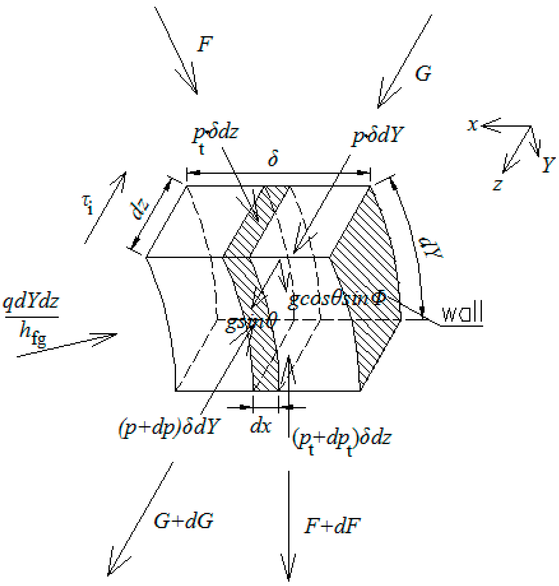
Figure 4 shows the control volume of condensate film on inner wall of flat tube. In the x direction of the fundamental cell, one face is the condensation wall, while the other is the two-phase interface. For the two faces, the condensate from the condensation heat transfer is equivalent to the quality source, and the flow through the two faces is equivalent to zero. F is defined as the control volume condensate flow or the grid peripheral flow in y direction. G is defined as the grid axial flow in z direction.
represents the control volume flux in lower reaches of y axis, and represents increment of control volume flow in circumferential direction. In the same way, represents increment of control volume flow in axial direction. The increment of mass flow of control volume derives from condensation during heat transfer process in heat transfer surface. Q is defined as heat exchange amount of control volume, hfg is latent heat, q is heat flux of control volume, and the control equation can be reported as follows:
where:
Equation (37) can be transformed into Equation (40):
In arc wall region:
In vertical wall region:
Boundary conditions:
Equations (37) or (40), subject to the boundary conditions of Equations (43)–(45) and (52), can be solved numerically by a finite control volume scheme.
2.4.4. Condensate Pool Model
The condensate film is initially formed at the top position of the flat tube and develops along the flow direction. A thin liquid film is formed on the condense wall. However, in the bottom of the tube section, the transition of peripheral velocity from a considerable value to zero is proceeding because of the decreasing gravity component and the increasing normal stress in peripheral direction which hinders the flow in peripheral direction.
It’s worth noting that, the transition process is simplified in this research. Only the axial velocity in the pool is considered which meets the Nusselt assumptions. Furthermore, the straight shape line is applied [25,26,27,28]. During the calculation of pool, the sum of condensate pool flow and condensate wall film flow equals to the sum of the condensate flow before the local z direction distance. So, if the height of the pool is obtained, the condensate pool flow needs to update by the difference between the sum of the condensate flow and the condensate wall film flow above the height of the pool. In such a case, the local condensate pool height is achieved by condensate pool flow iteration and pool height iteration.
2.5. Heat and Mass Transfer Models
As a kind of non-condensable gas, air has a significant impact on condensation. Near the condensation wall, air and steam form a steam-gas mixture layer and the mass transfer process of condensation is deteriorated. The mixture layer increases mass transfer resistance and reduces the partial pressure of steam. A lot of studies have been deeply given on mass transfer resistance, and several typical formulas were proposed. By empirical method, in steam stagnation environment, Uchida et al. [31] obtained a formula relating the heat and mass transfer overall coefficient and non-condensable mass concentration. Rose [32] obtained the vapor-liquid interfacial mass transfer coefficient by approximate theoretically-based equations for a vapor-gas mixture flow based on similar dimensionless heat and mass transfer. Nagae et al. [33,34] proposed two interfacial mass transfer coefficient correlations for laminar mixture flow and turbulent flow based on experiments. RELAP5/MOD3.2 is a software using in nuclear industry, by which the interfacial mass transfer coefficient is obtained by analogy between heat and mass transfer based on the work of Nithianandan et al. [35], Colburn et al. [36]. Peterson [37,38] supplied a simple method to model interfacial mass transfer performance by derived condensation equivalent conduction coefficient, which contributes to experiment measurement greatly. Liao et al. [39] improved the method of condensation equivalent conduction coefficient originally derived on a molar basis by developing that parameter based on a mass basis, which includes effect of variable vapor-gas mixture molecular weights across the diffusion layer on mass diffusion. In this paper, the formula supplied by Nagae [33,34] is used, which provides correlations for laminar mixture flow and turbulent flow based on experiments.
The energy equation at the interface of condensate film and steam-air mixture layer can be described as:
where hδ is pure condensation heat transfer coefficient from condensate film, hg is forced convection heat transfer coefficient, and m″ represents mass transfer rate in condensation process. Tb is average temperature of steam-air mixture and Ti is interface temperature of condensate film. Tb,s is saturation temperature of steam for steam-air mixture, hm is equivalent heat transfer coefficient for mass transfer.
The diffusive mass transfer can be calculated by invoking experiment formula [33,35], which is widely applied in nuclear industry. The convective heat transfer coefficient during condensation can be calculated by classical force convective heat transfer formula. Defined Nug as dimensionless heat transfer coefficient, Num as dimensionless equivalent heat transfer coefficient for mass transfer, and then under laminar flow condition:
where vg is average velocity of steam-air mixture, υg represents viscosity of steam-air mixture and D is equivalent diameter of flat tube:
where λs represents thermal conductivity of steam, ps represents partial pressure of steam and pa is partial pressure of non-condensable gas. The constant parameters in Equation (48) are:
a = 0.0012, b = 1.0
Defined Res as dimensionless steam velocity:
Under turbulent flows:
where:
a = 0.0035, b = 0.8
λg represents thermal conductivity of steam-air mixture and Prg represents Prandtl number.
The convection thermal boundaries are adopted by the aforementioned four kinds of air-side heat transfer coefficients in Section 2.1:
where ha is air-side heat transfer coefficient. Tw is wall temperature. Ta,Y is local air temperature, which can be calculated by grid based ε-NTU method along air flow direction.
3. Result and Discussion
3.1. Typical Case
During the simulation, the condenser wall temperature sets equal to the condensation temperature at any ambient condition. At the same boundary, by means bof the CFD simulations, the mass flow rate of cooling air and inlet air temperature of condensers can be obtained. If the mass flow rate of exhaust steam keeps constant, the condensation temperature ts can be calculated. This calculated ts should be equal to the specified one before simulation, otherwise, a new condensation temperature should be assumed. As can be seen, the numerical simulation is an iterative procedure. The flow chart for the simulation of thermo-flow performances of air-cooled condensers and the net power output of generating units is shown in the following Figure 5.
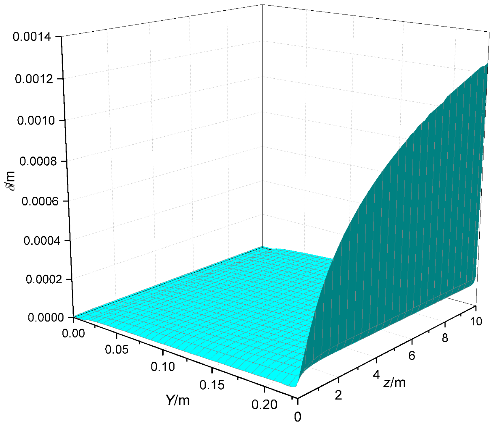
For a typical case with the inlet steam flow of 34.5 kg/h, non-condensable air flow of 0.0139 × 2/10,000 kg/s, back pressure of 10 kPa, windward velocity of 0.5 m/s, the volume flowrate of air is 1 m3/s and environment temperature of −20 °C, the three dimensional distribution of condensate film thickness is obtained, as shown in Figure 6.
As observed, the condensate film distribution in tube inside space is non-uniform. In y direction along periphery of flat tube, most of the condensate flow is distributed in region of Y value less than 0.20 m located at the arc section of flat tube where the condensate pool is formed. The maximum value of the pool height is 1.25 mm, which shows much lower than arc radius of 9.5 mm, while the concentrate film thickness not belonging to liquid pool is less than 0.1 mm.
Figure 7 presents the four representative condensation temperatures for the four characteristic regions of the flat tube. It can be seen that in the y direction of the flat tube, the condensation temperature at the initial position of fin at Y = 0.2149 m is the lowest, even comparing with temperature at Y = 0.2301 m where condensate pool locates. That’s because, in the direction of cooling air flow, the heat flux at the common border between fin and flat tube wall is larger compared to that in region of non-finned flat tube wall due to advanced heat transfer mechanism of fin. Moreover, at the initial position of fin, the air is only heated by non-fin arc region, and the flux at that border can be the largest. Then the condensation temperature at fin initial position dominates the chief characteristic parameter for anti-freezing requirement. The following discussions of freezing risk are all based on development of that parameter in z direction.
It can be concluded that the temperature of condensate water pool should not be focus of freezing issues, due to the little condensate film thermal resistance. For common border between fin and base wall of flat tube, the thermal flux is advanced by fin which can be regarded as the dangerous position.
3.2. Effects of Inlet Steam Flow on Freezing Risk
With the fixed inlet non-condensable gas-air flow of 0.000002778 kg/s for one flat tube, ambient temperature of −20 °C, back pressure of 10 kPa corresponding to saturation temperature of 45.8 °C, windward velocity of 0.5 m/s, the steam-air mixture condensation in finned flat tube is calculated with various inlet steam flows. The effects of steam flow on freezing risk are shown in Figure 8a,b.
It can be seen that, in z direction from 10 m to 0 m, the characteristic condensation temperature decreases, while the gas concentration increases progressively. In Figure 8a, the non-condensation gas concentration far away from steam inlet is very low in the steam flow direction. Meanwhile only near the condensation end region, the concentration begins to increase rapidly and progressively. That’s because, with the regularly decreased steam flow, when the inlet non-condensable gas concentration is very low as 2.2/10,000, the non-condensable gas concentration will not increase sharply until the quantity effect of air becomes remarkable at the end of condensation process. As also observed, the condensation temperature drops with the increased gas concentration in steam flow direction. Figure 8b shows that, at the end section of condensation, when condensation temperature reaches the freezing point, it becomes a constant value after that position which is determined as the starting point of freezing. What’s more, Figure 8b presents the horizontal freezing line, which implies the forward freezing position with the decreased steam flow.
3.3. Effects of Inlet Non-Condensable Gas Flow on Freezing Risk
The impacts of non-condensable gas are quantitatively analyzed on freezing risk of finned tube bundle, as shown in Figure 9. As shown in Figure 9a, the air concentration at the position of freezing keeps constant with increasing of inlet steam flow. From Figure 9b, the outlet flow of the flat tube at an inlet gas flow of 0.0139 × 4/10,000 kg/s is twice that at the onset of freezing. Obviously, the air concentration at the position keeps constant as the non-condensable gas flow increases. Moreover, the freezing risk is determined by intensive parameters such as back pressure, windward velocity, environment air temperature, while the inlet gas flow has nearly no effects on changing the critical freezing gas concentration.
In practical engineering, the non-condensable gas will be extracted from low pressure system by vacuum pump, so the non-condensable gas concentration near the extraction point is highly concentrated. For anti-freezing of finned tube bundle, the outlet non-condensable gas concentration should be lower the critical value under the given boundary conditions. Alternatively, the outlet flow should be higher than the critical value. As noticed, since the outlet flow is limited by vacuum pump performance and can be directly measured in power plant, the critical freezing outlet flow is adopted based on the anti-freezing principle. Figure 9b shows that critical freezing outlet flow increases linearly as the non-condensable gas flow increases. As observed, with the increment of non-condensable gas flow as 0.0139 × 1/10,000 kg/s, the critical freezing outlet flow increases about 0.00002390 kg/s.
3.4. Effects of Ambient Temperature on Freezing Risk
Generally, the finned tube bundles may face freezing risk when the ambient temperature is lower than the critical water freezing point. With the fixed inlet non condensable gas-air flow of 0.000002778 kg/s, back pressure of 10 kPa corresponding to saturation temperature of 45.8 °C, and the windward velocity of 0.5 m/s, the condensation of steam air mixture in finned flat tube at various ambient temperature is calculated, as shown in Figure 10.
As can be seen, with decreasing of environment temperature, critical outlet steam-air mixture flow rises with the decreased air temperature, which implies that the freezing risk will occur if the output from vacuum pump is less than the critical value. Additionally, the critical freezing outlet flow ascents linearly as the ambient temperature drops. With 1 °C decrement of ambient temperature, the critical value increases 0.00003690 kg/s.
3.5. Effects of Windward Velocity on Freezing Risk
The freezing risk aggravates when the wind speed increases. With fixed inlet non-condensable gas flow of 0.000002778 kg/s, back pressure of 10 kPa corresponding to saturation temperature of 45.8 °C, and ambient temperature of −20 °C, the condensation of steam-air mixture in finned flat tube is obtained at various windward velocities.
Figure 11 shows the critical freezing outlet flow versus windward velocity. As can be seen, the critical outlet steam-air mixture flow rises linearly with the increased windward velocity. With 0.1 m/s increase of the windward velocity, the critical freezing outlet flow increases 0.00008445 kg/s. Furthermore, if the windward velocity is set, the residual anti-freezing capacity of finned flat tube can be obtained by comparing the practical outlet flow extracted by vacuum pump and the critical value. In order to meet the anti-freezing requirement, windward velocity must be chosen carefully for ACC in power plants.
3.6. Effects of Back Pressure on Freezing Risk
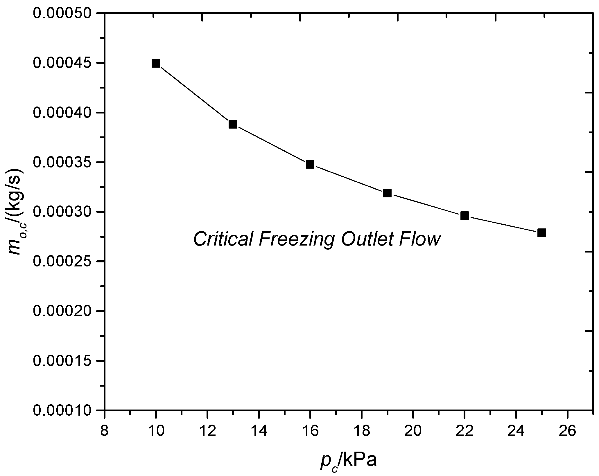
In practical engineering of the power generating unit, the turbine back pressure is usually increased for the anti-freezing of ACC. So the effects of the back pressure on anti-freezing of ACC are specifically studied, with the fixed inlet non-condensable gas flow of 0.000002778 kg/s, ambient temperature of −20 °C, and windward velocity of 0.5 m/s, as shown in Figure 12.
The critical outlet steam-air mixture flow decreases with a decreased gradient as the turbine back pressure increases. Besides, the average value decreases 0.00001428 kg/s as turbine back pressure varies from 10 kPa to 25 kPa. Moreover, for practical operation of ACC in cold winter, the gauge pressures of low pressure devices such as steam turbine and air-cooled condenser, are stable due to the huge pressure difference between the environment pressure and the turbine back pressure. Consequently, the anti-freezing back pressure can be calculated with the fixed non-condensable air flow, ambient temperature and windward velocity.
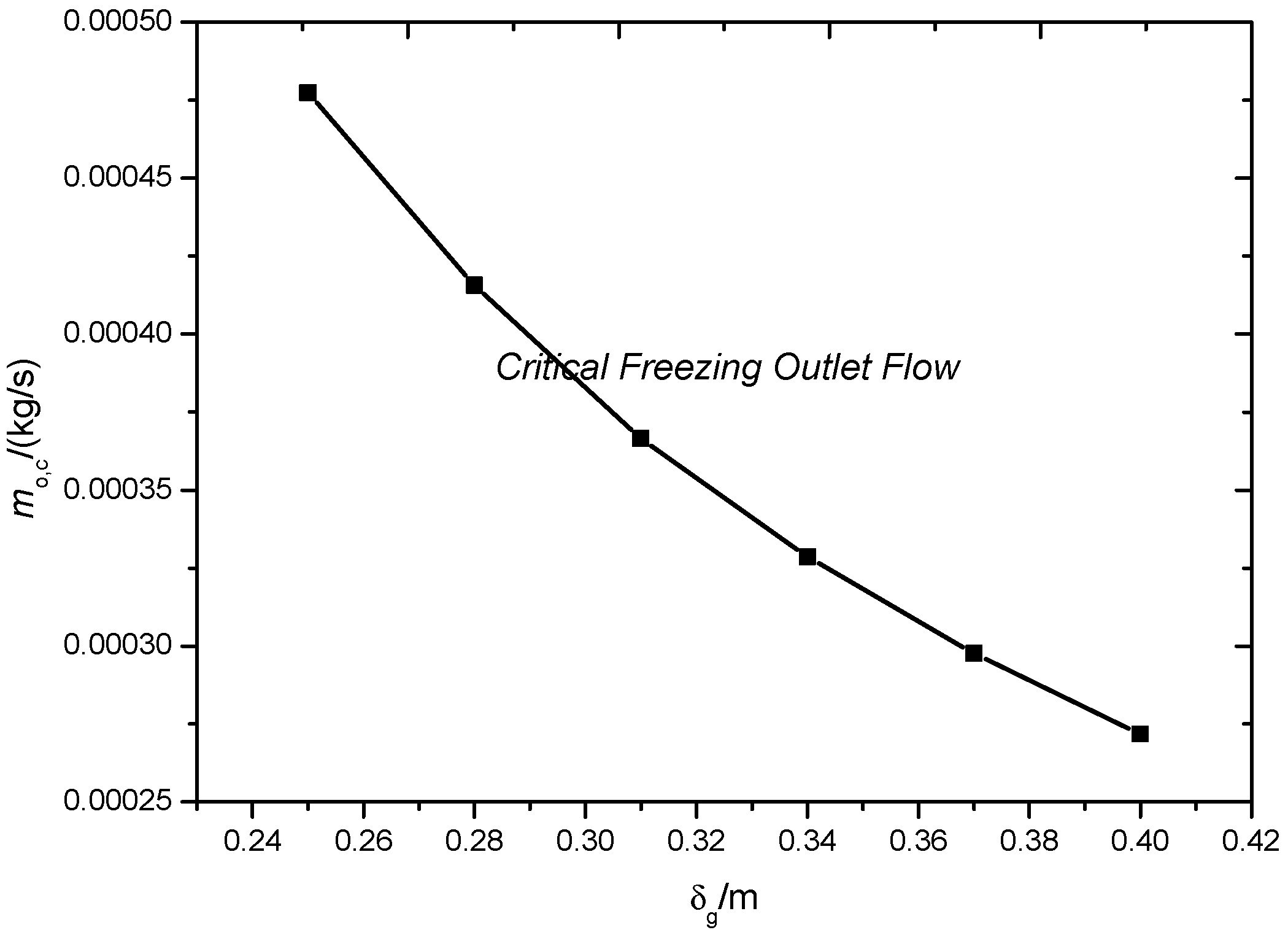
3.7. Effects of Fin Thickness on Freezing Risk
The lowest temperature locates at the interaction between initial fin and base wall of flat tube due to the massive heat flux. Generally, the increased fin thickness can lower down the thermal flux, so the effects of fin thickness on freezing risk are investigated, with the fixed inlet non condensable gas-air flow of 0.000002778 kg/s, ambient temperature of −20 °C, back pressure of 10 kPa and windward velocity of 0.5 m/s. The critical freezing outlet flow versus fin thickness is shown in Figure 13.
Figure 13 shows that the critical outlet steam air mixture flow decreases with the increased fin thickness, implying the weakened freezing risk. As further pointed out, if the fin thickness increases 0.01 mm, the average critical freezing outlet flow decreases 0.00001370 kg/s.
3.8. Adjustment of Critical Freezing Outlet Flow
The impacts from the aforementioned dominant variables on the critical freezing outlet flow are quantitatively summarized in Table 1. As observed, the fin thickness and windward velocity have more obvious effects on the anti-freezing of finned tube bundle, compared with the other three factors.
In practical engineering, some limitations should be taken into account. As a result, increasing the fin thickness stands for the most preferential anti-freezing measure, since the heat flux could be reduced directly, whereas takes little difficulties on manufacture and installation. Additionally, decreasing the fan rotating rate can be adopted in superiority since the windward velocity is lowered down greatly. Furthermore, the adjustment of back pressure could be realized by control logic, which can also achieve the anti-freezing of ACC in power plants. While the ambient temperature belongs to the non-control parameter. As for the non-condensable gas concentration, it is generally determined by gas tightness of air-cooled condenser which cannot be improved timely, thus the anti-freezing of ACC may not be reached flexibly. However, as must be pointed out, if the outlet mixture of condenser can be controlled directly in the future, the anti-freezing can be achieved very well on basis of the anti-freezing principle of cold end system.
4. Conclusions
Freezing risk of ACC is of great concern on frozen days, so its study benefits the safe and energetic operation of ACCs in power generating units. In this research, physical and mathematical models for finned flat tubes are developed, and besides the steam-air condensation and the thermo-flow performances of cooing air are obtained. For air-side modeling, four kinds of local heat transfer coefficients are calculated, which provide the convective thermal boundary conditions for modeling of the steam–air mixture condensation. The adjustment principle of critical freezing outlet flow is proposed, according to the impacts of the dominant factors. The main findings of this research are outlined as follows:
- (1)
- The condensate film on inner flat tube wall has a non-uniform distribution and most of the condensate is formed in the arc region. However, the maximum film thickness at the condensate pool is small, which has little impact on the freezing risk. The lowest temperature occurs at the initial position of the flat fin, resulting from the non-condensable gas collection and big air-side heat capacity.
- (2)
- An adjustment principle of critical freezing outlet flow is proposed. If the outflow of low pressure system is higher than the critical freezing outlet flow, the freezing risk of finned tube bundle can be prevented for ACCs. What’s more, the anti-freezing capacity can be calculated referring to the critical freezing value.
- (3)
- Anti-freezing measures of ACCs are given. In practical engineering, increasing the fin thickness and decreasing the fan rotating speed are proposed as a priority. Besides, increasing the back pressure based on the control logic could also be adopted. However, the adjustment of outlet steam-air flow may not be recommended due to the fixed sealing performance of cold end system.
Acknowledgments
This work was financially supported by State Grid Science and Technology Program (No. GTLN201706-KJXM001 and the national “973 Program” of China (No. 2015CB251505).
Author Contributions
Xiaoze Du provided the main idea of the study; Yonghong Guo, Tongrui Cheng developed the model and analyzed the data; Lijun Yang provided language support and revised the paper.
Conflicts of Interest
The authors declare no conflicts of interest.
Nomenclature
| A | area of section (m2) |
| cf | friction coefficient for single phase |
| D | equivalent diameter of flat tube (m) |
| F | condensate flow of grid in circumferential direction, (kg·s−1) |
| g | acceleration of gravity, (m·s−2) |
| G | condensate flow of grid in axial direction, (kg·s−1) |
| h | heat transfer coefficient ( W·m−2·°C−1) |
| hfg | latent heat, (kJ·kg−1) |
| m | steam flow (kg·s−1) |
| m″ | mass transfer rate in condensation process (kg·s−1·m−2) |
| p | pressure (Pa) |
| Q | heat transfer rate at grid wall (W) |
| q | thermal flux (W·m−2) |
| R | arc radius of flat tube (m) |
| Re | Reynolds number |
| r | polar radius (m) |
| T | temperature (°C) |
| u | average circumferential velocity of condensate film on straight wall (m·s−1) |
| v | windward velocity (m·s−1) |
| w | average axial velocity of condensate film (m·s−1) |
| x | coordinate from tube inside wall to phase interface (m) |
| y | rectangular coordinate in straight wall (m) |
| Y | curvilinear coordinate following circumferential direction of flat tube (m) |
| z | axial direction of tube (m) |
| Greek symbols | |
| δ | condense film thickness (m) |
| η | dynamic viscosity (Pa·s) |
| λ | conduction coefficient (W·m−1·K−1) |
| ρ | density (kg·m−3) |
| σ | coefficient of surface tension (N·m) |
| θ | declining angle (°) |
| τ | shear stress (N·m−2) |
| φ | polar angle (°) |
| Subscripts | |
| a | air |
| av | average |
| c | curvature |
| f | friction, fin |
| fg | phase change |
| g | steam-gas mixture |
| i | interfacial surface of liquid and vapor |
| l | liquid |
| L | local |
| m | mass transfer |
| s | steam, saturation |
| t | tension |
| w | wall |
References
- Ge, Z.; Du, X.; Yang, L.; Yang, Y.; Li, Y.; Jin, Y. Performance monitoring of direct air-cooled power generating unit with infrared thermography. Appl. Therm. Eng. 2011, 31, 418–424. [Google Scholar] [CrossRef]
- Gu, Z.; Chen, X.; Lubitz, W.; Li, Y.; Luo, W. Wind tunnel simulation of exhaust recirculation in an air-cooling system at a large power plant. Int. J. Therm. Sci. 2007, 46, 308–317. [Google Scholar] [CrossRef]
- Du, X.; Feng, L.; Yang, Y.; Yang, L. Experimental study on heat transfer enhancement of wavy finned flat tube with longitudinal vortex generators. Appl. Therm. Eng. 2013, 50, 55–62. [Google Scholar] [CrossRef]
- Yang, L.; Tan, H.; Du, X.; Yang, Y. Thermal-flow characteristics of the new wave-finned flat tube bundles in air-cooled condensers. Int. J. Therm. Sci. 2012, 53, 166–174. [Google Scholar] [CrossRef]
- Hu, H.; Du, X.; Yang, L.; Yang, Y.; Cheng, T. Cross scale simulation on transport phenomena of direct air-cooling system of power generating units based on reduced order modeling. Int. J. Heat Mass Transf. 2014, 75, 156–164. [Google Scholar] [CrossRef]
- Nebuloni, S.; Thome, J.R. Film condensation under normal and microgravity: Effect of channel shape. Microgravity Sci. Technol. 2007, 19, 125–127. [Google Scholar] [CrossRef]
- Nebuloni, S.; Thome, J.R. Numerical modeling of laminar annular film condensation for different channel shapes. Int. J. Heat Mass Transf. 2010, 53, 2615–2627. [Google Scholar] [CrossRef]
- Nebuloni, S.; Thome, J.R. Numerical modeling of the effects of oil on annular laminar film condensation in minichannels. Int. J. Refrig. 2013, 36, 1545–1556. [Google Scholar] [CrossRef]
- Szczukiewicz, S.; Magnini, M.; Thome, J.R. Proposed models, ongoing experiments, and latest numerical simulations of microchannel two-phase flow boiling. Int. J. Multiph. Flow 2014, 59, 84–101. [Google Scholar] [CrossRef]
- Almmer, A.; Bakran, B.; Hoxtermann, L. VGB Guideline Acceptance Test Measurements and Operation Monitoring of Air-Cooled Condensers under Vacuum; Vgb Technische Vereinigung Der Grosskraftwerksbetreiber EV: Essen, Germany, 1997. [Google Scholar]
- Zanobini, A. Formation and development of non-condensable gases in air cooled steam condensers. Quad. Pignone 1982, 34, 39–45. [Google Scholar]
- Joo, J.A.; Hwang, I.H.; Lee, D.H.; Cho, Y.I. Preventing freezing of condensate inside tubes of air cooled condenser. Trans. Korean Soc. Mech. Eng. B 2012, 36, 811–819. [Google Scholar] [CrossRef]
- Larinoff, M. Air-cooled steam condensers non-freeze warranties. In Proceedings of the American Power Conference, Chicago, IL, USA, 18–20 April 1995. [Google Scholar]
- Larinoff, M. Inquiry specs can improve air-cooled condenser design. Power Eng. 1990, 94, 41–43. [Google Scholar]
- Wang, W.; Yang, L.; Du, X.; Yang, Y. Anti-freezing water flow rates of various sectors for natural draft dry cooling system under wind conditions. Int. J. Heat Mass Transf. 2016, 102, 186–200. [Google Scholar] [CrossRef]
- Wang, W.; Kong, Y.; Huang, X.; Yang, L.; Du, X.; Yang, Y. Anti-freezing of air-cooled heat exchanger by switching off sectors. Appl. Therm. Eng. 2017, 120, 327–339. [Google Scholar] [CrossRef]
- Chen, L.; Yang, L.; Du, X.; Yang, Y. Anti-freezing of air-cooled heat exchanger by air flow control of louvers in power plants. Appl. Therm. Eng. 2016, 106, 537–550. [Google Scholar] [CrossRef]
- Zeng, S. Numerical Investigation of the Heat Transfer and Fluid Flow of Finned-Tube and the Flow Characteristics of a Condenser Unit in Direct Air-Cooled Power Plant; Beijing Jiaotong University: Beijing, China, 2007. [Google Scholar]
- Menter, F.R. Two-equation eddy-viscosity turbulence models for engineering applications. AIAA J. 1994, 32, 1598–1605. [Google Scholar] [CrossRef]
- Bortolin, S.; Da Riva, E.; Del Col, D. Condensation in a square minichannel: Application of the VOF method. Heat Transf. Eng. 2014, 35, 193–203. [Google Scholar] [CrossRef]
- Das, S.; Gada, V.H.; Sharma, A. Analytical and Level Set Method-Based Numerical Study for Two-Phase Stratified Flow in a Pipe. Numer. Heat Transf. Part A Appl. 2015, 67, 1253–1281. [Google Scholar] [CrossRef]
- Wang, H.; Rose, J. Effect of interphase matter transfer on condensation on low-finned tubes—A theoretical investigation. Int. J. Heat Mass Transf. 2004, 47, 179–184. [Google Scholar] [CrossRef]
- Wang, H.; Rose, J.W. Film condensation in horizontal microchannels: Effect of channel shape. In Proceedings of the ASME 3rd International Conference on Microchannels and Minichannels, Toronto, ON, Canada, 13–15 June 2005; pp. 729–735. Available online: http://proceedings.asmedigitalcollection.asme.org/proceeding.aspx?articleid=1573844 (accessed on 20 September 2017).
- Wang, H.; Rose, J.W. Theory of heat transfer during condensation in microchannels. Int. J. Heat Mass Transf. 2011, 54, 2525–2534. [Google Scholar] [CrossRef]
- Fiedler, S.; Auracher, H. Experimental and theoretical investigation of reflux condensation in an inclined small diameter tube. Int. J. Heat Mass Transf. 2004, 47, 4031–4043. [Google Scholar] [CrossRef]
- Fiedler, S.; Thonon, B.; Auracher, H. Flooding in small-scale passages. Exp. Therm. Fluid Sci. 2002, 26, 525–533. [Google Scholar] [CrossRef]
- Fiedler, S.; Auracher, H.; Winkelmann, D. Effect of inclination on flooding and heat transfer during reflux condensation in a small diameter tube. Int. Commun. Heat Mass Transf. 2002, 29, 289–302. [Google Scholar] [CrossRef]
- Fiedler, S.; Auracher, H. Pressure drop during reflux condensation of R134A in a small diameter tube. Exp. Therm. Fluid Sci. 2004, 28, 139–144. [Google Scholar] [CrossRef]
- Cheng, T.; Du, X.; Yang, L. Experimental and Theoretical Analysis on Reflux Flow Condensation of Vapor Inside Flat Tube. 2015. Available online: https://www.researchgate.net/publication/317255194_Experimental_and_theoretical_analysis_on_reflux_flow_condensation_of_vapor_inside_flat_tube (accessed on 18 September 2017).
- Wang, B.-X.; Du, X.-Z. Study on laminar film-wise condensation for vapor flow in an inclined small/mini-diameter tube. Int. J. Heat Mass Transf. 2000, 43, 1859–1868. [Google Scholar] [CrossRef]
- Uchida, H.; Oyama, A.; Togo, Y. Evaluation of Post-Incident Cooling Systems of Light Water Power Reactors; Tokyo University: Bunkyo, Tokyo, 1964. [Google Scholar]
- Rose, J. Approximate equations for forced-convection condensation in the presence of a non-condensing gas on a flat plate and horizontal tube. Int. J. Heat Mass Transf. 1980, 23, 539–546. [Google Scholar] [CrossRef]
- Nagae, T.; Murase, M.; Chikusa, T.; Vierow, K.; Wu, T. Reflux condensation heat transfer of steam-air mixture under turbulent flow conditions in a vertical tube. J. Nucl. Sci. Technol. 2007, 44, 171–182. [Google Scholar] [CrossRef]
- Nagae, T.; Chikusa, T.; Murase, M.; Minami, N. Analysis of noncondensable gas recirculation flow in steam generator U-tubes during reflux condensation using RELAP5. J. Nucl. Sci. Technol. 2007, 44, 1395–1406. [Google Scholar] [CrossRef]
- Nithianandan, C.; Morgan, C.; Shah, N.; Miller, F. RELAP5/MOD2 model for surface condensation in the presence of noncondensable gases. In Proceedings of the 8th International Heat Transfer Conference, San Francisco, CA, USA, 17–22 August 1986; pp. 1627–1633. [Google Scholar]
- Colburn, A.P.; Hougen, O.A. Design of cooler condensers for mixtures of vapors with noncondensing gases. Ind. Eng. Chem. 1934, 26, 1178–1182. [Google Scholar] [CrossRef]
- Peterson, P. Theoretical basis for the Uchida correlation for condensation in reactor containments. Nucl. Eng. Des. 1996, 162, 301–306. [Google Scholar] [CrossRef]
- Peterson, P.F. Diffusion layer modeling for condensation with multicomponent noncondensable gases. J. Heat Transf. 2000, 122, 716–720. [Google Scholar] [CrossRef]
- Liao, Y.; Vierow, K. A generalized diffusion layer model for condensation of vapor with noncondensable gases. J. Heat Transf. 2007, 129, 988–994. [Google Scholar] [CrossRef]
Figure 1.
The physical models of the finned tube bundle of an ACC. (a) 3D view; (b) Side view and top view.
Figure 1.
The physical models of the finned tube bundle of an ACC. (a) 3D view; (b) Side view and top view.
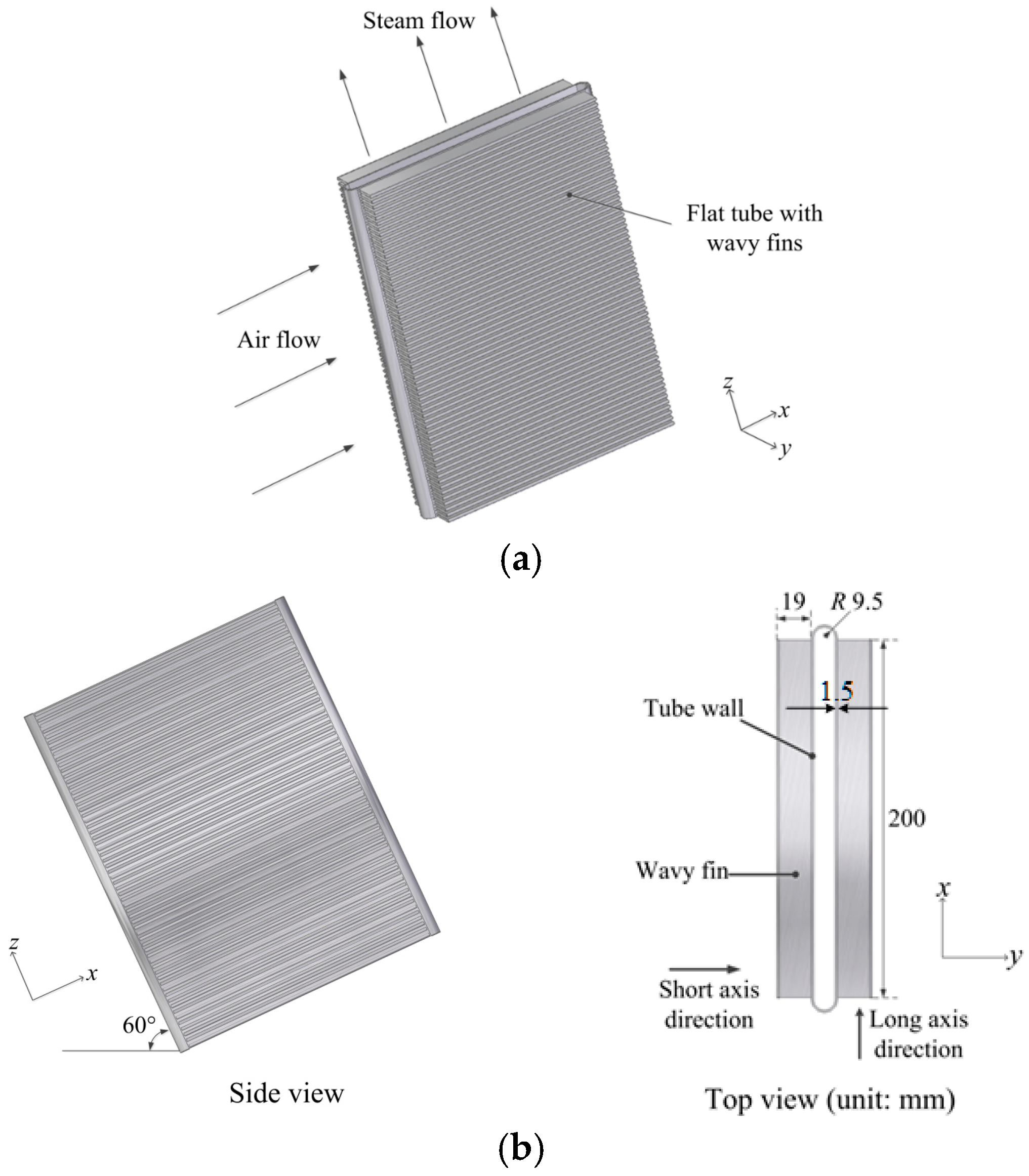
Figure 2.
(a) Computational domain of the finned flat tube; (b) Schematic of mesh; (c) The side view of finned flat tube.
Figure 2.
(a) Computational domain of the finned flat tube; (b) Schematic of mesh; (c) The side view of finned flat tube.
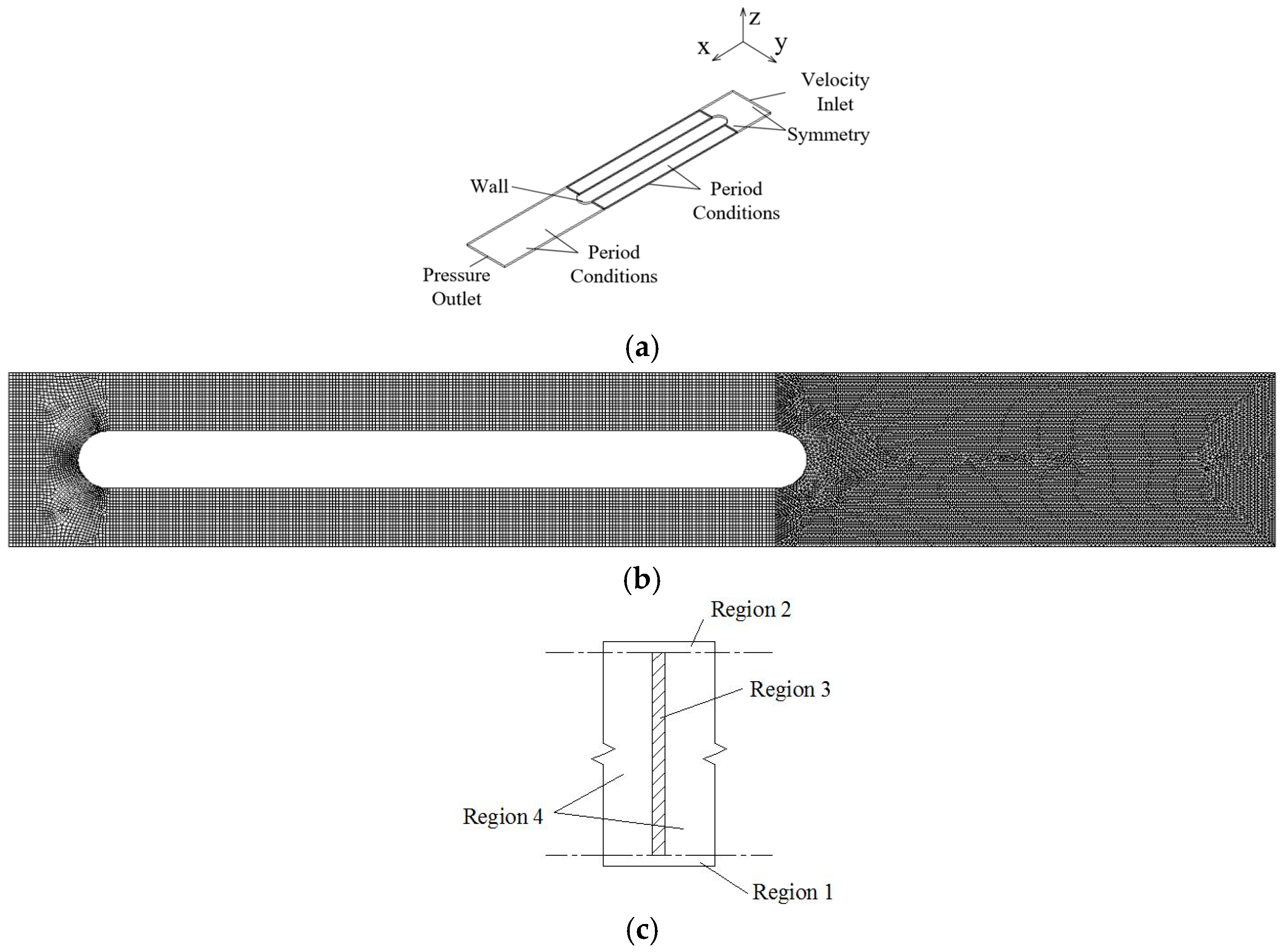
Figure 3.
The equivalent model for steam-side condensation of finned flat tube.

Figure 4.
Schematic diagram of control volume of condensate film on inner wall of flat tube.

Figure 5.
Integration of the backpressure and windward velocity.
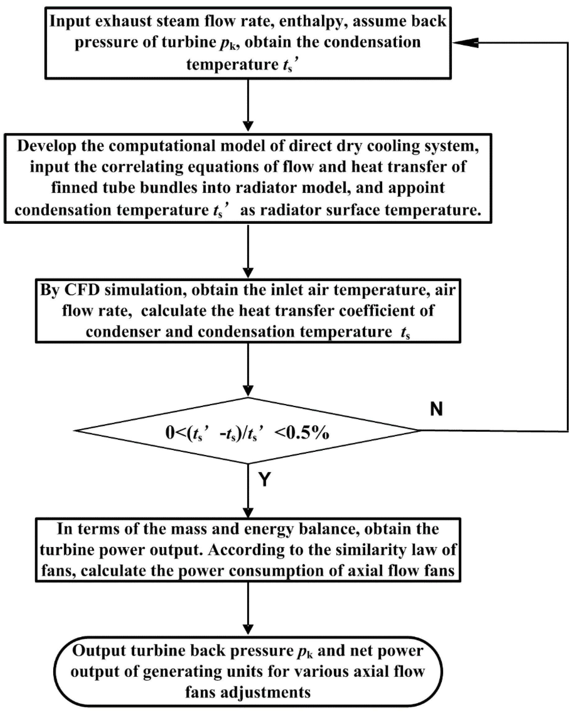
Figure 6.
Condensate film thickness on flat tube inner wall.

Figure 7.
Four representative condensation temperatures for finned flat tube.
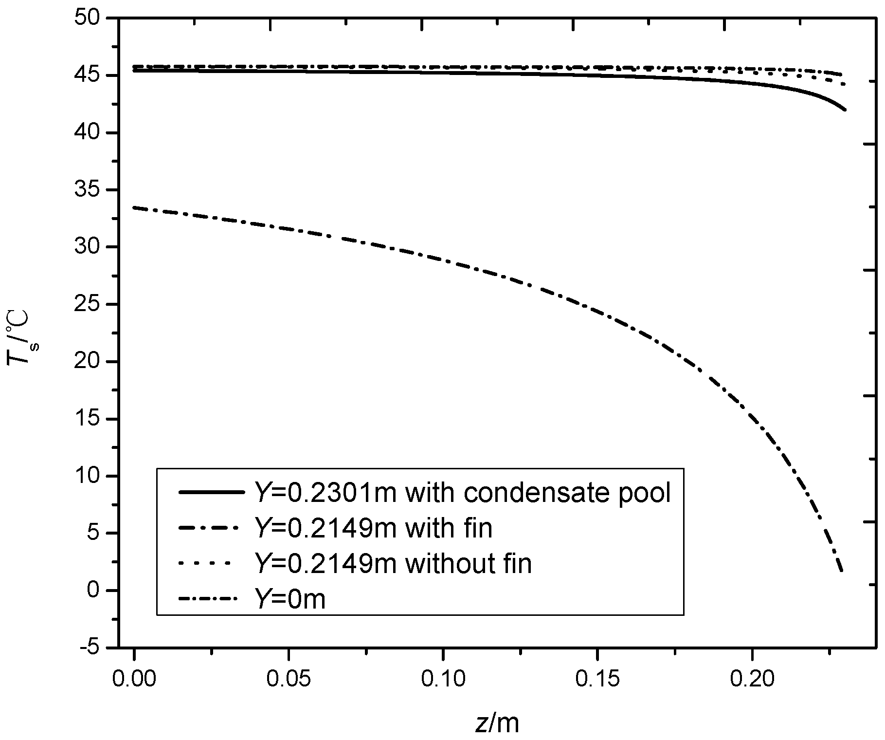
Figure 8.
(a) Average non-condensable gas concentration of tube section along tube length; (b) Condensation temperature at initial fin of flat tube along length.
Figure 8.
(a) Average non-condensable gas concentration of tube section along tube length; (b) Condensation temperature at initial fin of flat tube along length.
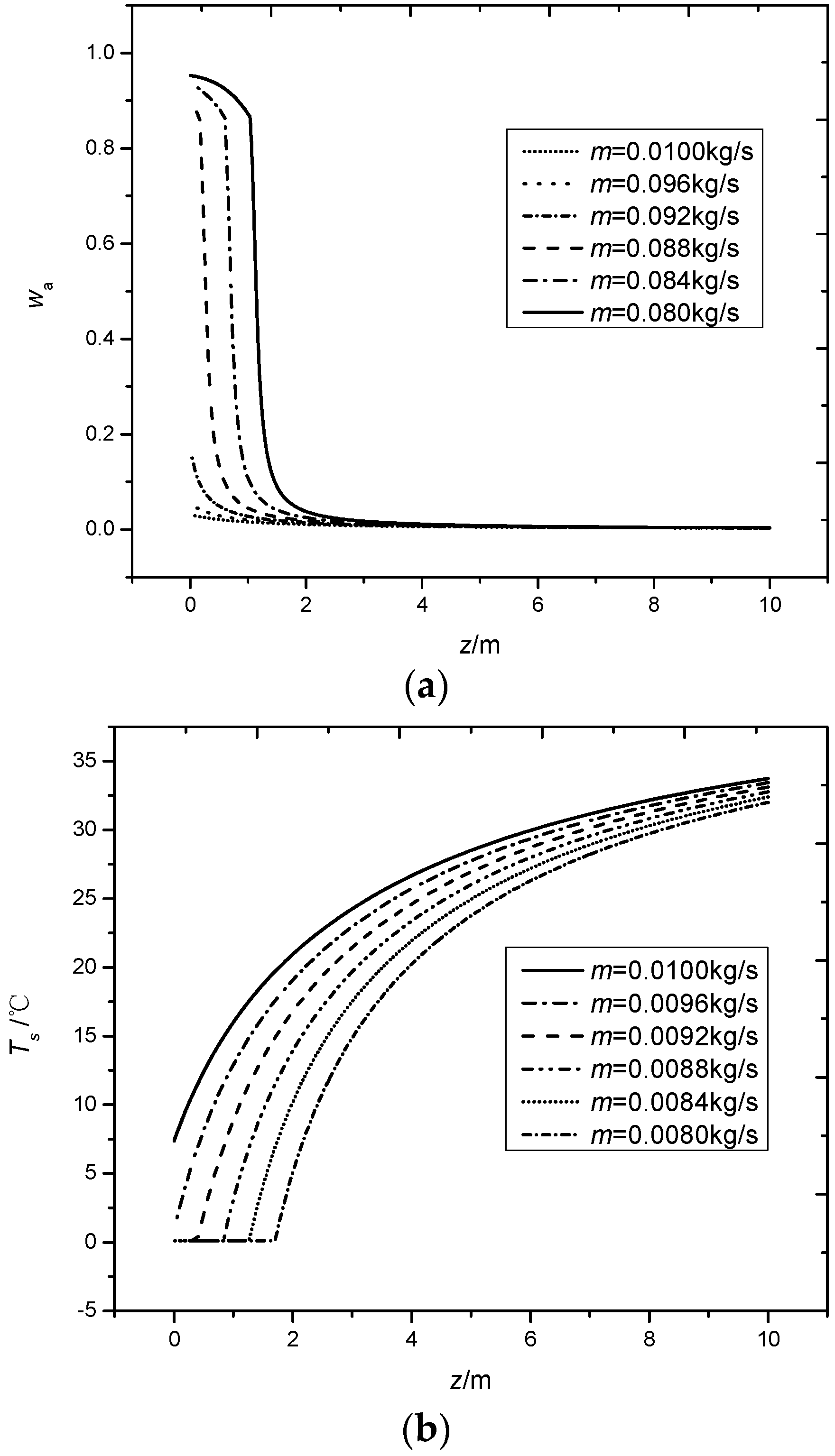
Figure 9.
(a) Critical freezing gas concentration versus inlet steam flow; (b) Critical freezing outlet flow versus inlet steam flow.
Figure 9.
(a) Critical freezing gas concentration versus inlet steam flow; (b) Critical freezing outlet flow versus inlet steam flow.
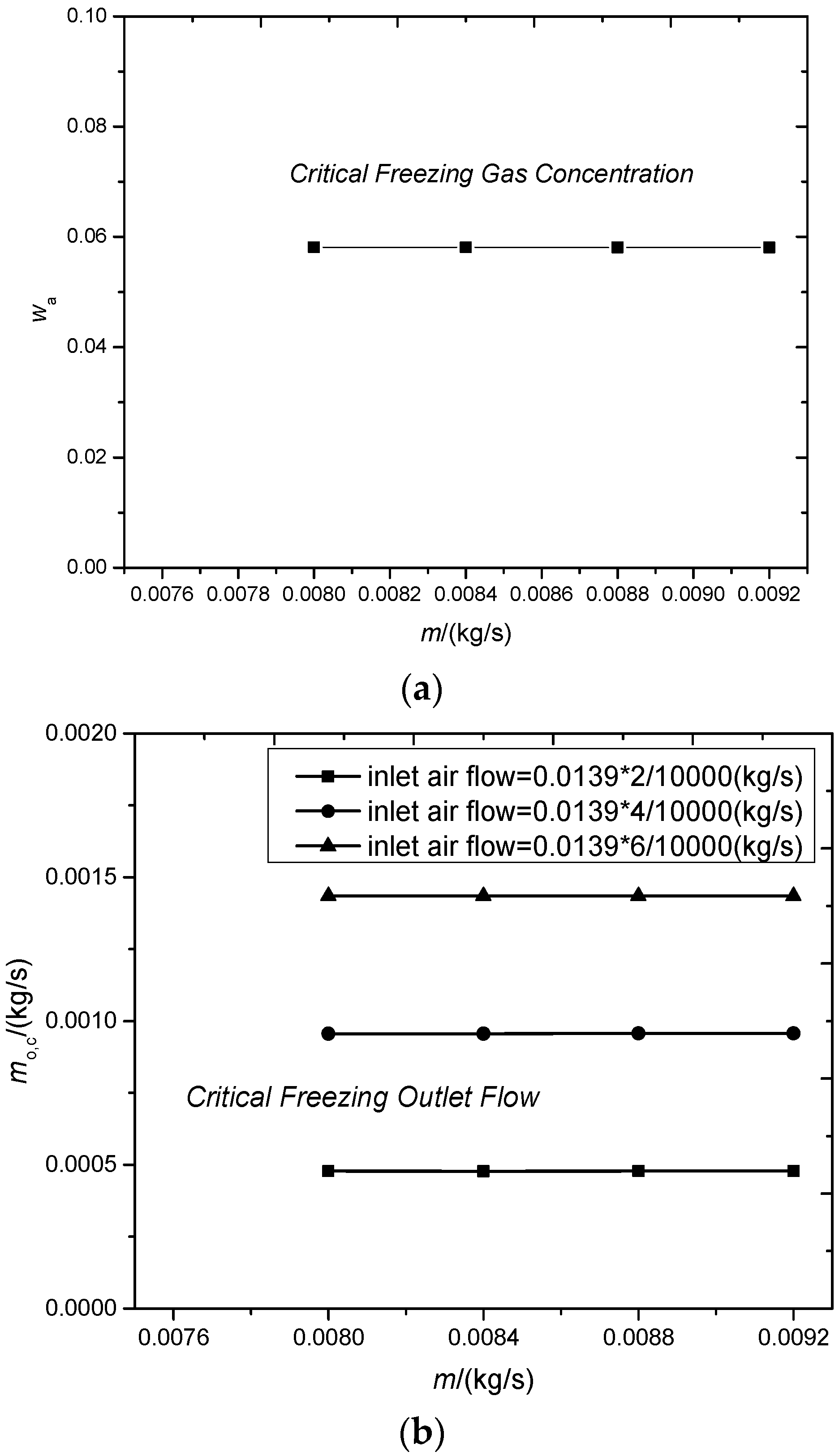
Figure 10.
Critical freezing outlet flow versus ambient temperature.
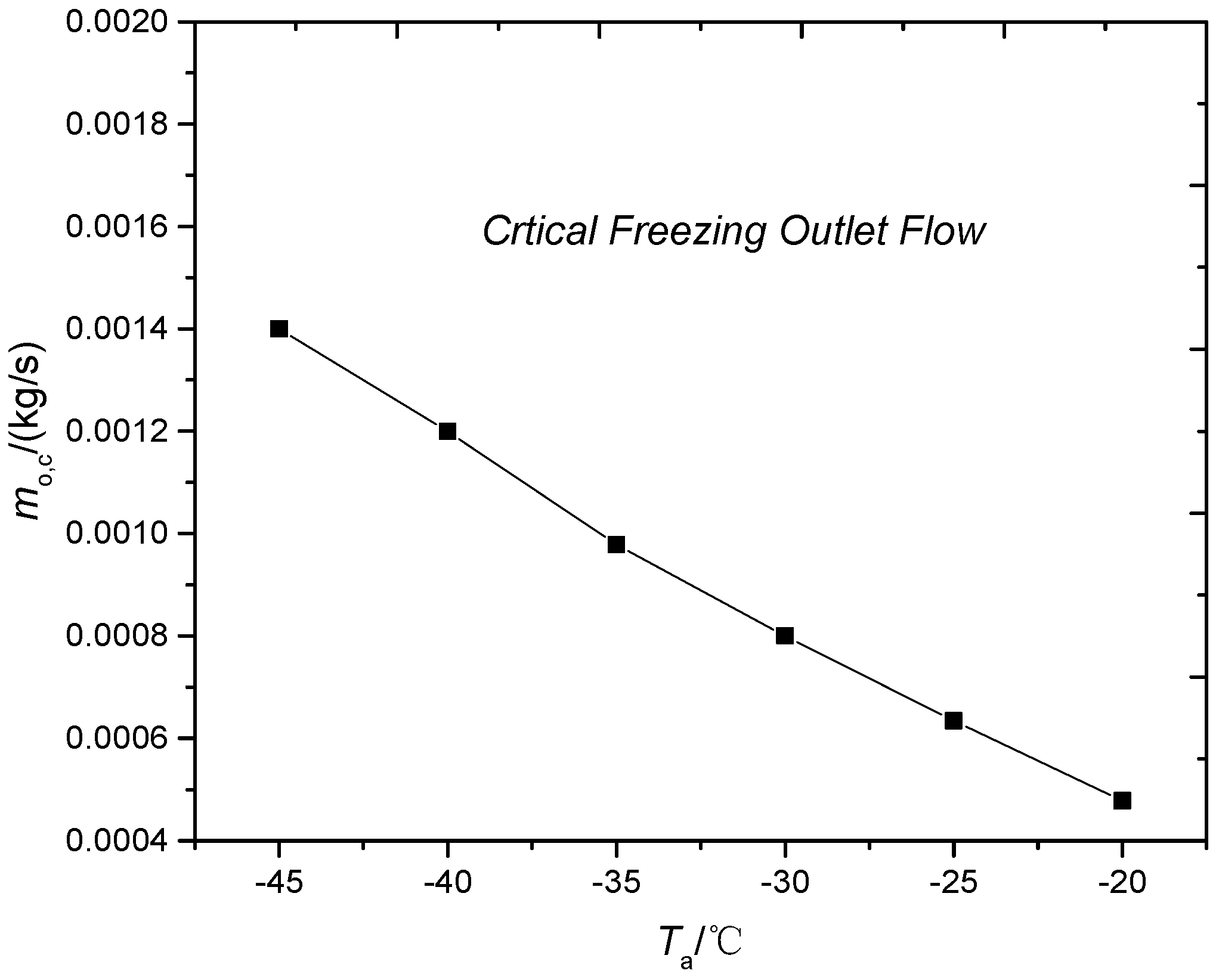
Figure 11.
Critical freezing outlet flow versus windward velocity.
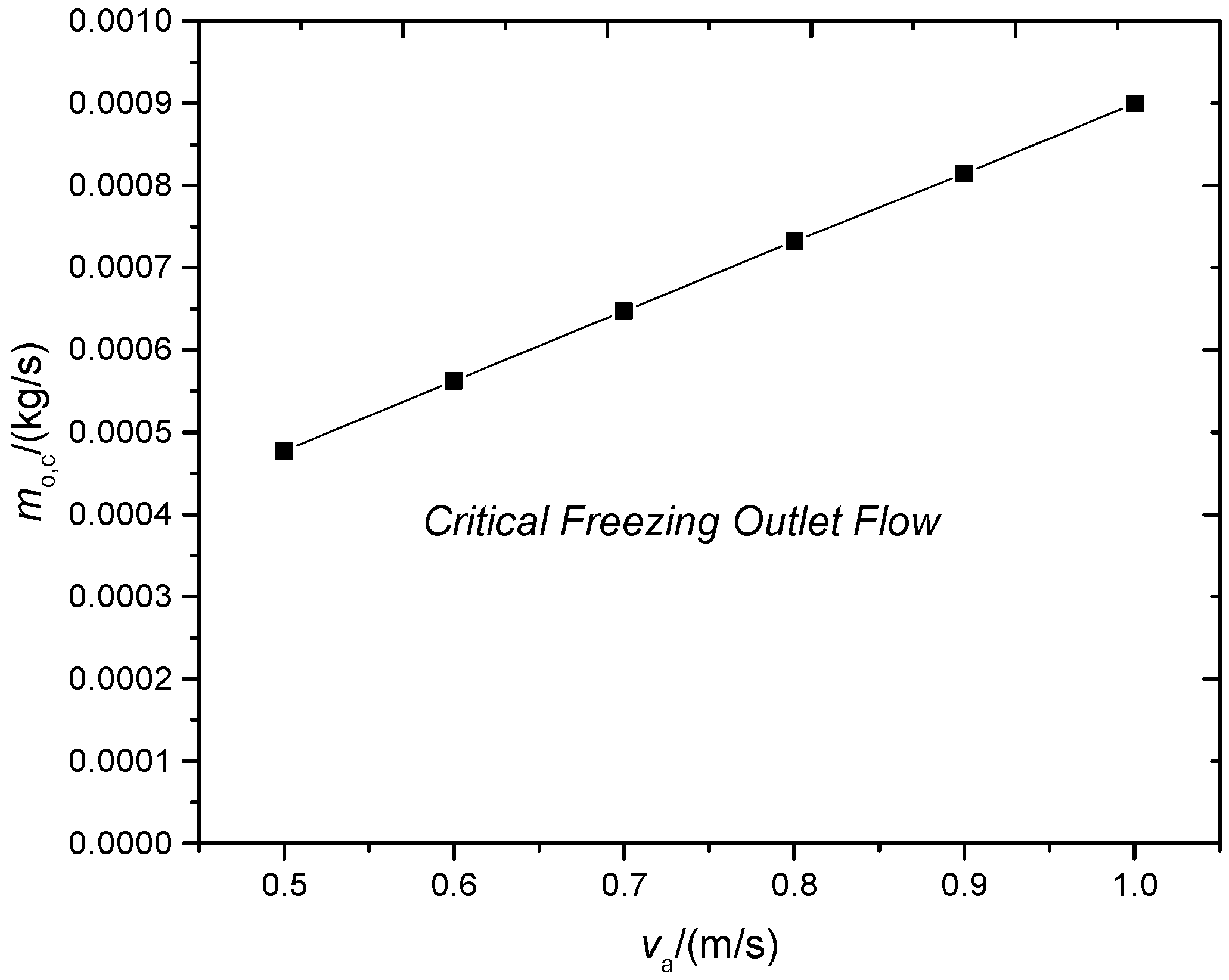
Figure 12.
Critical freezing outlet flow versus back pressure.

Figure 13.
Critical freezing outlet flow versus fin thickness.

Table 1.
Variation of critical freezing outlet flow.
| Variables | wa | Ta/°C | va/(m/s) | pc/kPa | δg/mm |
|---|---|---|---|---|---|
| Variable increment | 2.2/100,000 | 1 | 0.1 | 1 | 0.01 |
| Critical freezing outlet flow increment (kg/s) | 2.390 × 10⁻⁵ | 3.690 × 10⁻⁵ | 8.445 × 10⁻⁵ | 1.428 × 10⁻⁵ | 1.370 × 10⁻⁵ |
© 2017 by the authors. Licensee MDPI, Basel, Switzerland. This article is an open access article distributed under the terms and conditions of the Creative Commons Attribution (CC BY) license (http://creativecommons.org/licenses/by/4.0/).
Share and Cite
MDPI and ACS Style
Guo, Y.; Cheng, T.; Du, X.; Yang, L. Anti-Freezing Mechanism Analysis of a Finned Flat Tube in an Air-Cooled Condenser. Energies 2017, 10, 1872. https://doi.org/10.3390/en10111872
AMA Style
Guo Y, Cheng T, Du X, Yang L. Anti-Freezing Mechanism Analysis of a Finned Flat Tube in an Air-Cooled Condenser. Energies. 2017; 10(11):1872. https://doi.org/10.3390/en10111872
Chicago/Turabian StyleGuo, Yonghong, Tongrui Cheng, Xiaoze Du, and Lijun Yang. 2017. "Anti-Freezing Mechanism Analysis of a Finned Flat Tube in an Air-Cooled Condenser" Energies 10, no. 11: 1872. https://doi.org/10.3390/en10111872
Note that from the first issue of 2016, this journal uses article numbers instead of page numbers. See further details here.