Intelligent Energy Management Control for Extended Range Electric Vehicles Based on Dynamic Programming and Neural Network

Abstract
:1. Introduction
2. Optimization Problem and Formulation
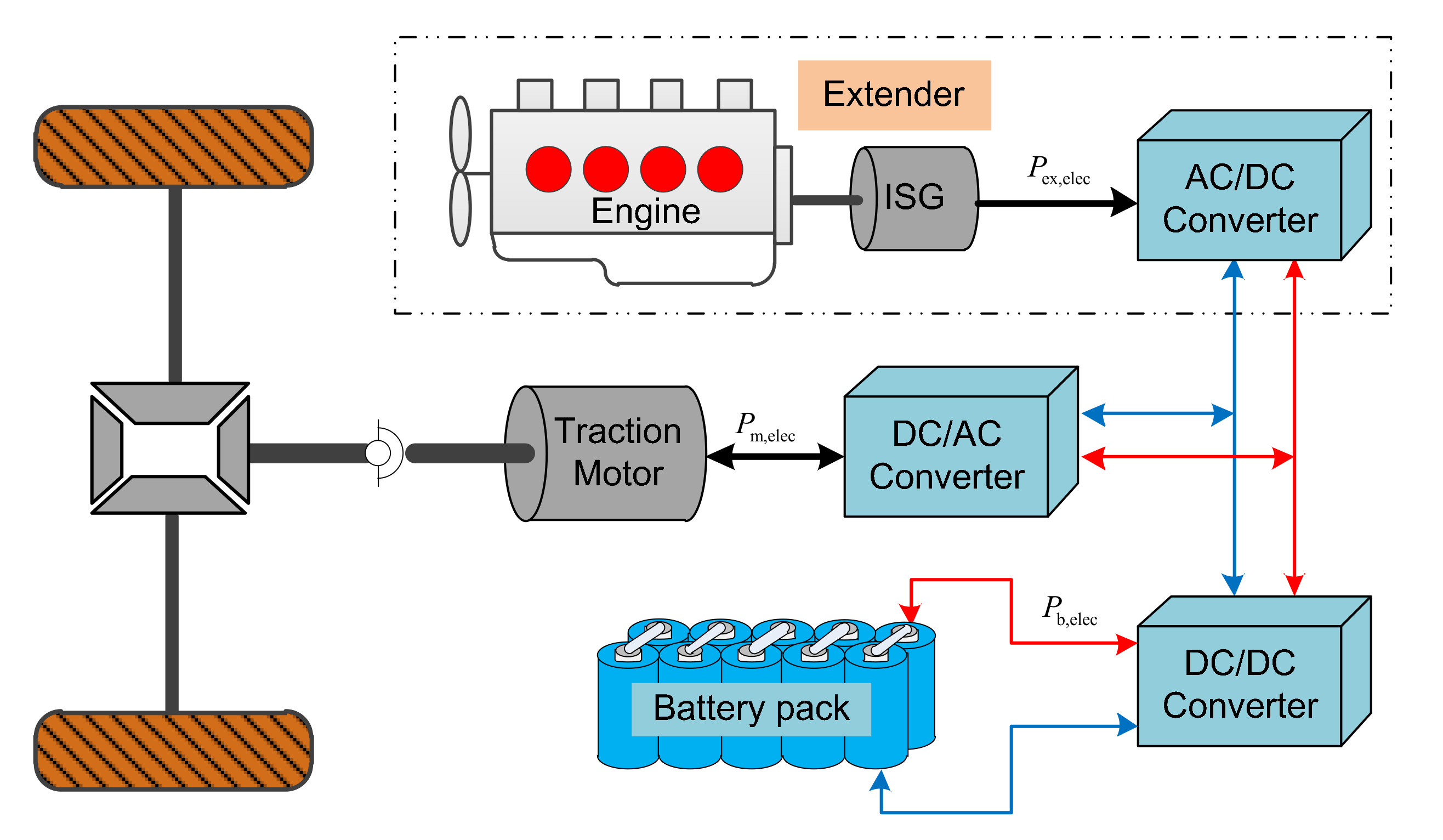
2.1. EREV Configuration
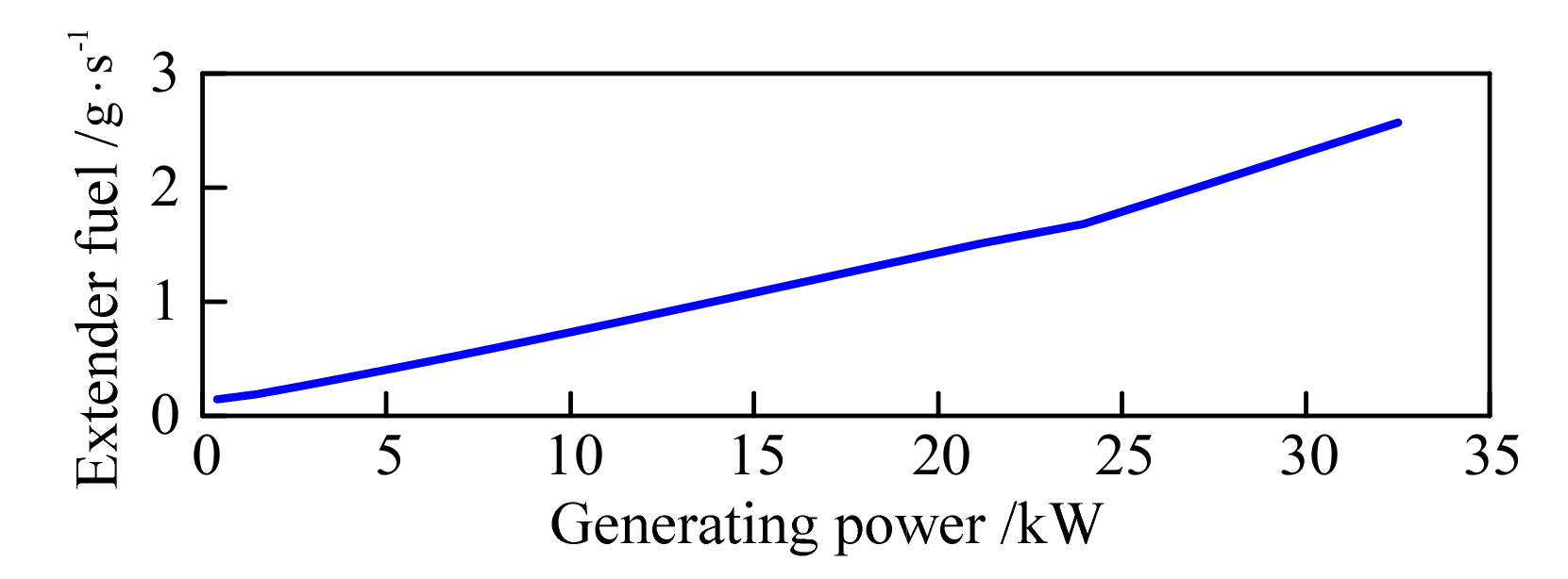
2.2. EREV Subsystem Model
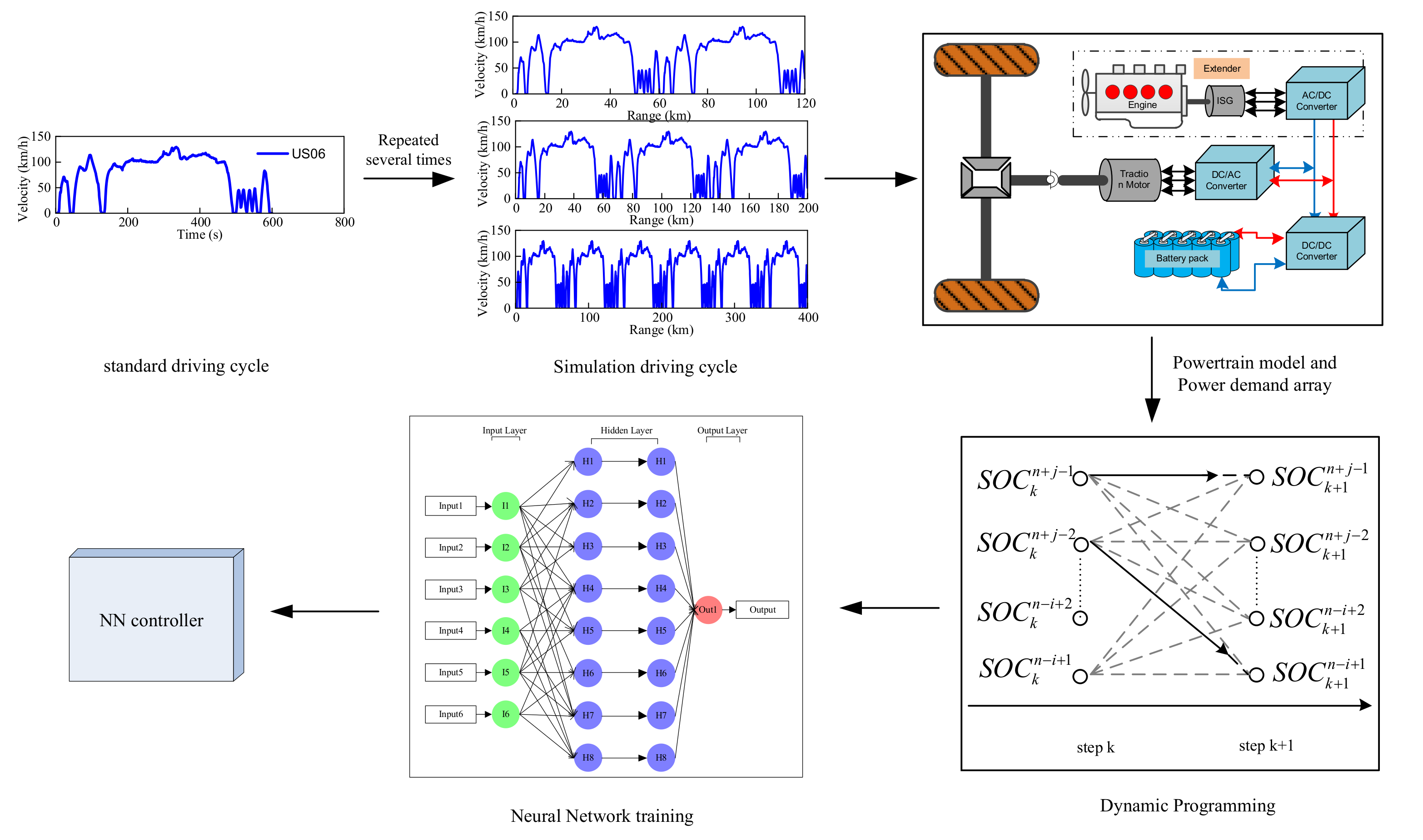
2.3. Dynamic Programming
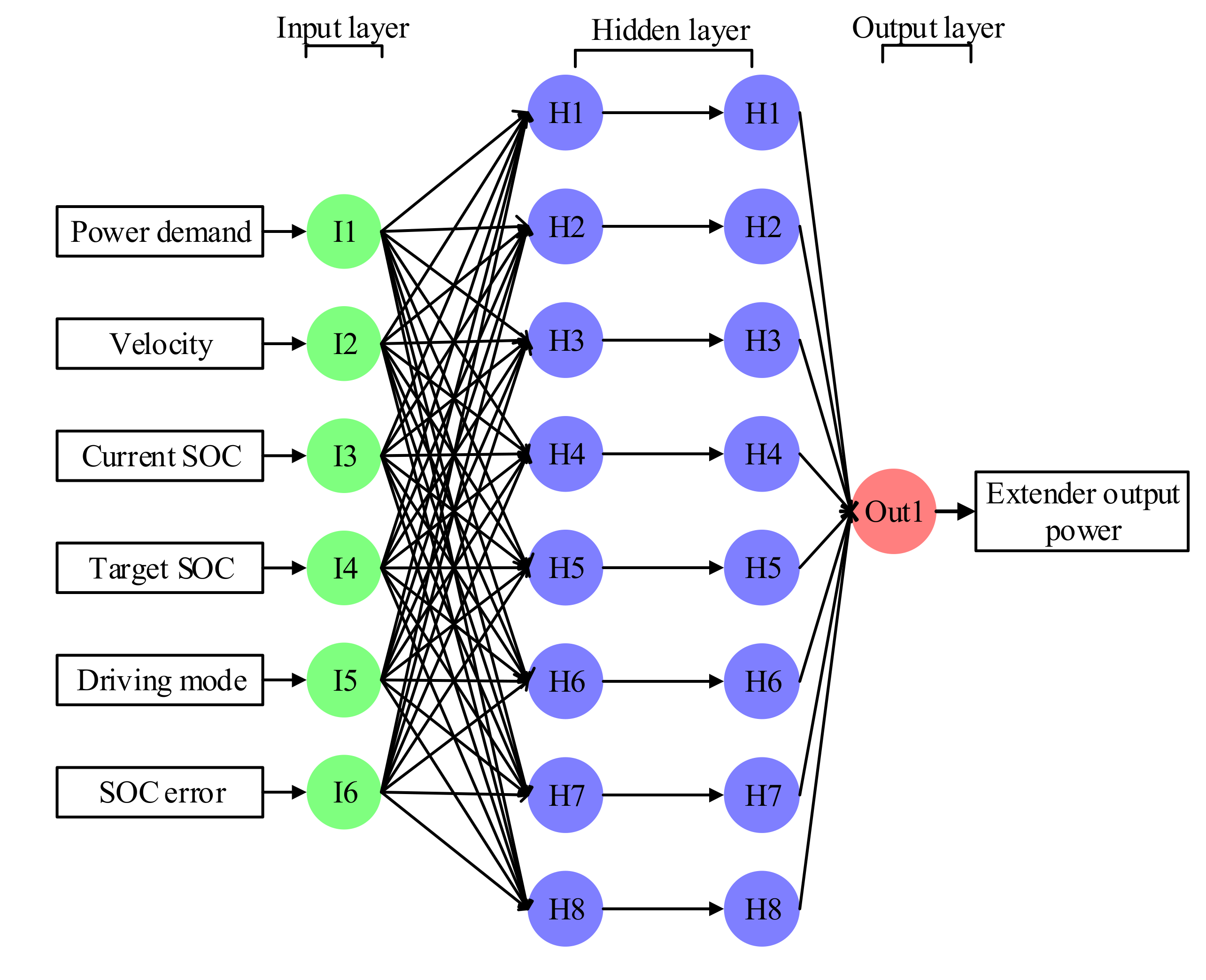
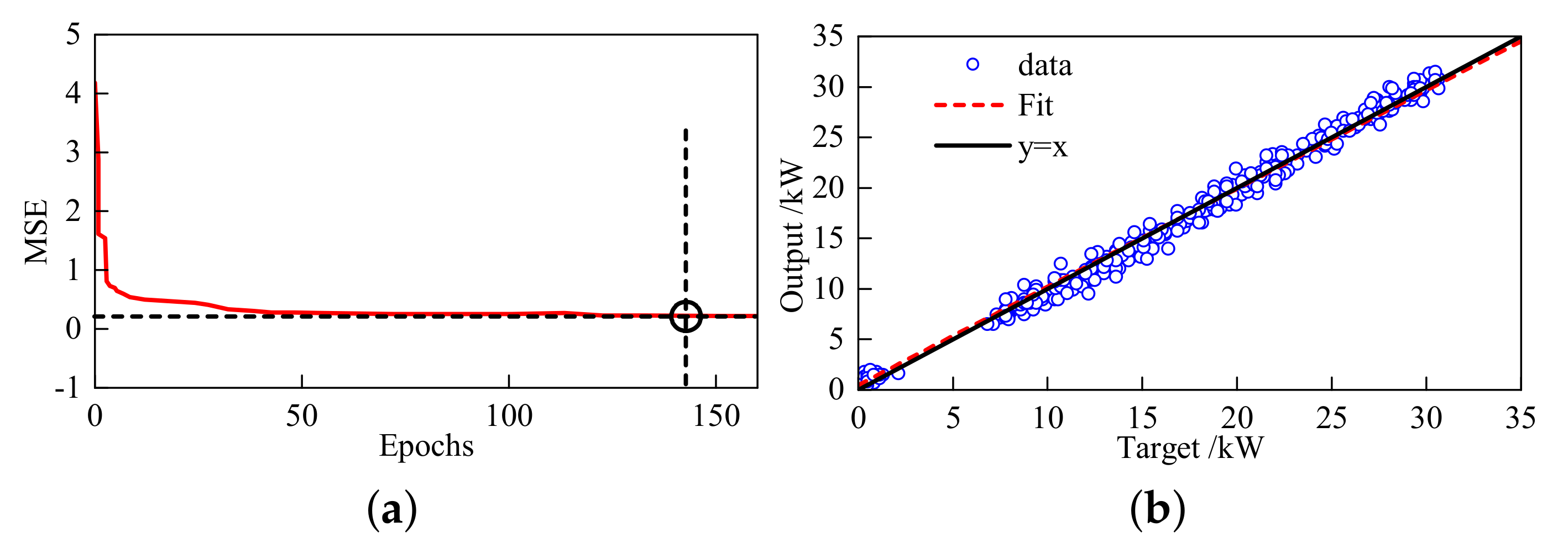
3. Neural Network Learning Optimal Control
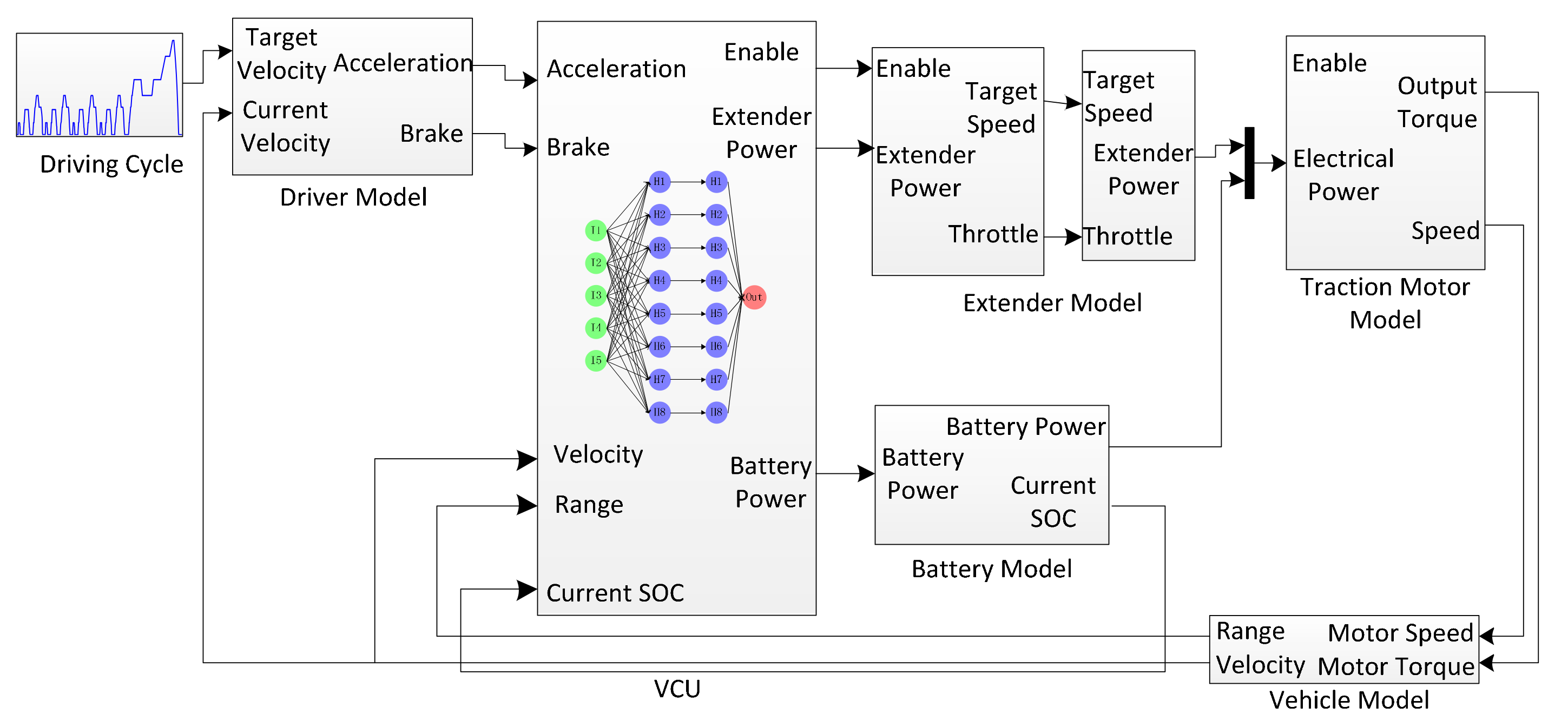
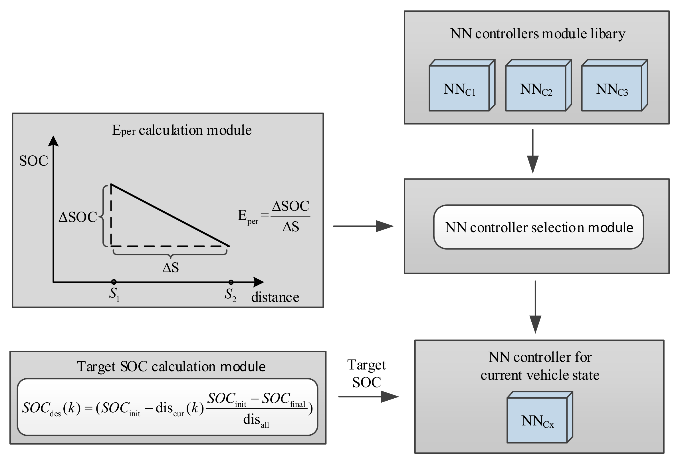
4. Intelligent Online Control
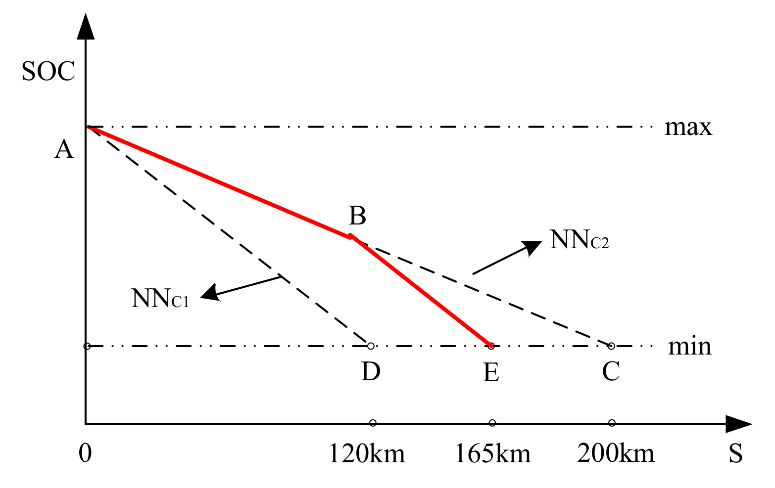
4.1. Controller Module Library
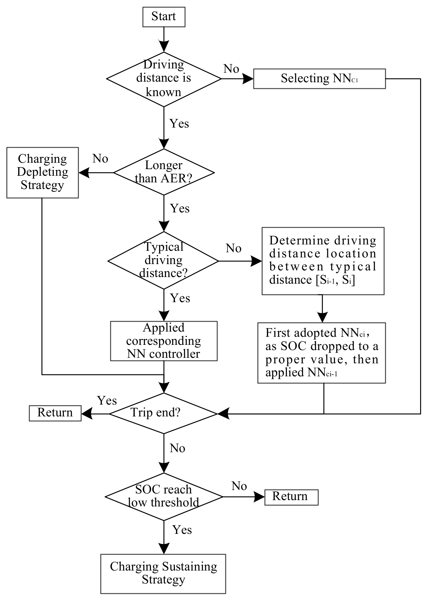
4.2. Intelligent Energy Management Controller
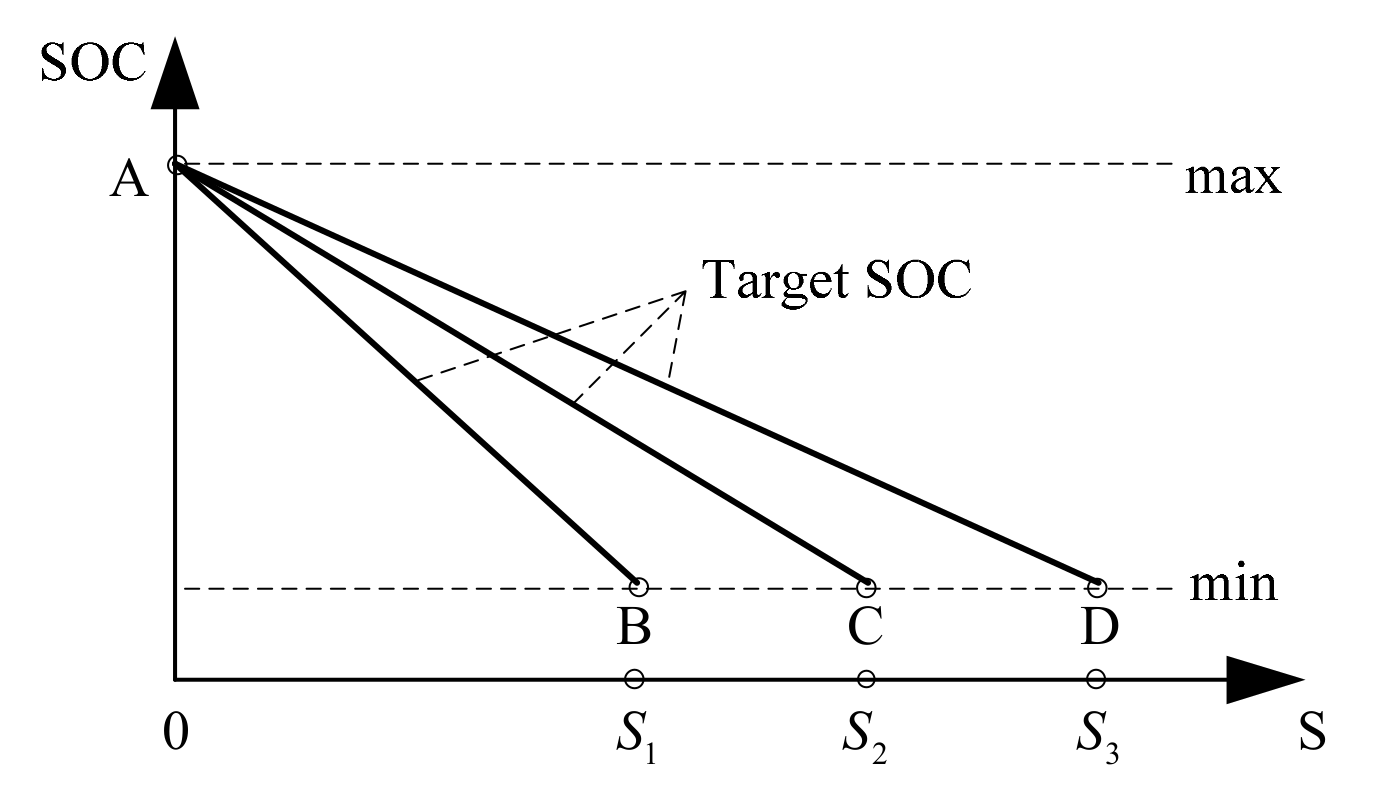
4.2.1. Electricity Consumption per Unit Distance Calculation Model
4.2.2. NN_Controller Selection Module
5. Simulation Results and Analysis
5.1. Simulation with Unknown Driving Distance
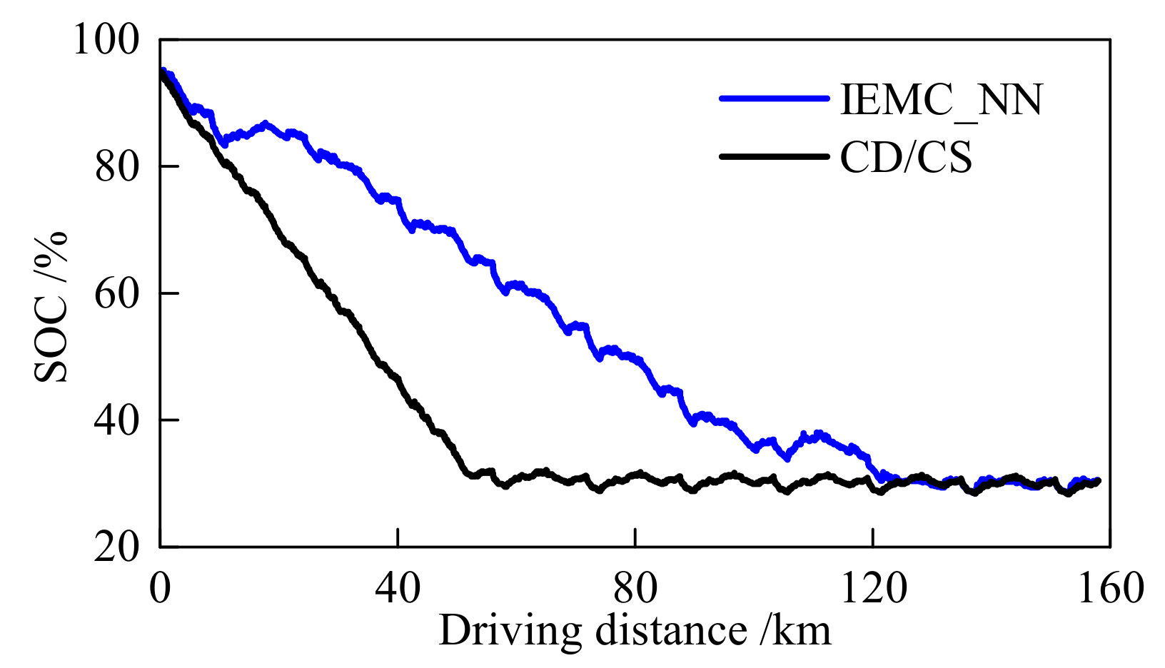
5.2. Simulation with a Normal Driving Distance
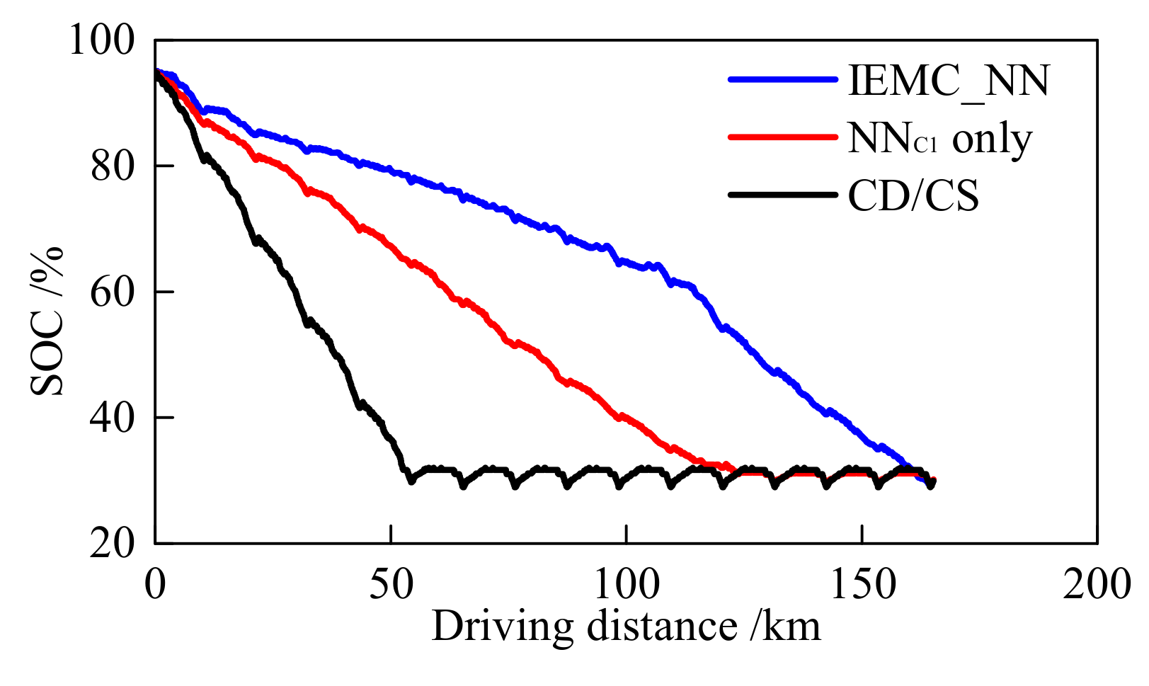
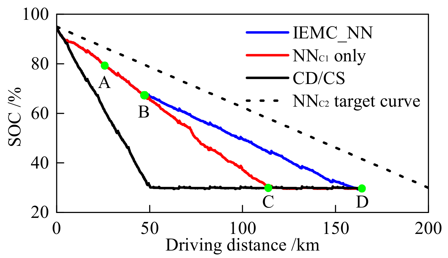
5.3. Simulation with a Changing Target Driving Distance during the Trip
6. Conclusions
Acknowledgments
Author Contributions
Conflicts of Interest
References
- Shi, X.Q.; Sun, Z.X.; Li, X.; Li, J.; Yang, J. A comparative study on environmental impacts of life cycle between electric taxi and fuel taxi in Beijing. Environ. Sci. 2015, 36, 1105–1116. [Google Scholar]
- Chen, Z.; Xiong, R.; Wang, K.; Jiao, B. Optimal energy management strategy of a plug-in hybrid electric vehicle based on a particle swarm optimization algorithm. Energies 2015, 8, 3661–3678. [Google Scholar] [CrossRef]
- Un-Noor, F.; Sanjeevikumar, P.; Mihet-Popa, L.; Mollah, M.N.; Hossain, E. A Comprehensive study of key electric vehicle (EV) components, technologies, challenges, impacts, and future direction of development. Energies 2017, 10, 1217. [Google Scholar] [CrossRef]
- Gu, Q.; Dou, F.; Ma, F. Energy optimal path planning of electric vehicle based on improved A* algorithm. Trans. Chin. Soc. Agric. Mach. 2015, 46, 316–322. [Google Scholar]
- Hall, J.; Marlok, H.; Bassett, H.; Warth, M. Analysis of real world data from a range extended electric vehicle demonstrator. SAE Int. J. Altern. Power. 2015, 4, 20–33. [Google Scholar] [CrossRef]
- Hong, S.; Wenjie, L.; Jing-Min, Y.; Yin-Ping, G. Optimization of energy management strategy for a Paralle-l series HEV. Trans. Chin. Soc. Agric. Mach. 2009, 40, 31–35. [Google Scholar]
- Fraidl, G.K.; Beste, F.; Kapus, P.E.; Korman, M.; Sifferlinger, B.; Vincen, B. Challenges and solutions for range extenders—From concept considerations to practical experiences. In Proceedings of the TO ZEV—Highlighting the Latest Powertrain, Vehicle and Infomobility Technologies, Turin, Italy, 9–10 June 2011. [Google Scholar]
- Škugor, B.; Cipek, M.; Deur, J. Control variables optimization and feedback control strategy design for the blended operating regime of an extended range electric vehicle. SAE Int. J. Altern. Power. 2014, 3, 152–162. [Google Scholar] [CrossRef]
- Song, W.; Zhang, X.; Tian, Y.; Xi, L. Driving pattern recognition and charging management-based intelligent control strategy for extended-range electric vehicles. J. Automot. Safety Energy 2016, 7, 224–229. [Google Scholar]
- Song, W.; Zhang, X.; Tian, Y.; Xi, L. A charging management-based intelligent control strategy for extended-range electric vehicles. J. Zhejiang Univ. Sci. A (Appl. Phys. Eng.) 2016, 17, 903–910. [Google Scholar]
- Wirasingha, S.G.; Emadi, A. Classification and review of control strategies for plug-in hybrid electric vehicles. In Proceedings of the Vehicle Power and Propulsion Conference (VPPC ’09), Dearborn, MI, USA, 7–10 September 2009; pp. 907–914. [Google Scholar]
- Du, J.; Chen, J.; Song, Z.; Gao, M.; Ouyang, M. Design method of a power management strategy for variable battery capacities range-extended electric vehicles to improve energy efficiency and cost-effectiveness. Energy 2017, 121, 32–42. [Google Scholar] [CrossRef]
- Xie, S.; Li, H.; Xin, Z.; Liu, T.; Wei, L. A pontryagin minimum principle-based adaptive equivalent consumption minimum strategy for a plug-in hybrid electric bus on a fixed route. Energies 2017, 10, 1379. [Google Scholar] [CrossRef]
- Patil, R.; Adornato, B.; Filipi, Z. Design optimization of a series plug-in hybrid electric vehicle for real-world driving conditions. SAE Int. J. Engines 2010, 3, 655–665. [Google Scholar] [CrossRef]
- Hai-tao, M.; Dong-jin, Y.; Yuan-bin, Y. Optimization of the control strategy for range extended electric vehicle. Automot. Eng. 2014, 36, 899–903. [Google Scholar]
- Banvait, H.; Anwar, S.; Chen, Y. A rule-based energy management strategy for plug-in hybrid electric vehicle (PHEV). In Proceedings of the American Control Conference (ACC’09), St. Louis, MO, USA, 10–12 June 2009; pp. 3938–3943. [Google Scholar]
- Rousseau, A.; Pagerit, S.; Gao, D.W. Plug-in hybrid electric vehicle control strategy parameter optimization. J. Asian Electr. Veh. 2008, 6, 1125–1133. [Google Scholar] [CrossRef]
- Schacht, E.; Bezaire, B.; Cooley, B.; Bayar, K.; Kruckenberg, J.W. Addressing drivability in an extended range electric vehicle running an equivalent consumption minimization strategy. In Proceedings of the SAE 2011 World Congress & Exhibition, Detroit, MI, USA, 12–14 August 2011. [Google Scholar]
- Waldner, J.; Wise, J.; Crawford, C.; Dong, Z. Development and testing of an advanced extended range electric vehicle. In Proceedings of the SAE 2011 World Congress & Exhibition, Detroit, MI, USA, 12–14 August 2011. [Google Scholar]
- Sharer, P.B.; Rousseau, A.; Karbowski, D.; Pagerit, S. Plug-in Hybrid Electric Vehicle Control Strategy: Comparison between EV and Charge-Depleting Options; SAE Technical Paper 2008-01-0460; SAE International: Warrendale, PA, USA; Troy, MI, USA, 2008. [Google Scholar]
- Chen, B.C.; Wu, Y.Y.; Tsai, H.C. Design and analysis of power management strategy for range extended electric vehicle using dynamic programming. Appl. Energy 2014, 113, 1764–1774. [Google Scholar] [CrossRef]
- Chen, Z.; Mi, C.C.; Xu, J.; Gong, X.; You, C. Energy management for a power-split plug-in hybrid electric vehicle based on dynamic programming and neural networks. IEEE Trans. Veh. Technol. 2014, 63, 1567–1580. [Google Scholar] [CrossRef]
- Murphey, Y.L.; Park, J.; Chen, Z.; Kuang, M.L.; Masrur, M.A.; Phillips, A.M. Intelligent hybrid vehicle power control—Part I: Machine learning of optimal vehicle power. IEEE Trans. Veh. Technol. 2012, 61, 3519–3530. [Google Scholar] [CrossRef]
- Murphey, Y.L.; Park, J.; Chen, Z.; Kuang, M.L.; Masrur, M.A.; Phillips, A.M. Intelligent hybrid vehicle power control—Part II: Online intelligent energy management. IEEE Trans. Veh. Technol. 2013, 62, 69–79. [Google Scholar] [CrossRef]
- Zhou, W.; Zhang, C.; Li, J. Analysis and comparison of optimal power management strategies for a series plug-in hybrid school bus via dynamic programming. INT. J. Vehicle. Des. 2015, 69, 113–131. [Google Scholar] [CrossRef]
- Karbowski, D.; Rousseau, A.; Pagerit, S.; Sharer, P. Plug-in vehicle control strategy: From global optimization to real-time application. In Proceedings of the 22nd electric vehicle symposium, EVS22, Yokohama, Japan, 25 October 2006. [Google Scholar]
- Patil, R.M.; Filipi, Z.; Fathy, H.K. Comparison of supervisory control strategies for series plug-in hybrid electric vehicle powertrains through dynamic programming. IEEE Trans. Contr. Syst. Technol. 2014, 22, 502–509. [Google Scholar] [CrossRef]
- Yu, Z. Automobile Theory; China Machine Press: Beijing, China, 2009. [Google Scholar]
- Bellman, R.E.; Dreyfus, S.E. Applied Dynamic Programming; Princeton University Press: Princeton, NJ, USA, 1962. [Google Scholar]
- Sundström, O.; Ambühl, D.; Guzzella, L. On implementation of dynamic programming for optimal control problems with final state constraints. Oil Gas Sci. Technol. 2009, 65, 91–102. [Google Scholar] [CrossRef]
- Wang, X.; He, H.; Sun, F.; Zhang, J. Application study on the dynamic programming algorithm for energy management of plug-in hybrid electric vehicles. Energies 2015, 8, 3225–3244. [Google Scholar] [CrossRef]
- Zou, Y.; Hou, S.; Han, E.; Liu, L.; Chen, R. Dynamic programming-based energy management strategy optimization for hybrid electric commercial vehicle. Automot. Eng. 2012, 34, 663–668. [Google Scholar]
- Lin, C.C.; Peng, H.; Jeon, S.; Jang, M.L. Control of a hybrid electric truck based on driving pattern recognition. In Proceedings of the 2002 Advanced Vehicle Control Conference, Hiro Shima, Japan, 9–13 September 2002; pp. 41–58. [Google Scholar]
- Park, J.; Chen, Z.; Kiliaris, L.; Kuang, M.L.; Masrur, M.A.; Phillips, A.M.; Murphey, Y.L. Intelligent vehicle power control based on machine learning of optimal control parameters and prediction of road type and traffic congestion. IEEE Trans. Veh. Technol. 2009, 58, 4741–4756. [Google Scholar] [CrossRef]
- Beijing Daily. Using Intensity Too High Need to Be Guided, Tong Xin Press: Beijing, China, 2011.
- Niu, J.; Si, L.; Zhou, S.; Zhang, T. Simulation analysis of energy control strategy for an extended-range electric vehicle. J. Shanghai Jiaotong Univ. 2014, 48, 140–145. [Google Scholar] [CrossRef]


| Components | Parameters | Values |
|---|---|---|
| Engine | Displacement/L | 0.9 |
| Maximum power/kW | 52 | |
| Maximum torque/Nm | 90 | |
| Generator | Maximum power/kW | 53 |
| Maximum torque/Nm | 155 | |
| Traction motor | Maximum power/kW | 130 |
| Maximum torque/Nm | 480 | |
| Power Battery | Capacity/Ah | 37 |
| Voltage/V | 360 | |
| Others | Final drive ratio | 7.793 |
| Curb mass/kg | 1400 | |
| Front area/m | 2.9 | |
| Tire rolling radius/m | 0.298 | |
| Transmission efficiency/% | 92 |
| Layer | Parameters | Accuracy |
|---|---|---|
| Power demand/kw | 0.1 | |
| Velocity/km·h | 0.01 | |
| Current SOC/% | 0.1 | |
| Input layer | Target SOC/% | 0.1 |
| SOC error/% | 0.1 | |
| Driving trend | 1 | |
| Output layer | Extender output power/kw | 0.1 |
| Controller | Duration/s | Target Driving Distance/km | Fuel Consumption/L | Final SOC/% | Saving Rate/% |
|---|---|---|---|---|---|
| CD/CS | 14360 | 158 | 6.36 | 30.5 | - |
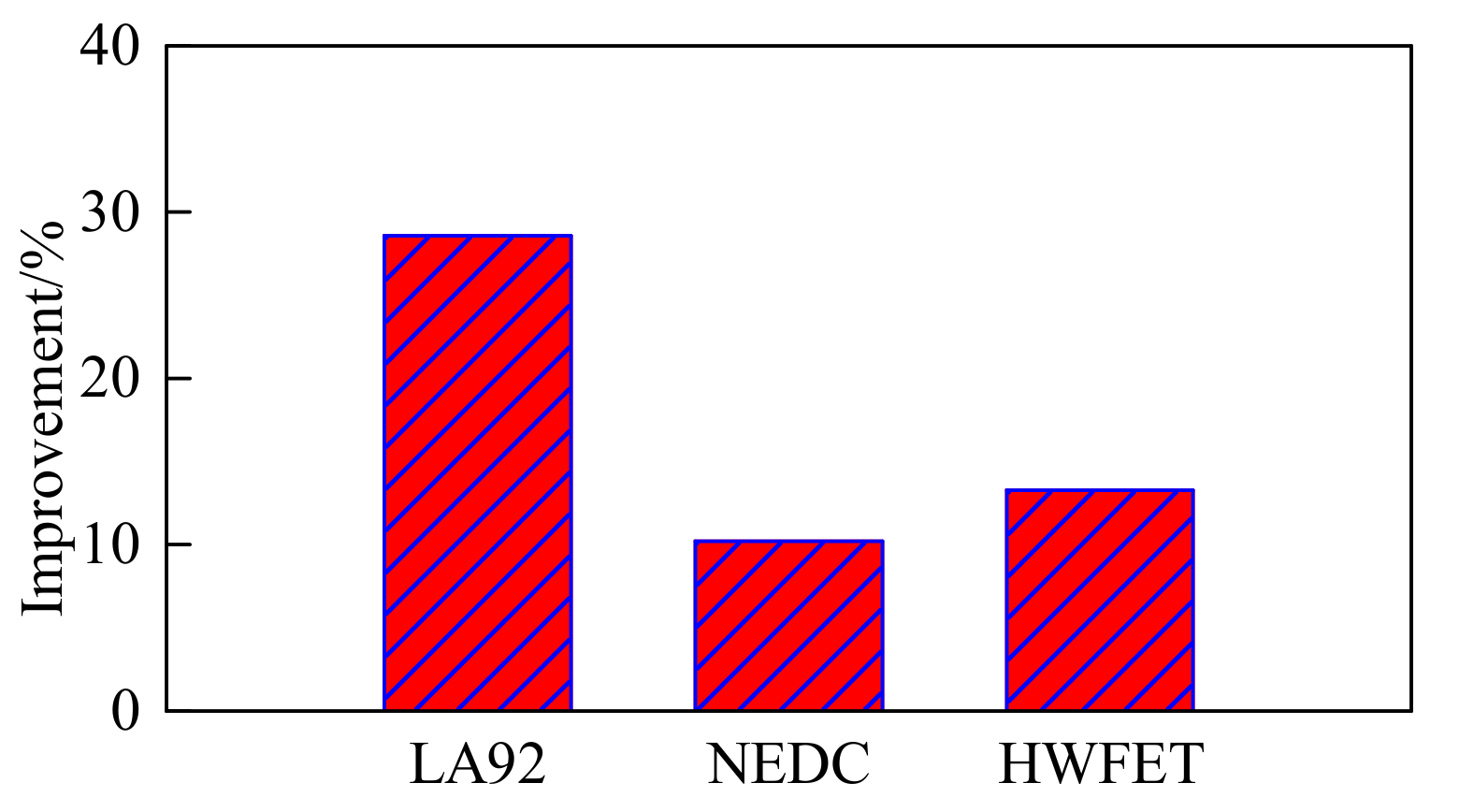
| IEMC_NN | 14360 | 158 | 4.54 | 30.5 | 28.6 |
| Controller | Duration/s | Target Driving Distance/km | Fuel Consumption/L | Final SOC/% | Saving Rate/% |
|---|---|---|---|---|---|
| CD/CS | 17699 | 165 | 5.22 | 29.5 | - |
| NN only | 17699 | 165 | 4.87 | 30.2 | 6.7 |
| IEMC_NN | 17699 | 165 | 4.77 | 31.5 | 10.2 |
| Controller | Duration/s | Target Driving Distance/km | Fuel Consumption/L | Final SOC/% | Saving Rate/% |
|---|---|---|---|---|---|
| CD/CS | 7660 | 165 km | 7.29 | 30.5 | - |
| NN only | 7660 | 165 km | 6.86 | 30.5 | 5.9 |
| IEMC_NN | 7660 | 165 km | 6.32 | 30.0 | 13.3 |
© 2017 by the authors. Licensee MDPI, Basel, Switzerland. This article is an open access article distributed under the terms and conditions of the Creative Commons Attribution (CC BY) license (http://creativecommons.org/licenses/by/4.0/).
Share and Cite
Xi, L.; Zhang, X.; Sun, C.; Wang, Z.; Hou, X.; Zhang, J. Intelligent Energy Management Control for Extended Range Electric Vehicles Based on Dynamic Programming and Neural Network. Energies 2017, 10, 1871. https://doi.org/10.3390/en10111871
Xi L, Zhang X, Sun C, Wang Z, Hou X, Zhang J. Intelligent Energy Management Control for Extended Range Electric Vehicles Based on Dynamic Programming and Neural Network. Energies. 2017; 10(11):1871. https://doi.org/10.3390/en10111871
Chicago/Turabian StyleXi, Lihe, Xin Zhang, Chuanyang Sun, Zexing Wang, Xiaosen Hou, and Jibao Zhang. 2017. "Intelligent Energy Management Control for Extended Range Electric Vehicles Based on Dynamic Programming and Neural Network" Energies 10, no. 11: 1871. https://doi.org/10.3390/en10111871