Applications of the Chaotic Quantum Genetic Algorithm with Support Vector Regression in Load Forecasting

1
Department of International Business, Chung Yuan Christian University, 200 Chung Pei Rd., Chungli District, Taoyuan City 32023, Taiwan
2
Ph.D. Program in Business, College of Business, Chung Yuan Christian University, 200 Chung Pei Rd., Chungli District, Taoyuan City 32023, Taiwan
*
Author to whom correspondence should be addressed.
Energies 2017, 10(11), 1832; https://doi.org/10.3390/en10111832
Submission received: 20 October 2017
/
Revised: 7 November 2017
/
Accepted: 8 November 2017
/
Published: 10 November 2017
(This article belongs to the Special Issue Hybrid Advanced Optimization Methods with Evolutionary Computation Techniques in Energy Forecasting)
Abstract
:Accurate electricity forecasting is still the critical issue in many energy management fields. The applications of hybrid novel algorithms with support vector regression (SVR) models to overcome the premature convergence problem and improve forecasting accuracy levels also deserve to be widely explored. This paper applies chaotic function and quantum computing concepts to address the embedded drawbacks including crossover and mutation operations of genetic algorithms. Then, this paper proposes a novel electricity load forecasting model by hybridizing chaotic function and quantum computing with GA in an SVR model (named SVRCQGA) to achieve more satisfactory forecasting accuracy levels. Experimental examples demonstrate that the proposed SVRCQGA model is superior to other competitive models.
1. Introduction
With rapid economic development, accurate electricity load forecasting has become essential for many energy applications, such as energy generation, power system operation security, load unit commitment, and energy marketing. For example, power system decision makers can optimize load dispatch and adjust the electricity supply/price based on the forecasted loads, i.e., improve the power system management efficiency. As indicated in Xiao et al. [1], in China, there would be a year-long operational benefit with a 1% increase in the forecasting accuracy level. In addition, accurate load forecasting could also help managers set up well electrical power scheduling and successfully reduce system management risks. On the customer side, accurate load forecasting also facilitates the power usage decisions of customers to avoid load usage during the peak times and paying higher electricity prices. This usage balance between peak and bottom periods would lead to reliable power system operation of a utility. On the contrary, inaccurate forecast results would lead to inefficient power system operations and increased operating costs. As mentioned in the literature, a 1% increase in load forecasting error can lead to a loss of millions of dollars [2]. Therefore, as electricity prices also play a critical role in electricity production decisions, there are also several scholars who have proposed electricity price forecasting models in the literature [3,4]. Readers may refer to Weron [5] for more comprehensive overviews.
The electricity load data are influenced by lots of factors, such as socio-economical activities, population, weather conditions, holidays, policy, and so on [6]. Therefore, the electric load data reveal nonlinearity, seasonality, and chaos in nature, so finding a robust load forecasting model with superior performance would be an important issue in the power load management field.
Researchers have developed and proposed lots of electricity load forecasting models. These forecasting models are often classified into two categories: traditional statistical models and artificial intelligence models. The first one are also called stochastic time series approach models, i.e., only historical data is used, which is easily to apply. These various famous time series models include the well-known Box–Jenkins’ ARIMA models [7], regression models [8], exponential smoothing models [9], Kalman filtering models [10], Bayesian estimation models [11], and so on. However, the embedded drawbacks of those models are that they are defined theoretically to deal with linear relationships among electricity load and other stochastic factors such as socio-economical activities and policy effects, thus, they have difficulties to effectively capture the complicate nonlinear relationships among load data and these factors, eventually, producing high unpredictable load forecasting performance errors [12].
The artificial intelligence models such as artificial neural networks (ANNs) [12], expert system models [13], and fuzzy methodologies [14] have been well explored to improve the accuracy of load forecasting since the 1980s. In recent years, the development of artificial intelligence approaches has focused on novel hybrid or combined models, obtained by hybridizing or combining these models with each other [15], with traditional statistical tools [16], and with superior evolutionary algorithms [17]. However, similarly, these artificial intelligence models also suffer from some shortcomings during the modeling processes, such as the fact they are very dependent on the collected data, and often are unstable. Thus, it is difficult to determine the network structural parameters [18]. It is also time consuming to extract knowledge from data sets [19], and they are easily trapped in local minima [20], for more insightful discussions of AI approaches in load forecasting readers may refer to [21].
Due to the superiority in modeling nonlinear data by mapping into the high dimensional feature space, support vector regression (SVR) [22] has been applied to solve forecasting issues many research fields in the late 1990s. For load forecasting problems, Hong [23,24] proposed a valuable series exploration by integrating advanced algorithms and chaotic function with an SVR-based model to determine its three parameters, and thus achieved satisfactory forecasting performance. According to Hong’s series research conclusions, good determination of parameters for the SVR model is important to achieve high forecasting accuracy levels and overcome the drawbacks of the hybrid evolutionary algorithms, such as becoming trapped in local optima, and this will ensure achieving more suitable parameter combinations. In the meanwhile, Bhunia [25] indicated that quantum computing principles can be embedded in intelligent systems to improve their performance; moreover, Dey et al. [26] also concluded that the use of both of quantum approaches and soft computing techniques in a combined form can provide a new computer science and engineering paradigm. Huang [27] proposed a novel forecasting model by hybridizing a chaotic function and a quantum PSO algorithm to receive higher forecast accuracy levels. Recently, Lee and Lin [28] also applied quantum concepts to propose the hybrid tabu search algorithm with the SVR model to adjust the three parameters and eventually obtain more accurate load forecasting performances.
The genetic algorithm (GA) is a famous algorithm which generates new offspring by finite iterative operations, including selection, crossover, mutation, and so on. It has attracted lots of attention to find satisfactory solutions and is applied in many fields. However, along with the increase of the data scale and more complicated problem, it often suffers from similar problem of becoming trapped in local optima and slow convergence to the global optimum. Dey et al. [26] claimed that an efficient quantum-based GA can be modeled to solve NP-hard problems and others. To continue exploring the feasibility of hybrid quantum-behaved approaches with advanced algorithms, and to overcome the embedded drawbacks of genetic algorithm mentioned above, this paper would like to apply quantum computing concepts to propose hybridizing chaotic function and quantum GA (namely CQGA) with the SVR model, creating the so-called SVRCQGA model to achieve more satisfactory load forecasting accuracy levels, by comparing the forecasts with other alternative models proposed in Huang [27] and Lee and Lin [28]. The main innovative contribution of this paper is hybridizing the chaotic mapping function and quantum computing technique with GA into a SVR model, to improve the problems as mentioned above, and thus achieve improved forecasting accuracy levels.
The remainder of this paper is organized as follows: the implementation details of the proposed SVRCQGA model are demonstrated in Section 2. Brief illustrations of the SVR model and the proposed CQGA are also clearly addressed. Section 3 demonstrates an experimental example and provides a statistical comparison among other benchmarking models proposed in existing papers. Conclusions are provided in Section 4.
2. The Proposed SVRCQGA Model
2.1. Brief Description of the SVR Model
The principal modeling processes of the SVR model are briefly summarized as follows: the training data set, , is mapped to a feature space, , by the defined function, . The SVR function, f, is employed to linearly formulate the relationship between feature values (i.e., training data, ) and forecast values (), and it is shown as Equation (1):
where, is the forecasted values; the weight, w () and coefficient, b (), could be determined during the minimization process of the empirical risk function, Equation (2):
where, represents the main empirical risk, it is also the so-called -insensitive loss function; C and are the essential parameters. When the forecasting error is smaller than , the loss would be zero (refer to Equation (3)). The second term, , is the weight of the SVR function as mentioned, it determines the steepness. Therefore, C represents a trade-off role to balance the empirical risk and the steepness. For quadratic programming, two slack variables, and , are introduced to measure the length between the actual values and the edge values of -tube. Then, Equation (2) could be transformed to the standard programming form with constraints, as shown in Equation (4):
The solution weight vector, w, in the quadratic programming problem (Equation (4) is optimized by using the Lagrange multipliers method, as shown in Equation (5):
where and are the Lagrangian multipliers and satisfy the equality . Eventually, the SVR function is formulated as Equation (6):
where, is the so-called kernel function, its value could be calculated by the inner product of and , i.e., . There are several kinds of kernel function, the most widely used kernel function is Gaussian function, , due to its excellence in complex nonlinear relationships mapping capability. Therefore, this paper employs a Gaussian function as the kernel function.
The most important job for improving the performance of an SVR model is adjusting well the parameter values, i.e., the three parameters, C, , and . However, there are no structural methods to efficiently set up the SVR parameters. This paper will continue exploring the feasibility of a chaotic quantum-behaved approach to overcome the disadvantages of genetic algorithms, namely CQGA; and, hybridizing CQGA with the SVR model, producing the SVRCQGA model, to determine the three parameters to improve the forecasting accuracy level.
2.2. Chaotic Quantum Genetic Algorithm (CQGA)
2.2.1. Introduction of QGA
GA generates new individuals by its advanced operations, including selection, crossover, and mutation operations. Particularly, the mutation operation is effective for making individuals have more satisfactory fitness values, and plays a critical role in maintaining the evolution quality for the population. Therefore, it has been applied to deal with many optimization problems. However, the population diversity would be reduced after repeated iterative computations and this leads to several major drawbacks, such as being time consuming, slow convergence, and becoming trapped in local optima.
Recently, quantum computing techniques have been hybridized with genetic algorithms, i.e., QGA [29]. By applying the main computing techniques of quantum computing, including qubit, quantum superposition, and quantum entanglement, the chromosomes in QGA have been presented by qubit coding. In addition, quantum rotation gate operation for the chromosomes is employed during the whole evolutionary process. Therefore, it has lots of superior advantages during searching, such as speedy convergence, time saving, little population scale, and robustness. The applications of QGA also receive attentions in recent years, including traveling salesmen problems, personal scheduling problems, and dynamic economic dispatch problems, as well as improvements [30]. For more application details of QGA, readers should refer to Lahoz-Beltra [31].
2.2.2. Quantum Computing Concepts
The quantum computing concepts are briefly described as follows: a quantum bit, abbreviated as qubit, is defined as the smallest information unit. In the quantum system, a qubit may be in the state “0”, in the state “1”, or in any superposition of these two states. The state of a qubit can be shown as Equation (7):
where and are the values of traditional bits 0 and 1, respectively; and are the probability of their associate states and meet the normalization condition, as illustrated in Equation (8):
where is the probability that the qubit is in “0” state, and is the probability that the qubit is in “1” state. For generalization, if a system has n qubits and totally states, then, the linear superposition of all states can be presented as shown in Equation (9):
where is the probability of its associate state, , and meets the normalization condition, .
The probability of a qubit individual as a string with n qubits is presented as Equation (10):
where , i = 1, 2, …, n.
Therefore, in QGA, the chromosome, with n qubits, could be presented as, P = (q1, q2, …, qn), where qj (j = 1, 2, …, n) is an individual qubit of population as shown in Equation (10).
The quantum gate is an operator for qubits to implement unitary transformations, in which, the operation is represented by matrices. The basic quantum gates with a single qubit are the identity gate I and Pauli gates X, Y, and Z, as shown in Equation (11):
The identity gate I keeps a qubit unchanged, i.e., = and = (Equation (12)); Pauli X gate performs a Boolean NOT operation, i.e., X = and X = (Equation (13)); Pauli Y gate maps and (Equation (14)); and Pauli Z gate changes the phase of a qubit, i.e., and (Equation (15)):
To obtain more results, it is feasible to use the trigonometric function with a phase angle , i.e., the so-called quantum rotation gate. The quantum rotation gate (cf. Equation (16)), is employed to update as the better solution in its current state:
where P′ is the updated chromosome; is the designate angle to be used in the quantum rotation gate.
2.2.3. Implementation Steps of CQGA
The outstanding property of QGA is using quantum mechanics, such as qubits and their state superposition as mentioned above to represent the chromosomes (instead of traditional binary strings). The chromosome is represented as the superposition of all possible states. In the meanwhile, to keep the diversity of the population to avoid premature convergence is also an important issue. Chaos has two advantages: (1) it is sensitive to the initial conditions, i.e., minute changes in initial conditions steer subsequent simulations towards radically different final states; and (2) any variable in the chaotic space can travel ergodically over the whole space of interest, i.e., the so-called ergodicity property. Therefore, employing chaotic sequences to keep the diversity of population in the whole optimization procedures, will lead to very different future solution-finding behaviors, due to the ergodicity property. Eventually, chaotic sequences can help to enrich the search behavior and to avoid premature convergence. Considering the above mentioned statements, this paper also applies the chaotic variable to be hybridized with QGA (namely CQGA) to prevent the premature convergence problem. Furthermore, for the better chaotic distribution characteristics of cat function, it is used to generate the chaotic sequence. The two-dimensional cat function [32] is commonly used and is employed in this paper, as shown in Equation (17):
where frac function is used to keep the decimal parts of a real number x by reducing an approximate integer. The complete processes of the proposed CQGA model is demonstrated in what follows and a brief flowchart is shown in Figure 1.
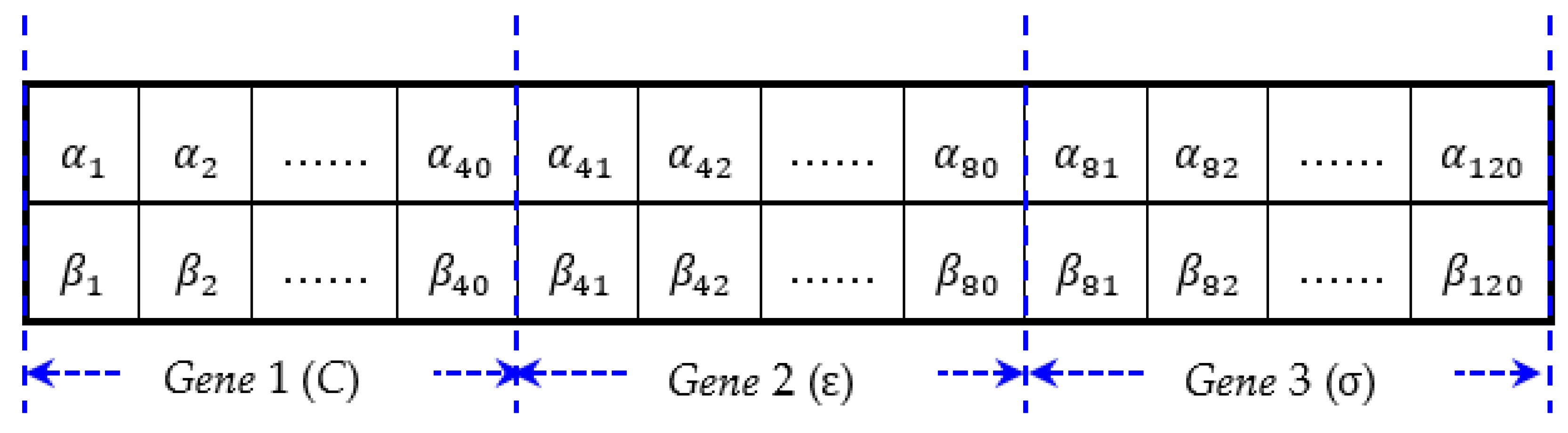
Step 1. Set up quantum chromosomes. In this paper, the quantum chromosome is composed of a string of m qubits (superposition of all possible states), as shown in Figure 2. These SVR’s three parameters, C, , and , are presented into the quantum qubit superposition format, i.e., each chromosome has three genes to represent it. Based on the authors’ practical trials and experience, choosing a gene with 40 bits could produce more satisfactory results, thus, a chromosome in total contains 120 qubits (i.e., m = 120). A gene that contains more qubits would be associated with better partitioning around the space.
Step 2. Initialize population. The population of the quantum chromosome is initialized by setting all the amplitudes of qubits as [30], i.e., all superposition states has equal probability in the initial population.
Step 3. Evaluate fitness (forecasting errors). Evaluate the objective fitness (forecasting errors) by using the values of each quantum chromosome. The mean absolute percentage error (MAPE), illustrated in Equation (18), is employed to measure the forecasting errors:
where N is the total number of forecasting results; is the actual value at each forecasting point i; is the forecasted value at each forecasting point i.
Step 4. Selection. In each generation, an elitist selection mechanism is used to select the best chromosome (with smallest MAPE value), i.e., the competition strategy is applied and as mentioned the best chromosome with the smallest MAPE value is recorded as the elitist and is reproduced as the initial chromosome for the next generation.
Step 5. Quantum crossover. To keep the population diversity, a quantum crossover operation is employed. Based on predefined crossover probability, Pcr (set as 0.9 [26]), the single-point-crossover principle is applied to randomly select two chromosomes to conduct crossover operation at any random position. For each generation, a new chromosomes pool would be generated after the quantum crossover operation is finished. Figure 3 illustrates the processed results of the quantum crossover operation.
Step 6. Quantum mutation. This is a useful approach to ensure population diversity. In this operation, each selected position of the participated quantum chromosome would be mutated with other real numbers according to the designate mutation probability, Pm (set as 0.1 [26]). Figure 4 shows an example of the quantum mutation operation.
Step 7. Quantum rotation gate. This operation modifies the oscillation ranges of individuals to improve the performance by changing the state of each qubit. It is performed by using a quantum rotation gate (as shown in Equation (16)), in which the rotation angle is a function of the oscillation amplitudes (,), and the value of the individual qubit located at the position i would also be modified accordingly [33]. The rotation angle is updated by Equation (19):
where is the current forecasting error; is the average value of all previous forecasting errors. Based on quantum genetic algorithm performance, a general criterion to set values between 0.1π and 0.005π [31].
Step 8. Premature convergence test. Compute the mean square error (MSE), given by Equation (20), to test the level of premature convergence [34], and set up the criterion value, δ:
where is given by Equation (21):
If the value of the calculated MSE is less than δ, it implies premature convergence occurs. Hence, the chaotic cat function (Equation (17)) is employed to escape the local optimum, i.e., finding out new optimum, and set the new optimum as the best solution.
Step 9. Stop criteria. If the number of generations is greater than a given scale, then, the best solution could be the presented quantum chromosomes; otherwise, go back to Step 3 and continue searching the next generation.
3. Experimental Examples
3.1. Data Sets of Experimental Examples
To compare the performances from the hybrid quantum-behaved evolutionary algorithms with an SVR model, this paper employs the same experimental examples used in Huang [27] and Lee and Lin [28]. These three experimental examples are: (1) the regional electricity load data in Taiwan from a published paper [23]; (2) the annual electricity load data in Taiwan from a published paper [23]; and (3) the electricity load data per hour from the 2014 Global Energy Forecasting Competition [35]. The data setting details for each examples are summarized in the following. The data characteristics of these three examples are summarized in Table 1.
3.1.1. Regional Electricity Load Data in Taiwan: Example 1
For Example 1, there are in total 20 years of regional electricity load values (from 1981 to 2000) for four regions in Taiwan. Based on the same forecasting performance comparison conditions, the modeling sub-data set division is the same as in a previous paper [23]. Thus, three subsets are obtained: a training subset (12 years of load data in total, from 1981 to 1992), a validation subset (a total of 4 years of data, from 1993 to 1996), and a testing subset (a total of 4 years of data, from 1997 to 2000). The well-known window-rolling procedure is employed during the whole process including the electricity load forecasts produced. For details of the window-rolling forecasting procedure readers should refer to Hong [23] and Lee and Lin [28]. Three parameters are determined by CQGA, while the validation error is also calculated. The most suitable parameters are finalized only when the smallest validation errors occur. Finally, the four-step (year) load forecasting for each region in Taiwan is implemented by the proposed SVRCQGA model.
3.1.2. Annual Electricity Load Data in Taiwan: Example 2
For Example 2, there are in total 59 annual electricity load values (from 1945 to 2003). Similarly, to make sure the same forecasting performance comparison conditions are used, the modeling sub-dataset division is the same as in a previous paper [23], i.e., a training subset (40 years of data, from 1945 to 1984), a validation subset (10 years of data, from 1985 to 1994), and a testing subset (9 years of data, from 1995 to 2003). The modeling processing details are almost as the same as in Example 1: the window-rolling procedure is applied, then, three parameters are also selected by CQGA. The most suitable parameters are finalized only based on the smallest validation errors. Eventually, the one-step (year) load forecasting in Taiwan is implemented using the proposed model.
3.1.3. 2014 Global Energy Forecasting Competition (GEFCOM 2014) Electricity Load Data: Example 3
For Example 3, there are a total of 744 h of electricity load data (from 00:00 1 December 2011 to 00:00 1 January 2012). Similarly, to be based on the same forecasting performance comparison conditions, the modeling sub-data set division is the same as in a previous paper [27,28]. Thus, we have a training subset (552 h of load data, from 01:00 1 December 2011 to 00:00 24 December 2011), a validation subset (96 h of load data, from 01:00 24 December 2011 to 00:00 28 December 2011), and a testing subset (96 h of load data, from 01:00 28 December 2011 to 00:00 1 January 2012). The modeling processing details are almost as the same as in the two previous examples: a window-rolling procedure is still used, and the most suitable three parameters must be finalized based only on the smallest validation errors. Finally, the one-step (hour) load forecasting results are obtained using the proposed model.
3.2. Parameters Setting & Forecasting Results and Analysis
3.2.1. Setting the CQGA Parameters
The parameters of CQGA for the three experimental examples are set practically: the population scale (Pscale) is set to be 200; the generations of the population (qmax) are no larger than 500; the qubit string length of a quantum chromosome (m) is set as 120; the probabilities of quantum crossover (Pcr) and quantum mutation (Pm) are set as 0.5 and 0.1 [26], respectively. Some controlled parameters during the modeling procedure are set as follows: the maximal iteration for each example is all set as 10,000 in each generation; , in all examples, in Example 1, in Examples 2 and 3; δ is fixed as 0.001.
3.2.2. Forecasting Accuracy Indexes
To comprehensively compare the forecasting accuracy for each models, the mean absolute percentage error (MAPE; as shown in Equation (18)), the root mean squared error (RMSE; as shown in Equation (22)), and the mean absolute error (MAE; as shown in Equation (23)) are employed:
where N is the total number of forecasting results; is the actual value at each forecasting point i; is the forecasted value at each forecasting point i.
3.2.3. Forecasting Performance Superiority Tests
To ensure the forecasting superiority of the proposed model is statistically significant, it is necessary to conduct some statistical tests to verify the significance of the proposed model. Based on Diebold and Mariano’s [36] and Derrac et al.’s [37] suggestions, two tests are conducted in this paper, they are Wilcoxon signed-rank test [38] and Friedman test [39].
(A) Wilcoxon Signed-rank Test
The Wilcoxon signed-rank test is used to detect the significance of a difference in the central tendency of two data series when the size of the two data series is equal. The statistic W is represented as Equation (24):
where:
where N is the total number of forecasting results.
(B) Friedman test
The Friedman test is used to measure the ANOVA in nonparametric statistical procedures; thus, it is a multiple comparisons test that aims to detect significant differences between the behaviors of two or more algorithms. The statistic F is represented as Equation (30):
where N is the total number of forecasting results; k is the number of compared models; Rj is the average rank sum obtained in each forecasting value for each algorithm as shown in Equation (31):
where is the rank sum from 1 (the smallest forecasting error) to k (the worst forecasting error) for ith forecasting result, for jth compared model.
The null hypothesis for Friedman’s test is that equality of forecasting errors among compared models. The alternative hypothesis is defined as the negation of the null hypothesis.
3.2.4. Results and Analysis: Example 1
For Example 1, SVR’s three parameter values determine the most suitable model for each region, which are computed by the QGA algorithm and CQGA algorithm, respectively, and with the smallest testing error (MAPE value). These determined parameters for each region are illustrated in Table 2.
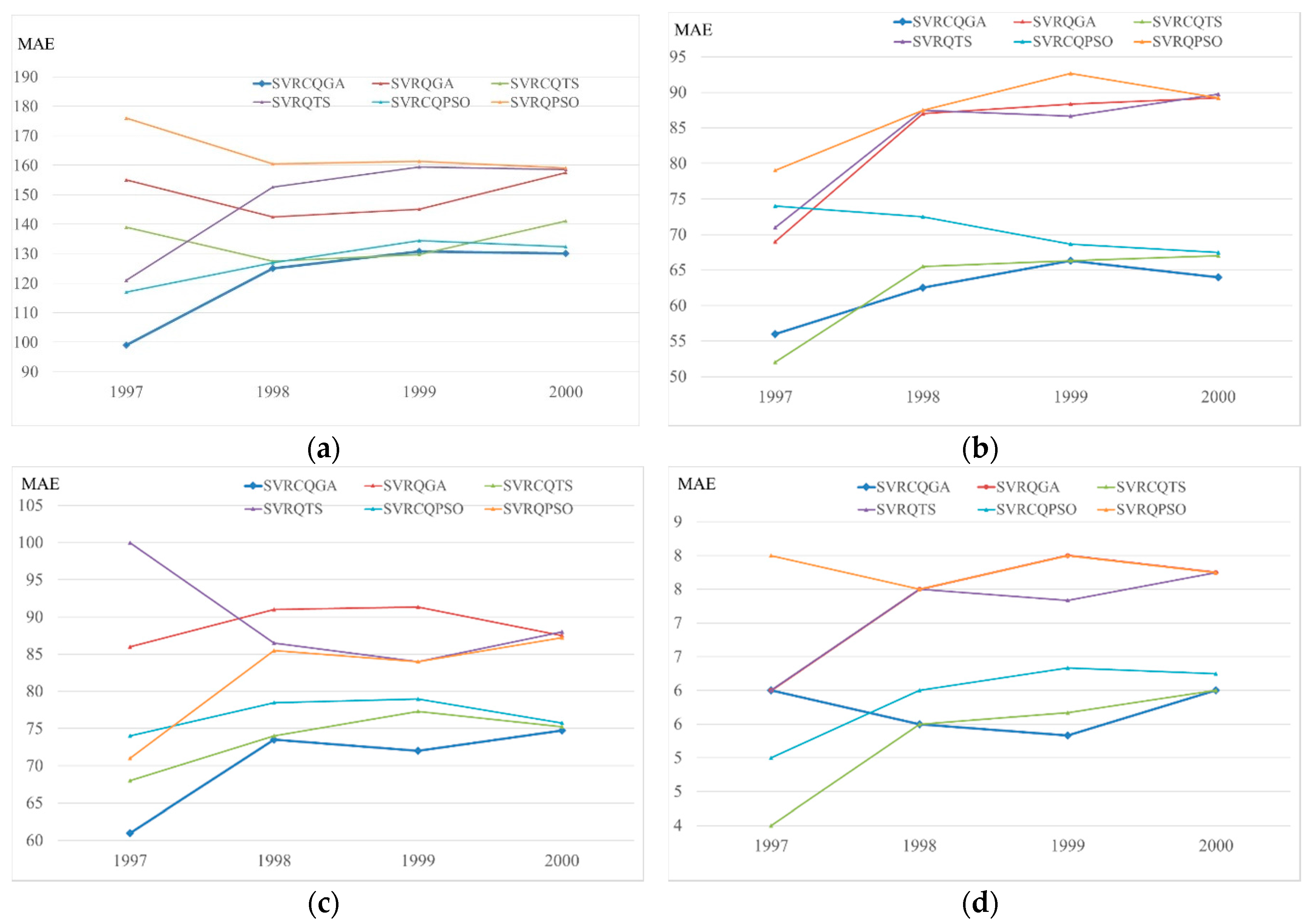
For forecasting results comparison details, Table 3 demonstrates the forecasting accuracy indexes of the proposed SVRCQGA and other competitive models [27,28] for each region. Figure 5 illustrates the cumulative differences of MAE for each competitive models in four regions. The competitive models include SVRCQPSO (hybrid SVR with chaotic quantum PSO) [27], SVRQPSO (hybrid SVR with quantum PSO) [27], SVRCQTS (hybrid SVR with chaotic quantum tabu search) [28], and SVRQTS (hybrid SVR with quantum tabu search) [28] models.
From Table 3 and Figure 5, it is obvious from the comparison that the proposed SVRCQGA model outperforms the other quantum-SVR-based models. Thus, it once again demonstrates the superiority of an SVR model in that it could obtain a more satisfactory forecasting performance by hybridizing quantum computing mechanics with a genetic algorithm. In the same time, the super capability of the cat mapping function in looking for a closer solution to the theoretical global optimum while suffering from premature convergence is noted. The QGA almost has done its best to look for the best solutions for each region, however, these solutions are still unsatisfactory by comparison with the performances of other alternatives. These solutions could be improved by employing a chaotic mapping function (this paper uses the cat mapping function), i.e., the CQGA, to achieve satisfactory solutions.
Then, two forecasting performance superiority tests are conducted. Table 4 shows the test results under a one-tail-test at α = 0.05 significance level, which point out that the proposed model achieves significantly better performance, except versus the SVRCQTS model.
3.2.5. Results and Analysis: Example 2
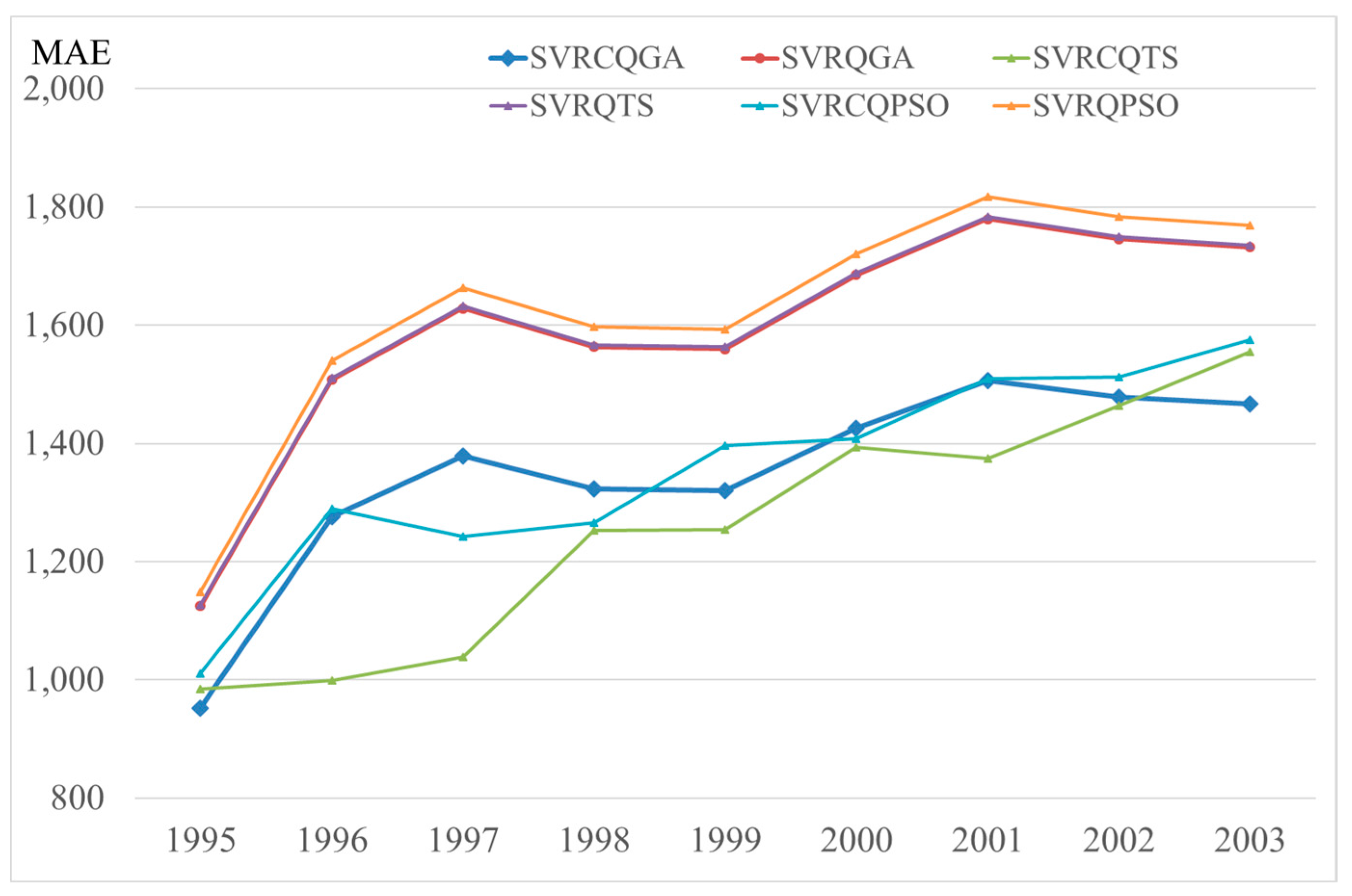
For Example 2, similarly, with the smallest MAPE values in the testing set, the SVR’s parameters are determined by the QGA algorithm and CQGA algorithm, respectively. These most suitable parameter values for the annual electricity load data are listed in Table 5. To benchmark the results with other research approaches, Table 5 also provides the forecasting index values from other competitive models [27,28].
The forecasting accuracy indexes values, MAPE and RMSE, are shown in Table 6. Figure 6 illustrates the cumulative differences of MAE for each competitive model. The competitive models also include the SVRCQPSO [27], SVRQPSO [27], SVRCQTS [28], and SVRQTS [28] models. Similarly, the proposed model receives an outstanding performance among other competitive models. The contributions of the quantum computing concepts and the chaotic cat mapping capability are again excellent. It is obviously that the CQGA algorithm excels at finding another better solution.
In Example 2, similarly, a Wilcoxon signed-rank test and Friedman test are also conducted to test the significance of the proposed model against the other competitive models. Both tests results are illustrated in Table 7, and demonstrate clearly that the proposed model significantly outperforms the other quantum-behaved algorithms with SVR-based forecasting models.
3.2.6. Results and Analysis: Example 3
For Example 3, based on the similar modeling processes, the SVR’s three parameters are eventually selected by the QGA algorithm and CQGA algorithm, respectively. The details of the most suitable parameters of all employed compared models for GEFCOM 2014 data set are shown in Table 8. Because references [27,28] also use GEFCOM 2014 load data set for analysis, therefore, those models shown in [27,28] are also compared with the proposed models.
To achieve a meaningful comparison, the authors only selected three quantum- and SVR-based forecasting models, i.e., the SVRCQGA, SVRCQTS, and SVRCQPSO models, to compare with each other. Table 9 provides the forecasting accuracy indexes of the proposed SVRCQGA and other competitive models [27,28], and clearly illustrates that the proposed SVRCQGA model achieves results closer to the actual load values than the SVRCQTS and SVRCQPSO models.
4. Conclusions
This paper proposes a novel electricity load forecasting model created by hybridizing a quantum-behaved algorithm with an SVR-based model. The results have completely shown that the proposed CQGA has superiority to address the embedded drawbacks of the original GA and quantum GA algorithms that suffer from getting trapped into local optima. This paper uses quantum computing mechanics to enrich the diversity of the population during the GA modeling processes, which eventually improves the forecasting accuracy level. The cat function is employed to avoid premature convergence while the QGA algorithm is processing. This paper provides support to continue the exploration of integrating quantum computing concepts and chaotic mapping techniques to enrich the search space with the limitations from conventional Newtonian dynamics, and a more effective approach to solve the trapping in local optima problem.
Author Contributions
Cheng-Wen Lee and Bing-Yi Lin conceived and designed the experiments; Bing-Yi Lin performed the experiments, analyzed the data and wrote the paper. Bing-Yi Lin is under Cheng-Wen Lee’s supervision.
Conflicts of Interest
The author declares no conflict of interest.
References
- Xiao, L.; Shao, W.; Liang, T.; Wang, C. A combined model based on multiple seasonal patterns and modified firefly algorithm for electrical load forecasting. Appl. Energy 2016, 167, 135–153. [Google Scholar] [CrossRef]
- Fan, S.; Chen, L. Short-term load forecasting based on an adaptive hybrid method. IEEE Trans. Power Syst. 2006, 21, 392–401. [Google Scholar] [CrossRef]
- Cincotti, S.; Gallo, G.; Ponta, L.; Raberto, M. Modelling and forecasting of electricity spot-prices: Computational intelligence vs. classical econometrics. AI Commun. 2014, 27, 301–314. [Google Scholar]
- Amjady, N.; Keynia, F. Day ahead price forecasting of electricity markets by a mixed data model and hybrid forecast method. Int. J. Electr. Power Energy Syst. 2008, 30, 533–546. [Google Scholar] [CrossRef]
- Weron, R. Electricity price forecasting: A review of the state-of-the-art with a look into the future. Int. J. Forecast. 2014, 30, 1030–1081. [Google Scholar] [CrossRef]
- Fan, G.; Peng, L.-L.; Hong, W.-C.; Sun, F. Electric load forecasting by the SVR model with differential empirical mode decomposition and auto regression. Neurocomputing 2016, 173, 958–970. [Google Scholar] [CrossRef]
- Hussain, A.; Rahman, M.; Memon, J.A. Forecasting electricity consumption in Pakistan: The way forward. Energy Policy 2016, 90, 73–80. [Google Scholar] [CrossRef]
- Vu, D.H.; Muttaqi, K.M.; Agalgaonkar, A.P. A variance inflation factor and backward elimination based Robust regression model for forecasting monthly electricity demand using climatic variables. Appl. Energy 2015, 140, 385–394. [Google Scholar] [CrossRef]
- Maçaira, P.M.; Souza, R.C.; Oliveira, F.L.C. Modelling and forecasting the residential electricity consumption in Brazil with pegels exponential smoothing techniques. Procedia Comput. Sci. 2015, 55, 328–335. [Google Scholar] [CrossRef]
- Al-Hamadi, H.M.; Soliman, S.A. Short-term electric load forecasting based on Kalman filtering algorithm with moving window weather and load model. Electr. Power Syst. Res. 2004, 68, 47–59. [Google Scholar] [CrossRef]
- Hippert, H.S.; Taylor, J.W. An evaluation of Bayesian techniques for controlling model complexity and selecting inputs in a neural network for short-term load forecasting. Neural Netw. 2010, 23, 386–395. [Google Scholar] [CrossRef] [PubMed]
- Kelo, S.; Dudul, S. A wavelet Elman neural network for short-term electrical load prediction under the influence of temperature. Int. J. Electr. Power Energy Syst. 2012, 43, 1063–1071. [Google Scholar] [CrossRef]
- Lahouar, A.; Slama, J.B.H. Day-ahead load forecast using random forest and expert input selection. Energy Convers. Manag. 2015, 103, 1040–1051. [Google Scholar] [CrossRef]
- Chaturvedi, D.K.; Sinha, A.P.; Malik, O.P. Short term load forecast using fuzzy logic and wavelet transform integrated generalized neural network. Int. J. Electr. Power Energy Syst. 2015, 67, 230–237. [Google Scholar] [CrossRef]
- Zhai, M.-Y. A new method for short-term load forecasting based on fractal interpretation and wavelet analysis. Int. J. Electr. Power Energy Syst. 2015, 69, 241–245. [Google Scholar] [CrossRef]
- Coelho, V.N.; Coelho, I.M.; Coelho, B.N.; Reis, A.J.R.; Enayatifar, R.; Souza, M.J.F.; Guimarães, F.G. A self-adaptive evolutionary fuzzy model for load forecasting problems on smart grid environment. Appl. Energy 2016, 169, 567–584. [Google Scholar] [CrossRef]
- Bahrami, S.; Hooshmand, R.-A.; Parastegari, M. Short term electric load forecasting by wavelet transform and grey model improved by PSO (particle swarm optimization) algorithm. Energy 2014, 72, 434–442. [Google Scholar] [CrossRef]
- Aras, S.; Kocakoç, İ.D. A new model selection strategy in time series forecasting with artificial neural networks: IHTS. Neurocomputing 2016, 174, 974–987. [Google Scholar] [CrossRef]
- Kendal, S.L.; Creen, M. An Introduction to Knowledge Engineering; Springer: London, UK, 2007. [Google Scholar]
- Cherroun, L.; Hadroug, N.; Boumehraz, M. Hybrid approach based on ANFIS models for intelligent fault diagnosis in industrial actuator. J. Control Electr. Eng. 2013, 3, 17–22. [Google Scholar]
- Hahn, H.; Meyer-Nieberg, S.; Pickl, S. Electric load forecasting methods: Tools for decision making. Eur. J. Oper. Res. 2009, 199, 902–907. [Google Scholar] [CrossRef]
- Drucker, H.; Burges, C.C.J.; Kaufman, L.; Smola, A.; Vapnik, V. Support vector regression machines. Adv. Neural Inf. Process. Syst. 1997, 9, 155–161. [Google Scholar]
- Hong, W.C. Chaotic particle swarm optimization algorithm in a support vector regression electric load forecasting model. Energy Convers. Manag. 2009, 50, 105–117. [Google Scholar] [CrossRef]
- Hong, W.C. Electric load forecasting by seasonal recurrent SVR (support vector regression) with chaotic artificial bee colony algorithm. Energy 2011, 36, 5568–5578. [Google Scholar] [CrossRef]
- Bhunia, C.T. Quantum computing & information technology: A tutorial. IETE J. Educ. 2006, 47, 79–90. [Google Scholar]
- Dey, S.; Bhattacharyya, S.; Maulik, U. Quantum inspired genetic algorithm and particle swarm optimization using chaotic map model based interference for gray level image thresholding. Swarm Evol. Comput. 2014, 15, 38–57. [Google Scholar] [CrossRef]
- Huang, M.-L. Hybridization of chaotic quantum particle swarm optimization with SVR in electric demand forecasting. Energies 2016, 9, 426. [Google Scholar] [CrossRef]
- Lee, C.-W.; Lin, B.-Y. Application of hybrid quantum tabu search with support vector regression (SVR) for load forecasting. Energies 2016, 9, 873. [Google Scholar] [CrossRef]
- Shor, P.W. Algorithms for quantum computation: Discrete logarithms and factoring. In Proceedings of the 35th Annual Symposium on Foundations of Computer Science, Santa Fe, NM, USA, 20–22 November 1994; pp. 124–134. [Google Scholar]
- Han, K.-H. Quantum-inspired evolutionary algorithms with a new termination criterion, Hε gate, and two-phase scheme. IEEE Trans. Evol. Comput. 2004, 8, 156–169. [Google Scholar]
- Lahoz-Beltra, R. Quantum genetic algorithms for computer scientists. Computers 2016, 5, 24. [Google Scholar] [CrossRef]
- Chen, G.; Mao, Y.; Chui, C.K. Asymmetric image encryption scheme based on 3D chaotic cat maps. Chaos Solitons Fract. 2004, 21, 749–761. [Google Scholar] [CrossRef]
- Hang, B.; Jiang, J.; Gao, Y.; Ma, Y. A Quantum Genetic Algorithm to Solve the Problem of Multivariate. In Information Computing and Applications, Proceedings of the Second International Conference ICICA 2011, Qinhuangdao, China, 28–31 October 2011; Liu, C., Chang, J., Yang, A., Eds.; Springer: Berlin/Heidelberg, Germany, 2011; pp. 308–314. [Google Scholar]
- Su, H. Chaos quantum-behaved particle swarm optimization based neural networks for short-term load forecasting. Procedia Eng. 2011, 15, 199–203. [Google Scholar] [CrossRef]
- 2014 Global Energy Forecasting Competition Site. Available online: http://www.drhongtao.com/gefcom/ (accessed on 9 November 2017).
- Diebold, F.X.; Mariano, R.S. Comparing predictive accuracy. J. Bus. Econ. Stat. 1995, 13, 134–144. [Google Scholar]
- Derrac, J.; García, S.; Molina, D.; Herrera, F. A practical tutorial on the use of nonparametric statistical tests as a methodology for comparing evolutionary and swarm intelligence algorithms. Swarm Evol. Comput. 2011, 1, 3–18. [Google Scholar] [CrossRef]
- Wilcoxon, F. Individual comparisons by ranking methods. Biom. Bull. 1945, 1, 80–83. [Google Scholar] [CrossRef]
- Friedman, M. A comparison of alternative tests of significance for the problem of m rankings. Ann. Math. Stat. 1940, 11, 86–92. [Google Scholar] [CrossRef]
Figure 1.
Quantum genetic algorithm flowchart.
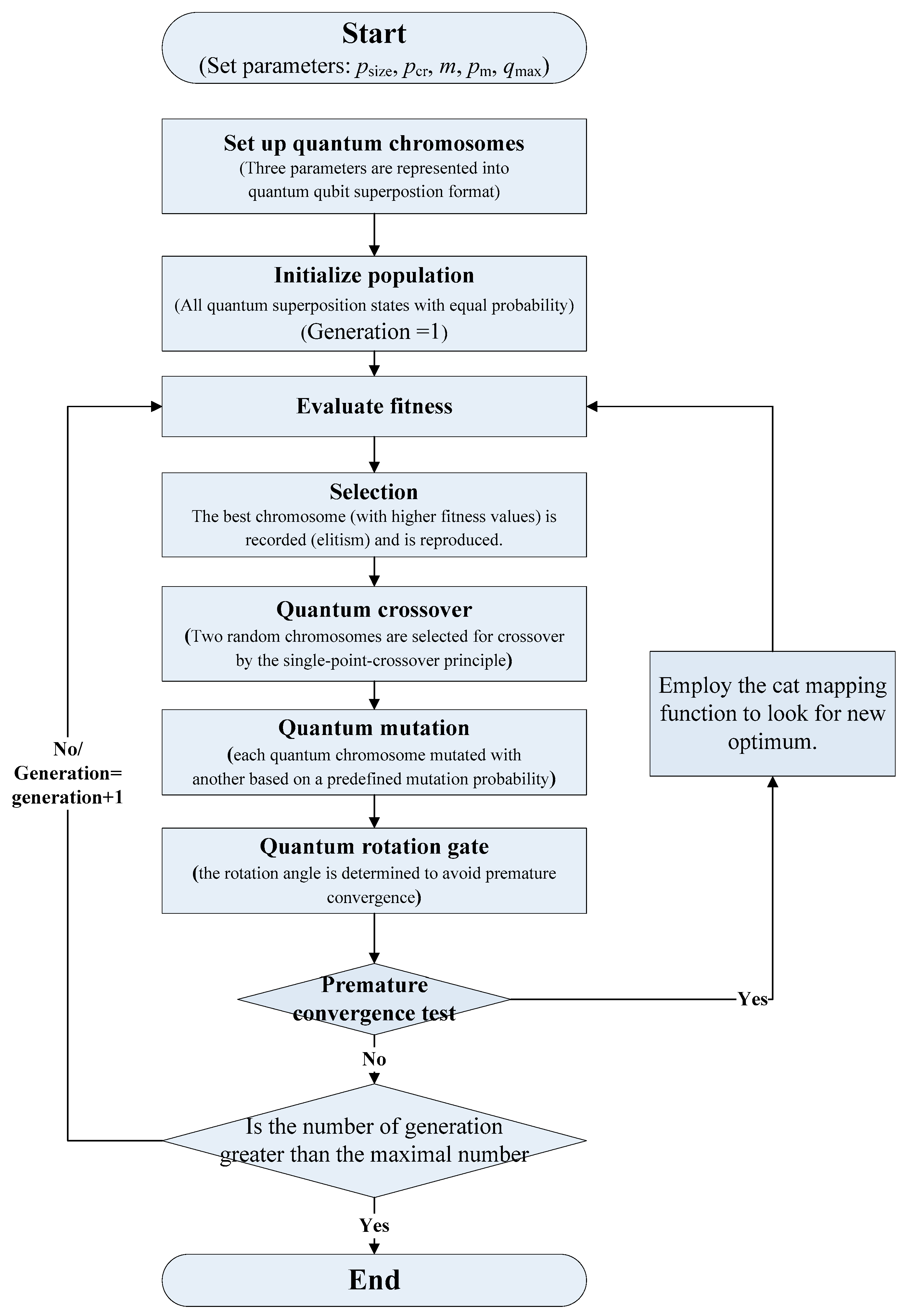
Figure 2.
Quantum chromosome structure for three parameters.

Figure 3.
Example of the chromosome form of the parameters for the quantum crossover operation.
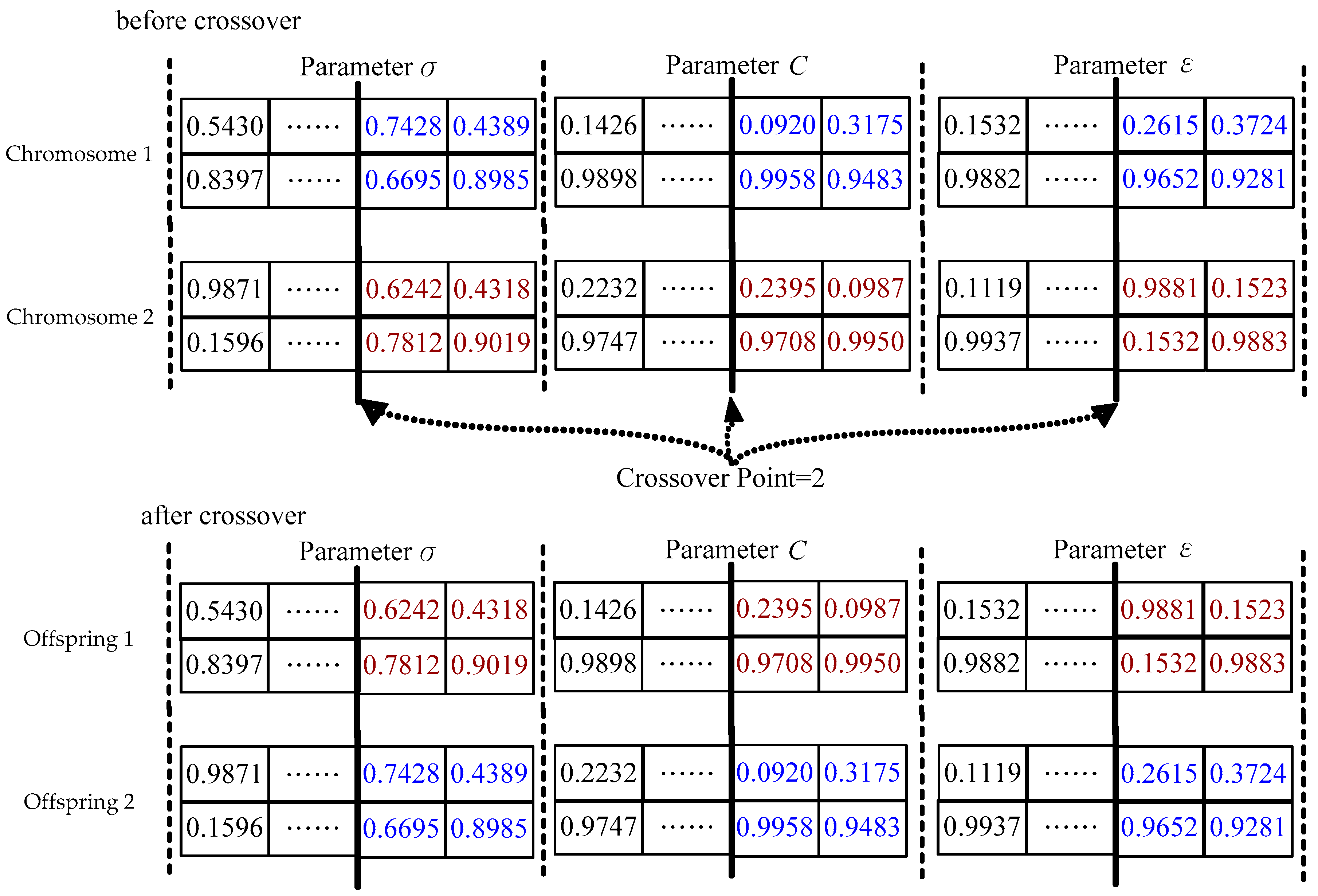
Figure 4.
Example of the chromosome form of the parameter for the quantum mutation operation.
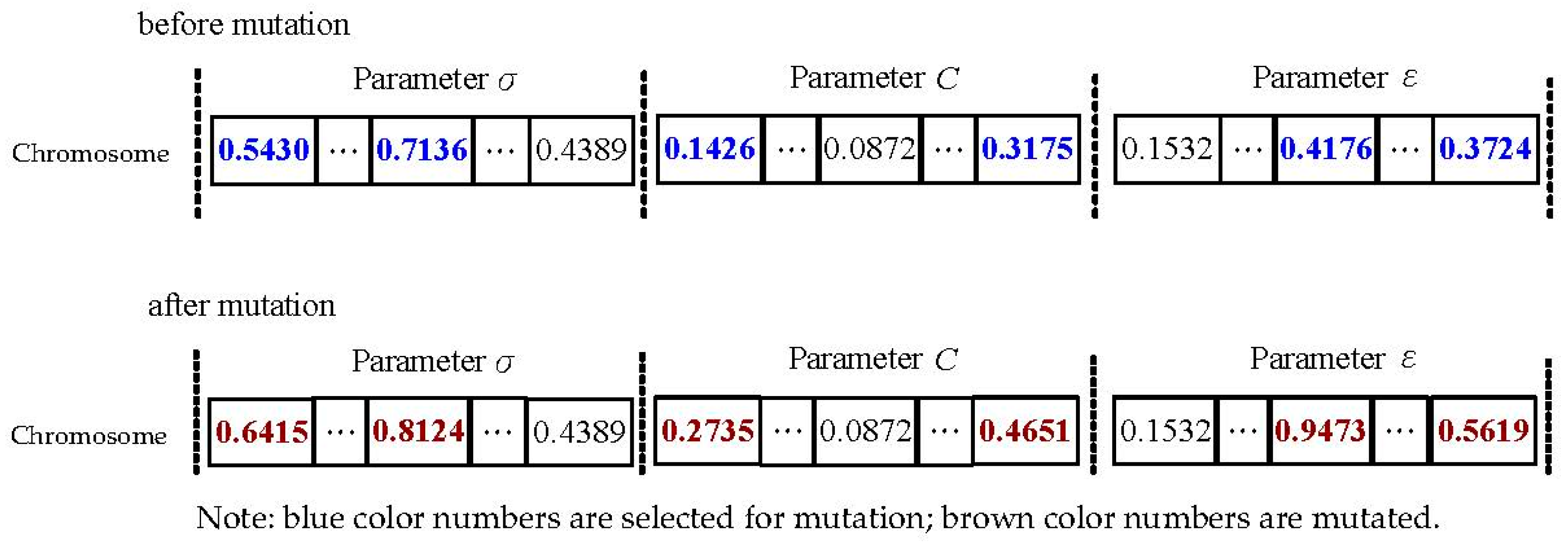
Figure 5.
The cumulative differences of MAE for each competitive models in four regions (Example 1). (a) Northern region; (b) Central Region; (c) Southern region; (d) Eastern region.
Figure 5.
The cumulative differences of MAE for each competitive models in four regions (Example 1). (a) Northern region; (b) Central Region; (c) Southern region; (d) Eastern region.

Figure 6.
The cumulative differences of MAE for each competitive model (Example 2).

Figure 7.
The cumulative differences of MAE for each competitive model (Example 3).


Table 1.
Data characteristics summary of three examples.
| Examples | Data Type | Data Length | Data Size | Data Characteristics |
|---|---|---|---|---|
| Example 1 | Regional and annual | From 1981 to 2000 | 4 regions and 20 years | Increment with fluctuation caused by some accidental event (921 earthquake) |
| Example 2 | Annual | From 1945 to 2003 | 59 years | Increment with the continuous economic development in Taiwan |
| Example 3 | Hourly | From 1 December 2011 to 1 January 2012 | 744 h | Cyclic fluctuation |
Table 2.
Determined parameters of SVRCQGA and SVRQGA models (Example 1).
| Regions | SVRCQGA Parameters | MAPE of Testing (%) | ||
| σ | C | ε | ||
| Northern | 4.0000 | 0.6500 | 1.0760 | |
| Central | 6.0000 | 0.3500 | 1.2130 | |
| Southern | 8.0000 | 0.4800 | 1.1650 | |
| Eastern | 12.0000 | 0.2800 | 1.5180 | |
| Regions | SVRQGA Parameters | MAPE of Testing (%) | ||
| σ | C | ε | ||
| Northern | 3.0000 | 0.3400 | 1.3150 | |
| Central | 10.0000 | 0.4800 | 1.6830 | |
| Southern | 6.0000 | 0.3500 | 1.3640 | |
| Eastern | 4.0000 | 0.6800 | 1.9680 | |
Table 3.
Forecasting indexes of SVRCQGA, SVRQGA, and other models (Example 1).
| Indexes | SVRCQGA | SVRQGA | SVRCQTS | SVRQTS | SVRCQPSO | SVRQPSO |
|---|---|---|---|---|---|---|
| Northern region | ||||||
| MAPE (%) | 1.0760 | 1.3150 | 1.0870 | 1.3260 | 1.1070 | 1.3370 |
| RMSE | 131.48 | 159.26 | 132.79 | 159.43 | 142.62 | 160.28 |
| MAE | 130.00 | 157.50 | 141.00 | 158.50 | 132.25 | 159.00 |
| Central region | ||||||
| MAPE (%) | 1.2130 | 1.6830 | 1.2650 | 1.6870 | 1.2840 | 1.6890 |
| RMSE | 64.46 | 90.18 | 67.69 | 90.67 | 67.70 | 89.87 |
| MAE | 64.00 | 89.25 | 67.00 | 89.75 | 67.50 | 89.25 |
| Southern region | ||||||
| MAPE (%) | 1.1650 | 1.3640 | 1.1720 | 1.3670 | 1.1840 | 1.3590 |
| RMSE | 75.44 | 87.82 | 75.57 | 88.84 | 76.03 | 88.05 |
| MAE | 74.75 | 87.50 | 75.25 | 88.00 | 75.75 | 87.25 |
| Eastern region | ||||||
| MAPE (%) | 1.5180 | 1.9680 | 1.5430 | 1.9720 | 1.5940 | 1.9830 |
| RMSE | 6.12 | 7.86 | 6.38 | 7.95 | 6.30 | 7.79 |
| MAE | 6.00 | 7.75 | 6.00 | 7.75 | 6.25 | 7.75 |
Table 4.
Wilcoxon signed-rank test and Friedman test (Example 1).
| Compared Models | Wilcoxon Signed-Rank Test α = 0.05; Wilcoxon W Statistic = 0 | Friedman Test α = 0.05 |
|---|---|---|
| Northern region | H0: e1 = e2 = e3 = e4 = e5 = e6 F = 12.46; p = 0.028 (reject H0) | |
| SVRCQGA vs. SVRQPSO | W = 0 * | |
| SVRCQGA vs. SVRCQPSO | W = 0 * | |
| SVRCQGA vs. SVRQTS | W = 0 * | |
| SVRCQGA vs. SVRCQTS | W = 1 | |
| SVRCQGA vs. SVRQGA | W = 0 * | |
| Central region | H0: e1 = e2 = e3 = e4 = e5 = e6 F = 13.43; p = 0.021 (reject H0) | |
| SVRCQGA vs. SVRQPSO | W = 0 * | |
| SVRCQGA vs. SVRCQPSO | W = 0 * | |
| SVRCQGA vs. SVRQTS | W = 0 * | |
| SVRCQGA vs. SVRCQTS | W = 1 | |
| SVRCQGA vs. SVRQGA | W = 0 * | |
| Southern region | H0: e1 = e2 = e3 = e4 = e5 = e6 F = 15.57; p = 0.013 (reject H0) | |
| SVRCQGA vs. SVRQPSO | W = 0 * | |
| SVRCQGA vs. SVRCQPSO | W = 0 * | |
| SVRCQGA vs. SVRQTS | W = 0 * | |
| SVRCQGA vs. SVRCQTS | W = 1 | |
| SVRCQGA vs. SVRQGA | W = 0 * | |
| Eastern region | H0: e1 = e2 = e3 = e4 = e5 = e6 F = 11.34; p = 0.035 (reject H0) | |
| SVRCQGA vs. SVRQPSO | W = 0 * | |
| SVRCQGA vs. SVRCQPSO | W = 0 * | |
| SVRCQGA vs. SVRQTS | W = 0 * | |
| SVRCQGA vs. SVRCQTS | W = 1 | |
| SVRCQGA vs. SVRQGA | W = 0 * |
* Denotes that the SVRCQGA model significantly outperforms other competitive models.
Table 5.
Determined parameters of SVRCQGA and SVRQGA models (Example 2).
| Optimization Algorithms | Parameters | MAPE of Testing (%) | ||
|---|---|---|---|---|
| σ | C | ε | ||
| QPSO algorithm [27] | 12.0000 | 0.380 | 1.3460 | |
| CQPSO algorithm [27] | 10.0000 | 0.560 | 1.1850 | |
| QTS algorithm [28] | 5.0000 | 0.630 | 1.3210 | |
| CQTS algorithm [28] | 6.0000 | 0.340 | 1.1540 | |
| QGA algorithm | 9.0000 | 0.480 | 1.3180 | |
| CQGA algorithm | 12.0000 | 0.650 | 1.1160 | |
Table 6.
Forecasting indexes of SVRCQGA, SVRQGA, and other models (Example 2).
| Years | SVRCQGA | SVRQGA | SVRCQTS | SVRQTS | SVRCQPSO | SVRQPSO |
|---|---|---|---|---|---|---|
| MAPE (%) | 1.1160 | 1.3180 | 1.1540 | 1.3210 | 1.1850 | 1.3460 |
| RMSE | 1502.66 | 1774.62 | 1631.48 | 1778.74 | 1618.34 | 1812.51 |
| MAE | 1466.33 | 1731.78 | 1554.89 | 1735.78 | 1575.67 | 1768.78 |
Table 7.
Wilcoxon signed-rank test and Friedman test (Example 2).
| Compared Models | Wilcoxon Signed-Rank Test α = 0.05; Wilcoxon W Statistic = 8 | Friedman Test α = 0.05 |
|---|---|---|
| SVRCQGA vs. SVRQPSO | W = 4 * | H0: e1 = e2 = e3 = e4 = e5 = e6 F = 13.35; p = 0.022 (reject H0) |
| SVRCQGA vs. SVRCQPSO | W = 2 * | |
| SVRCQGA vs. SVRQTS | W = 4 * | |
| SVRCQGA vs. SVRCQTS | W = 4 * | |
| SVRCQGA vs. SVRQGA | W = 4 * |
* Denotes that the SVRCQGA model significantly outperforms other competitive models.
Table 8.
Determined parameters of SVRCQGA, SVRQGA, and other models (Example 3).
| Optimization Algorithms | Parameters | MAPE of Testing (%) | ||
|---|---|---|---|---|
| σ | C | ε | ||
| QPSO algorithm [27] | 9.000 | 42.000 | 0.1800 | 1.9600 |
| CQPSO algorithm [27] | 19.000 | 35.000 | 0.8200 | 1.2900 |
| QTS algorithm [28] | 25.000 | 67.000 | 0.0900 | 1.8900 |
| CQTS algorithm [28] | 12.000 | 26.000 | 0.3200 | 1.3200 |
| QGA algorithm | 5.000 | 79.000 | 0.3800 | 1.7500 |
| CQGA algorithm | 6.000 | 54.000 | 0.6200 | 1.1700 |
Table 9.
Forecasting indexes of SVRCQGA, SVRQGA, and other models (Example 3).
| Indexes | SVRCQGA | SVRQGA | SVRCQTS | SVRQTS | SVRCQPSO | SVRQPSO |
|---|---|---|---|---|---|---|
| MAPE (%) | 1.1700 | 1.7500 | 1.3200 | 1.8900 | 1.2900 | 1.9600 |
| RMSE | 1.4927 | 1.6584 | 1.9909 | 2.8507 | 1.9257 | 2.9358 |
| MAE | 1.4522 | 1.6174 | 1.8993 | 2.7181 | 1.8474 | 2.8090 |
Table 10.
Wilcoxon signed-rank test and Friedman test (Example 3).
| Compared Models | Wilcoxon Signed-Rank Test | Friedman Test | |
|---|---|---|---|
| α = 0.05; Wilcoxon W Statistic = 2328 | p-Value | α = 0.05 | |
| SVRCQGA vs. SVRQPSO | W = 1278.0 * | 0.00012 | H0: e1 = e2 = e3 = e4 = e5 = e6 F = 71.266; p = 0.000 (reject H0) |
| SVRCQGA vs. SVRCQPSO | W = 1152.5 * | 0.00000 | |
| SVRCQGA vs. SVRQTS | W = 1256.0 * | 0.00000 | |
| SVRCQGA vs. SVRCQTS | W = 1263.0 * | 0.00010 | |
| SVRCQGA vs. SVRQGA | W = 2134.5 * | 0.00720 | |
* Denotes that the SVRCQGA model significantly outperforms the other competitive models.
© 2017 by the authors. Licensee MDPI, Basel, Switzerland. This article is an open access article distributed under the terms and conditions of the Creative Commons Attribution (CC BY) license (http://creativecommons.org/licenses/by/4.0/).
Share and Cite
MDPI and ACS Style
Lee, C.-W.; Lin, B.-Y. Applications of the Chaotic Quantum Genetic Algorithm with Support Vector Regression in Load Forecasting. Energies 2017, 10, 1832. https://doi.org/10.3390/en10111832
AMA Style
Lee C-W, Lin B-Y. Applications of the Chaotic Quantum Genetic Algorithm with Support Vector Regression in Load Forecasting. Energies. 2017; 10(11):1832. https://doi.org/10.3390/en10111832
Chicago/Turabian StyleLee, Cheng-Wen, and Bing-Yi Lin. 2017. "Applications of the Chaotic Quantum Genetic Algorithm with Support Vector Regression in Load Forecasting" Energies 10, no. 11: 1832. https://doi.org/10.3390/en10111832
Note that from the first issue of 2016, this journal uses article numbers instead of page numbers. See further details here.