Numerical Investigation of the Tip Vortex of a Straight-Bladed Vertical Axis Wind Turbine with Double-Blades

1
College of Mechanical Engineering, Inner Mongolia University of Technology, Hohhot 010051, China
2
Graduate School of Bioresources, Mie University, 1577 Kurimamachiya-cho, Tsu, Mie 514-8507, Japan
3
Division of Mechanical Engineering, Mie University, 1577 Kurimamachiya-cho, Tsu, Mie 514-8507, Japan
*
Authors to whom correspondence should be addressed.
Energies 2017, 10(11), 1721; https://doi.org/10.3390/en10111721
Submission received: 5 September 2017
/
Revised: 23 October 2017
/
Accepted: 23 October 2017
/
Published: 27 October 2017
(This article belongs to the Collection Wind Turbines)
Abstract
:Wind velocity distribution and the vortex around the wind turbine present a significant challenge in the development of straight-bladed vertical axis wind turbines (VAWTs). This paper is intended to investigate influence of tip vortex on wind turbine wake by Computational Fluid Dynamics (CFD) simulations. In this study, the number of blades is two and the airfoil is a NACA0021 with chord length of c = 0.265 m. To capture the tip vortex characteristics, the velocity fields are investigated by the Q-criterion iso-surface (Q = 100) with shear-stress transport (SST) k-ω turbulence model at different tip speed ratios (TSRs). Then, mean velocity, velocity deficit and torque coefficient acting on the blade in the different spanwise positions are compared. The wind velocities obtained by CFD simulations are also compared with the experimental data from wind tunnel experiments. As a result, we can state that the wind velocity curves calculated by CFD simulations are consistent with Laser Doppler Velocity (LDV) measurements. The distribution of the vortex structure along the spanwise direction is more complex at a lower TSR and the tip vortex has a longer dissipation distance at a high TSR. In addition, the mean wind velocity shows a large value near the blade tip and a small value near the blade due to the vortex effect.
1. Introduction
Horizontal axis wind turbines (HAWTs) have developed rapidly since the aggravation of the fossil energy crisis. However, they are mainly installed in areas away from high electricity demand, such as plains, mountains, etc., resulting in high infrastructure costs and high transmission losses [1]. Recently, a small type of vertical axis wind turbine (VAWT) has attracted the attention of many researchers due to its power coefficient being less affected by the high turbulence intensity in the urban environment. Meanwhile, its noise is very low because of the low tip speed ratio [2,3,4,5]. However, the resultant velocity to blade and the angle of attack can change periodically with the azimuth angle θ, and the blade will generate dynamic stalls and tip vortexes. This phenomenon can generate a blade vortex and cause a strong or sudden flow separation on the suction surface. This vortex travels along with the blade surface as it grows, and finally separates from the airfoil at the leading edge [6,7]. Then the tip vortex shedding from the upstream blade can affect the aerodynamic performance of the downstream blade. Meanwhile, the flow field around the wind turbine has a rather complex vortex structure and wind velocity distribution [8,9,10]. Therefore, any study on power performance of VAWTs needs to take into account the evolution of their flow field, especially the tip vortex effect.
Over the past few years, the study on the flow field of VAWT has achieved some results through CFD simulations, wind tunnel experiments and field tests. In 2012, Hofemann et al. [11] studied the detailed development of field flows and vortexes around the rotor with the Particle Image Velocimetry (PIV) technology. The results showed that the previous shedding vortex could affect the development of a new vortex and the vortex intensity increased with the increase of the angle of attack. Sun et al. [12] in 2014 and Li et al. [13] in 2017 investigated the wind velocity distribution of flow fields around the VAWT at different TSRs by experimental measurements. In their studies, a wide range of low wind velocities was found from the internal region to the near-wake of the wind turbine. In addition, with the increase of TSR, the low wind velocity regions had an expansion trend in the wind turbine wake. However, they only studied the effect of TSR on the flow field of VAWTs, rather than the aerodynamic performance. In order to investigate the effect of TSR on the aerodynamic characteristics of VAWTs, Chen and Lian [14] studied the effects of solidity and TSR on the torque and power coefficients of wind turbines with CFD simulations on the basis of a Navier-Stokes solver. The results demonstrated that the maximum power coefficient of the rotor increased and maximum torque coefficient decreased with the increase of solidity. Although the characteristics of VAWTs were well investigated, the resultant flow velocity and the angle of attack were calculated with the mainstream wind velocity. In 2016 Li et al. [15] calculated the resultant flow velocity and angle of attack with the local wind velocity at three different TSRs by measurements with a Laser Doppler Velocity (LDV) system. They found that the resultant wind velocity increased and the maximum value of the angle of attack decreased with the increase of TSR. After that, to study the turbulence intensity effect on the wake field in natural wind, Li et al. [16] in 2016 further explored the velocity distribution of flow fields around the rotors by field tests. From their study, it was found that the wind velocity in the field test had a quicker recovery than that in the wind tunnel. Furthermore, the wind velocity was further reduced with the increase of TSR. However, the PIV and LDV technology in the wind tunnel are only the measurements of defined areas and points. CFD simulation can simulate the whole flow field of a VAWT. In 2016, Posa et al. [17] measured the wake structure of a straight-bladed VAWT with double-blades at two different TSRs. They compared the wake distribution by using PIV measurements and Large Eddy Simulation (LES) in a three-dimensional (3D) condition. According to their study, a strong dynamic stall was found in both the upstream region and downstream region at a low TSR. Meanwhile, the dynamic stall of the blade in the upstream region was stronger than that in the downstream region. Regrettably, more details about the tip vortex were not examined.
Studies on the dynamic stall of VAWT have also achieved some results through CFD simulations and wind tunnel experiments. In 1986 Vittencoq [18] indicated the evolution of the dynamic stall of blade surface in detail at Reynolds number of 3.8 × 10⁴ and different TSRs with 2D CFD simulations. In this study, in the case of stall, the vortex was formed on the trailing edge of blade, advanced along the upper surface of blade toward the leading edge, and began to fall off as it moved with 1/3 of the tangential velocity of blade. In 2009 Ferreira et al. [19] researched the dynamic stall characteristics on the blade in the case of 3D by using PIV measurement at the azimuth angle of 0° < θ < 360°. In this study, the evolution of the flow field was not only affected by the variations of the angle of attack, but also by the formation, roll-up, release and interaction of the shedding vortex. In order to investigate the subtle changes of dynamic stall, Qin et al. [20] in 2011 computed the evolution of the dynamic stall of rotor in the condition of low-to-moderate Reynolds number, based on the unsteady Reynolds-averaged Navier-Stokes (RANS) equations. In this study, they found that the model not only saved computation time, but also improved the precision of the CFD simulations. In addition, in 2014 Lanzafame et al. [21], in 2015 Buchner et al. [22] and in 2016 Dunne [23] also reached similar conclusions.
In 2014, Sun et al. [24] analyzed the influence of the interaction between shedding vortices on the flow field around the rotor at different TSRs. They described that the shedding vortex of the blade had an important impact on the aerodynamics and the flow field around the wind turbine in a low TSR. This influence decreased with the increase of the chord length of blade. However, Sun et al. didn’t investigate the subtle structure of the vortex. In 2016, Chatelain et al. [25] put forward a new method based on the vorticity-velocity formulation of the Navier-Stokes equations and the vortex particle grid. This new method was effective to simulate the vortex structure of the wake of VAWT. They not only found that the data obtained from the new method was very similar to the experimental data obtained by PIV, but also showed the development of the complex wake in detail. In 2017 Thé and Yu [26] also got the similar results by a free vortex model. Moreover, Li et al. [27] studied the effect of solidity and rotor aspect ratio on the circulation amount and power coefficient using the panel method in the condition of three-dimensional model. In their study, the rotor aspect ratio was only affected by the airflow near the blade tip. In addition, in 2016 Li et al. [28,29] discussed the influence of the shedding vortex of blade on the flow field around blade by using LDV system. The results suggested that the wind velocity in the surface of the blade increased and the differential pressure in the surface of the blade decreased as it went away from the center along the spanwise direction. Chen et al. [30] and Parker et al. [31] also indicated the effect of blade tip vortex on the flow field and aerodynamic characteristics of VAWTs.
Great advancements have been made in the studies on the flow field and vortex development for VAWTs. As previously mentioned, [15,29] Li et al. measured the wind velocity around the wind turbine by using LDV system. However, it is still very difficult to fully understand the evolution of the vortex field due to limitations of the experimental technology. Therefore, this paper applies numerical methods to further investigate the influence of tip vortex on the flow field of straight-bladed VAWT at three different TSRs (TSRs = 1.38, 2.19 and 2.58). The results obtained from the CFD simulations were compared to the measured data obtained from by the LDV technology from the wind tunnel experiments.
2. Theory and Numerical Method
The mesh quality has an important effect on the precision of the CFD simulations, and even determines the success or failure of the CFD simulations. In this paper, ANSYS Fluent 15.0 (ANSYS, Canonsburg, PA, USA) and Tecplot 360 R1 (Tecplot 360 R1 2013, Tecplot, Bellevue, WA, USA) were adopted in the CFD simulations and post-processing. From the references of [20,21,22,23], the results computed by the unsteady RANS model is consistent with the data measured by LDV. Therefore, the shear-stress transport (SST) k-ω turbulence model is applied in CFD simulations in this study.
The SST k-ω turbulence model combines the advantages of the standard k-ω turbulence model which has a great calculation precision in near wall region and the k-ε turbulence model which has a high degree of accuracy away from wall region at low Reynolds number. Meanwhile, as the transport effect of the turbulent shear stress is demonstrated by the modified turbulence viscosity formula, the turbulence model can calculate accurately the flow field characteristics of VAWT. The turbulent kinetic energy equation of turbulence model is shown as follows [32]:
where, U, ρ, k, ω μ, and Pk represent the resultant wind velocity to blade, air density, turbulent kinetic energy, specific turbulent dissipation rate, turbulent viscosity, dynamic viscosity and the auxiliary relation, respectively. The specific dissipation rate equation can be written as [32]:
here, δk3, δω2, α3 and β3 are closure coefficients. F1 represents hybrid function which is defined as follows [32]:
ψ1 is the auxiliary relation. Moreover, the standard k-ω model cannot be considered as the transport equation of the turbulent shear stress, it leads to the overestimation of the turbulent viscosity. Therefore, the Equation (4) is used to limit the turbulent viscosity [33]:
where, S and α1 are the tension constant and closure coefficient respectively. Similar to F1, F2 is a hybrid function which is used to correct the defect of F1 in free shear flow.
3. Geometric Model and Mesh Strategy
3.1. Geometric Model
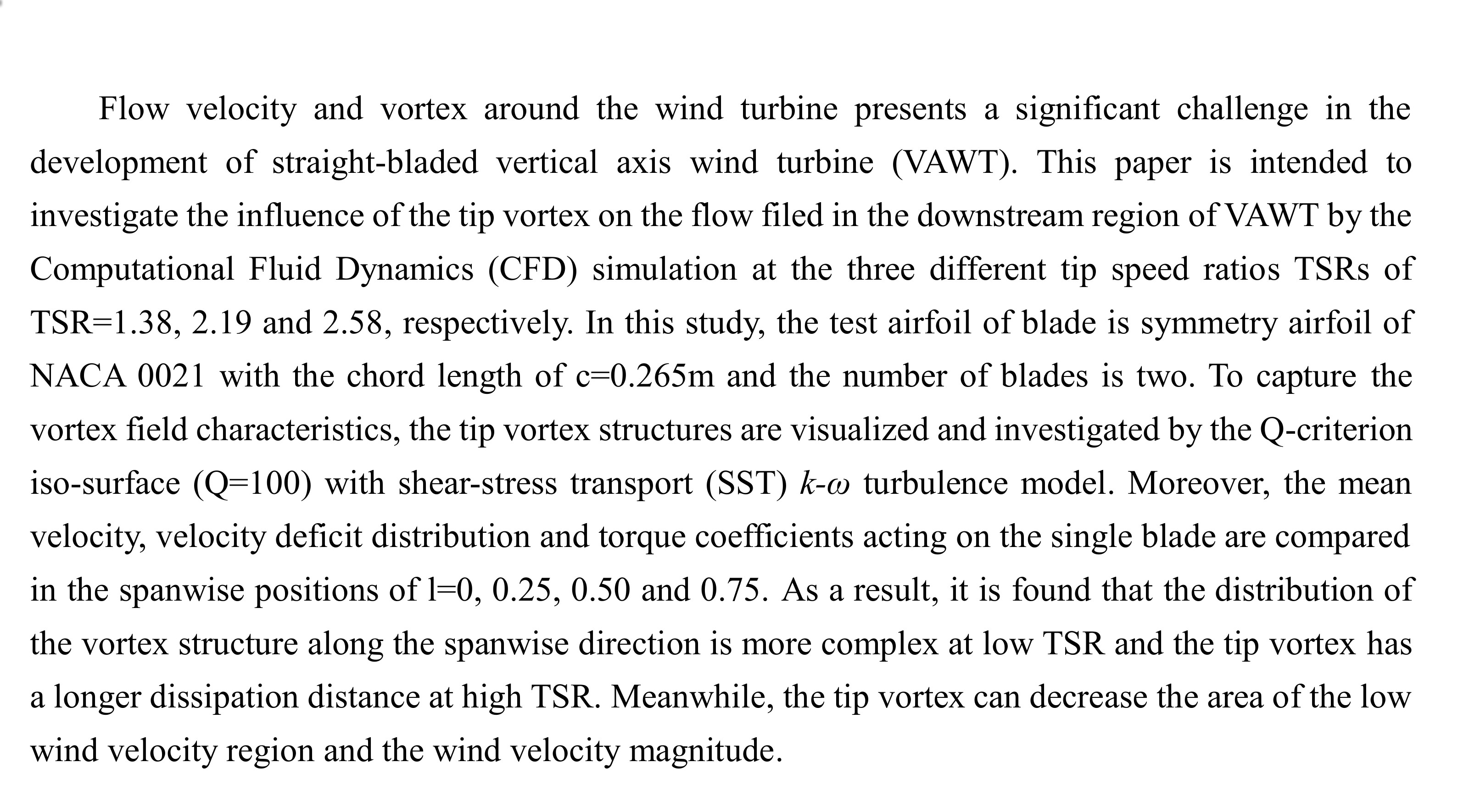
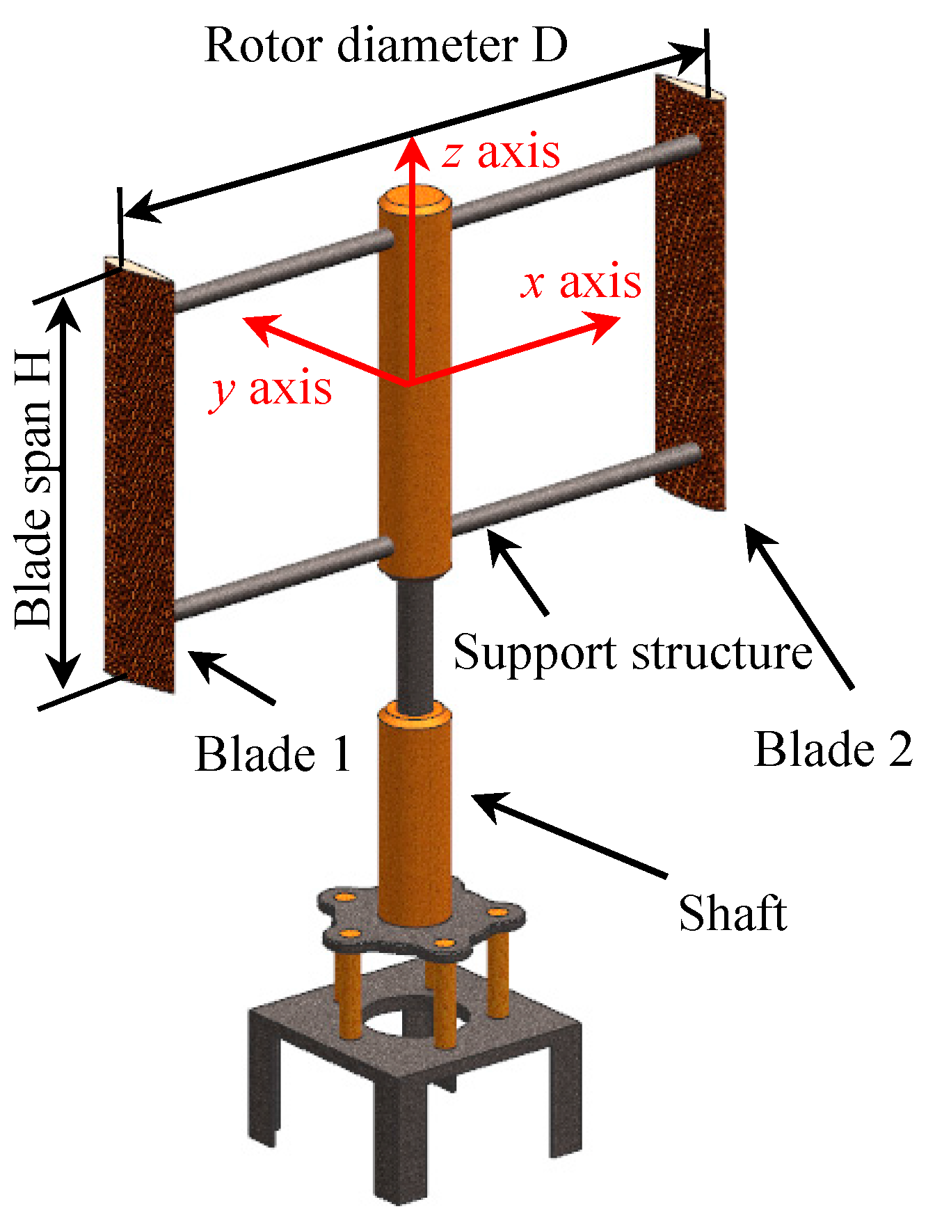
Figure 1 represents the main structure of a straight-bladed VAWT. The number of blades is two and the airfoil profile is a symmetric NACA 0021 with a chord length of 0.265 m. The rotor diameter of the wind turbine is R = 1.0 m and the blade span is H = 1.2 m. Therefore, the VAWT in this study gives a projected area of 2.4 m2 and a turbine aspect ratio of 1.67. The blade pitch angle is set to 6°, for which the wind turbine has the maximum power coefficient at the mainstream velocity of 8.0 m/s. Regarding the description of this wind turbine, more details of the specification can be found in the publications of Li et al. [13,15,34]. In order to reduce the computational efforts, the support structure is neglected during the inspection of the tip vortex effects on the flow field of the VAWT. Figure 2 illustrates a top view of the VAWT and the wind velocity measurement positions in the mainstream direction (x axis). The rotation direction of blade is clockwise from the top side view. In Figure 2, the blade 1 is located at the azimuth angle of θ = 30°. In order to study the influence of the tip vortex on the downstream region, the velocity is investigated at the internal region of the rotor (x/R = 0 and 0.5) and the near-wake of wind turbine (x/R = 1.0, 1.5 and 2.0). Moreover, to examine the evolution process of tip vortex on the downstream region of wind turbine, the each wake section is distributed in the spanwise cross-sections of l = 0, 0.25, 0.50 and 0.75 (l = z/(H/2)).
3.2. Mesh Strategy
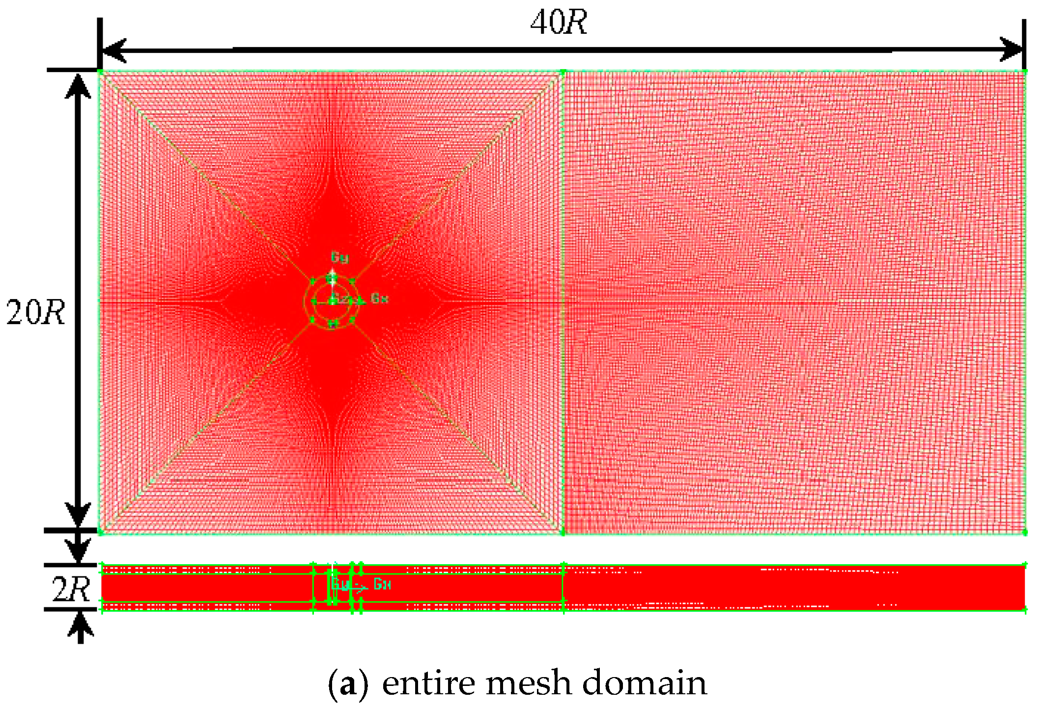
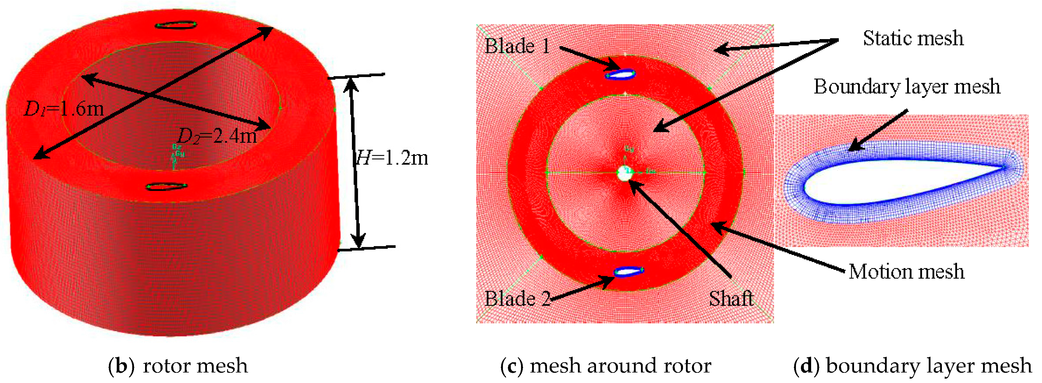
Figure 3 shows the computational domain of the VAWT. In Figure 3a, to reduce the blockage effects and disturbances of outer boundaries, the computational region is set at L = 20D in streamwise length, W = 10D in crosswind width and H0 = D (H0 > H = 0.6D) at spanwise height. As shown in Figure 3c, the computational region of VAWT is divided into the rotating domain and the static domain. In Figure 3b, the inside, outside diameters and height of rotating domain are D1 = 1.6 m, D2 = 2.4 m and H = 1.2 m. The mesh includes close to 3.5 million and 1.5 million computational cells in the whole numerical region and the rotating domain, respectively. To accurately investigate the formation of the tip vortex, the mesh is concentrated in the vicinity of the rotor blade. The elements and the type of static region are set to the Hex and the Map, respectively. The elements and the type of motion region are set to the Hex/Wedge and the Cooper. Figure 3d illustrates the boundary layer of blade surface and the refined mesh around blade, because the mesh intensity has a significant effect on the evolution of vortex. The Reynolds number is a low Reynolds number and approximately 2.89 × 10⁵. Therefore, it is beneficial to perform CFD simulations when y+ is less than 1. In addition, it has been calculated by Van. [35] and Lei et al. [36] that it can meet the requirement of y+ < 1 when the depth is 0.02 m, the growth factor is 1.25 and the first row is 2 × 10⁻⁵.
3.3. Boundary Conditions
In Figure 4 the boundary conditions that are applied in the CFD simulations are labeled. The boundary condition of the inlet of numerical region adopts the VELOCITY-INLET and the outlet of numerical region adopts the PRESSURE-OUTLET. The boundary condition of the borders of computational region is set at WALL. Moreover, the angular velocities of CFD simulations in the rotating domain are set at ω = −11.04, −17.58 and −20.73, respectively. In the cases of ω = −11.04, −17.58 and −20.73, the time step sizes are set to t = 0.00316 s, 0.00198 s and 0.00168 s. The number of time steps is set to N = 540. In addition, the INTERFACE is selected as the boundary condition of borders between the rotating domain and the static domain. According to the performance of server and precision of CFD simulation, the solution of implicit unsteady and segregated flow is adopted. For the discretization of Navier-Stokes equation, the difference equations of second order scheme are adopted and the coupling equation is solved by a simple method.
3.4. Wind Tunnel Experimental Measurements
Wind tunnel measurements have been performed in an open test section of a circular type wind tunnel with the inner diameter of 3.6 m. Similar to the simulation conditions, the mainstream wind velocity is performed at 8.0 m/s and the tip speed ratios are set at TSRs = 1.38, 2.19 and 2.58. Wind velocity distribution around the wind turbine is measured by a LDV system with a maximum output power of 4.0 W. However, the limitation of this experiment is that the measurements are performed only at the center cross-section of l = 0, rather than l = 0, 0.25, 0.50 and 0.75. Detailed descriptions of the wind tunnel experiments can also be found in Li et al. [34].
4. Data Processing Method
The Reynolds number (Re) is a non-dimensional number that can be used to characterize the fluid flow. It is used to distinguish the flow of fluid in laminar and turbulent flow. In this study, the Reynolds number can be expressed as [16,37]:
where, U and v represent the wind velocity and kinematic eddy viscosity. The TSR which is an important parameter to describe the characteristics of wind turbine can be defined as [7,24,38]:
The torque coefficient CQ of the rotor which reflects the wind turbine performance can be expressed as [16,29,39]:
Since the advent of Q-criteria, it has been widely used to investigate the results of CFD simulations. In this study, vortex around the rotor is detected by the iso-surface of a given Q value. Q is the second scalar invariant of velocity derivative tensor and can be defined as an incompressible flow [40]:
where, Wij and Sij are the symmetric and the unsymmetric parts of velocity derivative tensor.
5. Results and Discussion
As mentioned in the Introduction section, the wind velocity, pressure distribution and torque can be measured by wind tunnel experiments. However, the vortex structure is very difficult to capture in wind tunnel experiments. CFD simulation is a good method to capture the vortex structure. In this paper, CFD simulation is the main research method where the aim is to study the effect of tip vortex on the wind turbine wake. The results are verified by the experimental data from the available literature.
Figure 5 describes the fluctuations of the mean wind velocity at the azimuth angle of 0° < θ < 360° along x axis direction (y/R = 0, TSR = 2.19). C-l and E-l represent the mean wind velocity calculated by CFD simulations and measured by wind tunnel experiment in different cross-sections of l. As shown in the figure, in the blade center position, the curve of simulation results indicate a good agreement with the wind tunnel experimental data when the x/R is below −0.5. However, in the region of −0.5 < x/R < 0.5, the mean wind velocity of simulation results is slightly smaller than that of wind tunnel experiments. It seems that the support structure of VAWT is neglected in the CFD simulations. The vortex, which is generated by the support structure, increases the turbulence intensity in the rotating plane of wind turbine (−0.5 < x/R < 0.5). Therefore, compared with the CFD simulations, the high turbulence intensity facilitates the instantaneous recovery of wind velocity at −0.5 < x/R < 0.5 in the wind tunnel measurements. In the case of C-l = 0, it is still noteworthy that the mean wind velocity in the near-wake of VAWT computed by CFD simulations is larger than that of experiment data at x/R > 0.5. The vorticity is dragged along with the airfoil, resulting in a support structure vortex interaction in the near-wake of wind turbine. Thus, the vortex which is shed from the support structure, increases the mean wind velocity in the near-wake of the wind turbine. Remarkably, the mean wind velocity in the mainstream direction increases with the increase of C-l due to the tip vortex effect. Therefore, the mean wind velocity shows a large value near the blade tip and a small value near the C-l = 0.
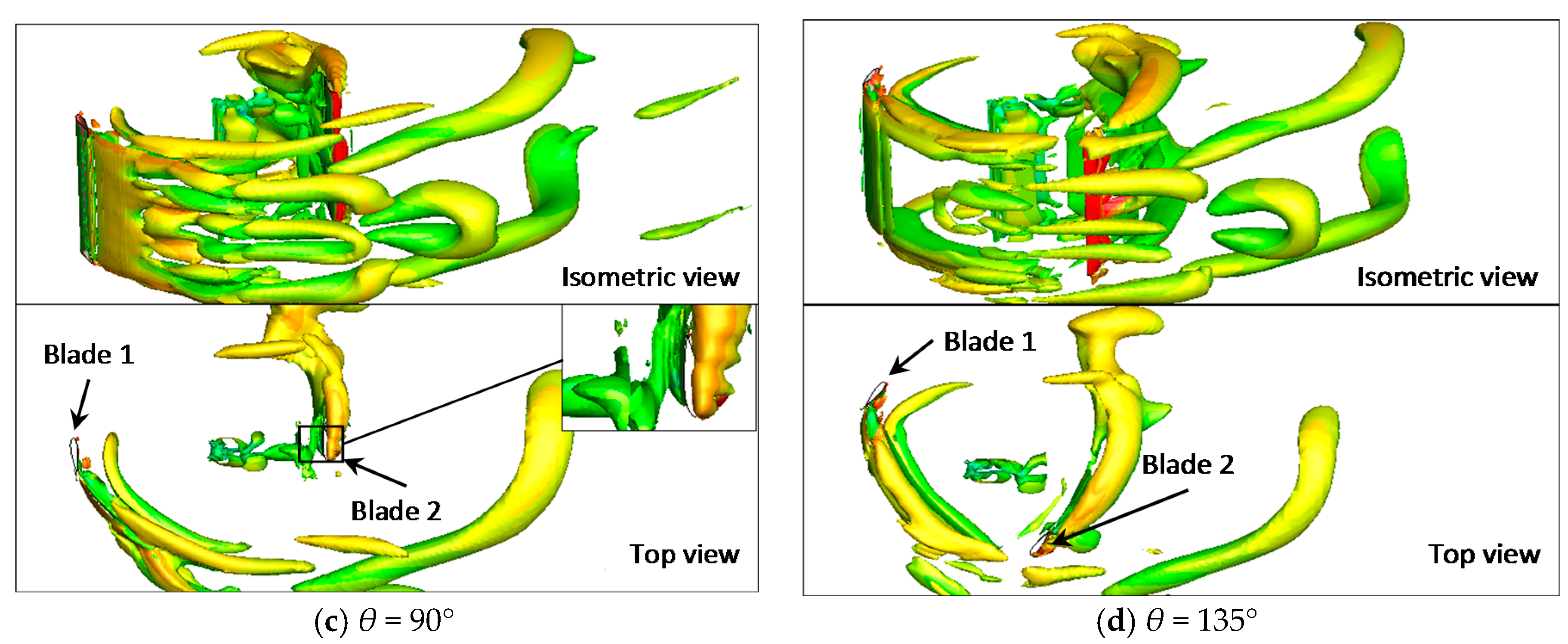
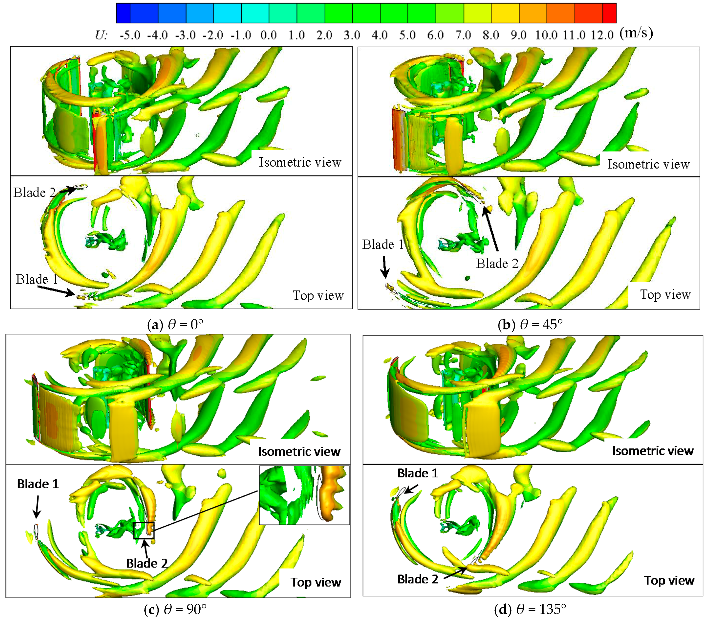
Figure 6, Figure 7 and Figure 8 show the vortex structure of rotor at the tip speed ratios of TSRs = 1.38, 2.19 and 2.58, when the azimuth angles are θ = 0°, 45°, 90° and 135°, respectively. The vortex structure is described by Q-criterion iso-surface and contour of resultant wind velocity. As shown in Figure 7a, vortex A, vortex B and vortex C represent the shedding vortex of the blade, tip vortex and vortex generated by the rotor shaft, respectively. The angle of attack is changed periodically during rotation and generates the dynamic stall phenomenon which involves a series of fluid flow attachments, separations and reattachments that occurred on the airfoil surface. The flow is characterized by the shedding vortex which will be generated as airflow shedding from the blade. The principle of tip vortex is the airflow on the positive pressure surface of blade around the tip of blade to the negative pressure surface of blade. Similar conclusion of generation mechanism of vorticities including tip vortex can be found in the studies of Ferreira et al. [19] in 2009 with PIV experiments and Li et al. [41] in 2016 with pressure measurements. Moreover, from Figure 6c, Figure 7c and Figure 8c which include local enlarged views, it is clearly observed that vortex B around the rotor shaft can affect the vortex C around the blade. The vortex of rotor is mainly composed of shedding vortex, tip vortex and vortex produced by the shaft. However, compared with other vortices, the tip vortex has a longer dissipation distance. It is noted that the vortex structure is asymmetrical relative to the y-z plane. The tip vortex mainly originates in the region of azimuth angles of −90° < θ < 90° due to the large angle of attack. Moreover, the shaft that is often overlooked in CFD simulations also has certain influence on the rotor, because the vortex produced by the shaft bypasses the blade surface around θ = 270° (see Figure 6c, Figure 7c and Figure 8c).
Compared with the TSRs = 1.38 and 2.19, the tip vortex at TSR = 2.58 has the longest dissipation distance and simplest structure, which demonstrates that a higher TSR has a more significant impact on the wind turbine wake. In addition, the tip vortex and the shedding vortex at low TSR of 1.38 have more irregular structures than that at a higher TSR, especially in the spanwise direction. This also implies that the airflow in the downstream region is more complex at a lower TSR. The interaction between the tip vortex generated by blade 1 and blade 2 at TSR = 2.58 is more intensive than that at TSRs = 1.38 and 2.19. In particular, the interaction near blade 2 at the azimuth angles of θ = 90° and 135° is stronger than that at the azimuth angles of θ = 0° and 45°. Indeed, the TSR has a strong effect on the evolution of the tip vortex, and the tip vortex induces the complex flow field in the downstream region.
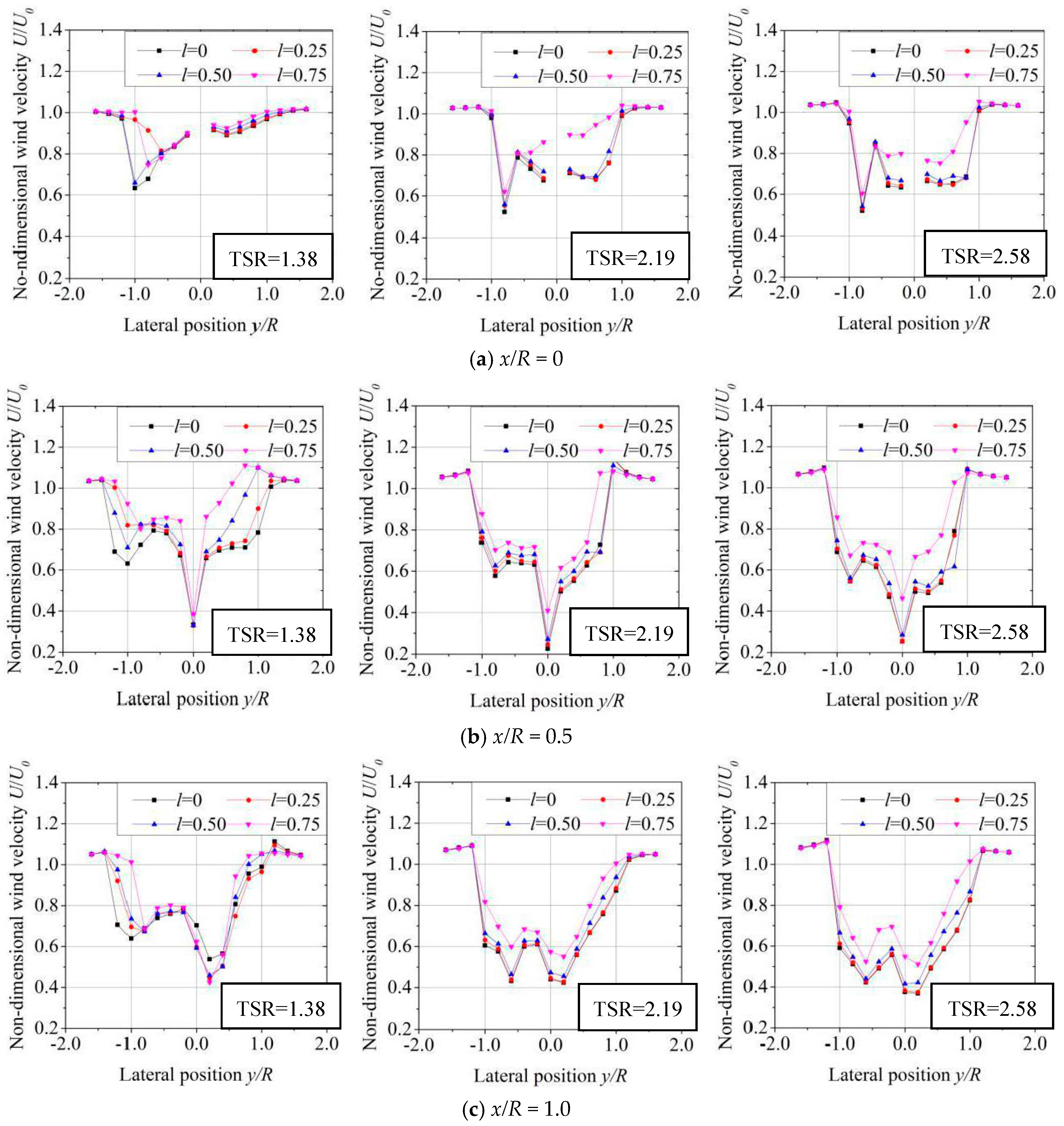
Figure 9 depicts the fluctuations of mean wind velocity in the cross-sections of l = 0, 0.25, 0.50 and 0.75. In this figure, the azimuth angle is 0° < θ < 360°, the tip speed ratio is TSR = 2.19 and the longitudinal position is x/R = 0. The mean wind velocity of each point is the average value in the lateral direction of −1.6 < y/R < 1.6. The horizontal axis and the vertical axis represent the azimuth angle θ and the non-dimensional wind velocity U/U0, respectively. The fluctuation of mean wind velocity is two cycles at the azimuth angle of 0° ≤ θ ≤ 360°. Therefore, it is only necessary to analyze mean wind velocity at the azimuth angle of 0° ≤ θ < 180°.
As shown in Figure 9, the value of mean wind velocity increases with increase of l. It seems that the mean velocity in the section near the tip of blade is larger than that near the center of blade. As mentioned in Figure 6, the flow field is different at different azimuth angles and the fluctuation of the mean wind velocity are also different for different cross-sections of l = 0, 0.25, 0.50 and 0.75. It is considered that the influence of the blade vortex is greater when close to the tip of blade. Li et al. [29] in 2016 also obtained the similar results with the LDV measurement in a large wind tunnel. Figure 10 illustrates the low wind velocity contours in different cross-sections of l = 0, 0.25, 0.50 and 0.75 when the azimuth angle is θ = 90°. As shown in the figure, the areas of low velocity region have the minimum in the cross-section of l = 0 and the area decreases with the increase of l at three different TSRs. There are three main reasons for this phenomenon: Firstly, the influence of tip vortex on airflow around the blade increases with the increase of l. Secondly, the blockage effect of rotor is small near the blade tip. Finally, the interaction between the free-airflow passing through the blade tip and the airflow bypassing the blade surface is strong near the blade tip. In addition, the areas of low wind velocity regions at TSR = 2.58 are larger than that of TSRs = 1.38 and 2.19 in all the cross-sections. Therefore, in the case of the low tip speed ratio, the effect of tip vortex on the wind velocity is larger and the wind velocity in the wind turbine wake has a faster recovery than that of a higher TSR.
To examine the wind velocity deficit characteristics of the wind turbine wake, the fluctuations of wind velocity are shown in Figure 11 in the downstream positions of x/R = 0, 1.0, 2.0, 3.0 and 4.0. As shown in this figure, the velocity field is compared at the cross-sections of l = 0, 0.25, 0.50 and 0.75 when the azimuth angle is θ = 0° and the tip speed ratios are TSRs = 1.38, 2.19 and 2.58. It can be observed that when the cross-section is l = 0, the wind velocity has the minimum value in the cases of x/R = 0, 0.25, 0.50 and 0.75. And the magnitude of wind velocity decreases with the increase of l. In the case of TSR = 1.38, the difference between the wind velocity of l = 0 and 0.75 increases and then decreases with the increase of the x/R. However, in the cases of TSRs = 2.19 and 2.58, the difference increases with the increase of the x/R (0 < x/R < 2.0).
In the previous chapters, the effect of tip vortex on the flow field has been discussed at the azimuth angle of θ = 90° in the downstream region. In this chapter, the mean wind velocity deficit at azimuth angle of θ = 90° is demonstrated in Figure 12. The results are analyzed in different cross-sections of l = 0, 0.25, 0.50 and 0.75 at TSRs = 1.38, 2.19, 2.58. The large mandatory circle and the small solid circle represent the rotating track of rotor and the shaft of the wind turbine, respectively. In this study, the length of arrow indicates the magnitude of wind velocity in the mainstream direction. The left end point of arrow is the point of U = 0 m/s. The shaded area which shows the wind velocity deficit is formed from the curve connected by the right endpoint of arrow and the straight line of U = 8.0 m/s. As shown in the figure, the wind velocity deficit show the minimum value when the l is 0.75 in the cases of TSRs = 1.38, 2.19 and 2.58. When the value of TSR is 2.58, the wind velocity deficit in l = 0 is about twice in l = 0.75. The wind velocity deficit increases with the decrease of TSR. Moreover, the wind velocity deficit of TSR = 1.38 is smaller than that of TSRs = 2.19 and 2.58 at each spanwise section. The maximum of the wind velocity deficit is shown in the wake positions of x/R = 2.5, 2.5, 2.0 and 1.5, corresponding to the l of 0, 0.25, 0.50 and 0.75, respectively. Therefore, the recovered distance of wind velocity in l = 0.75 is shorter than that in l = 0 due to the tip vortex effect.
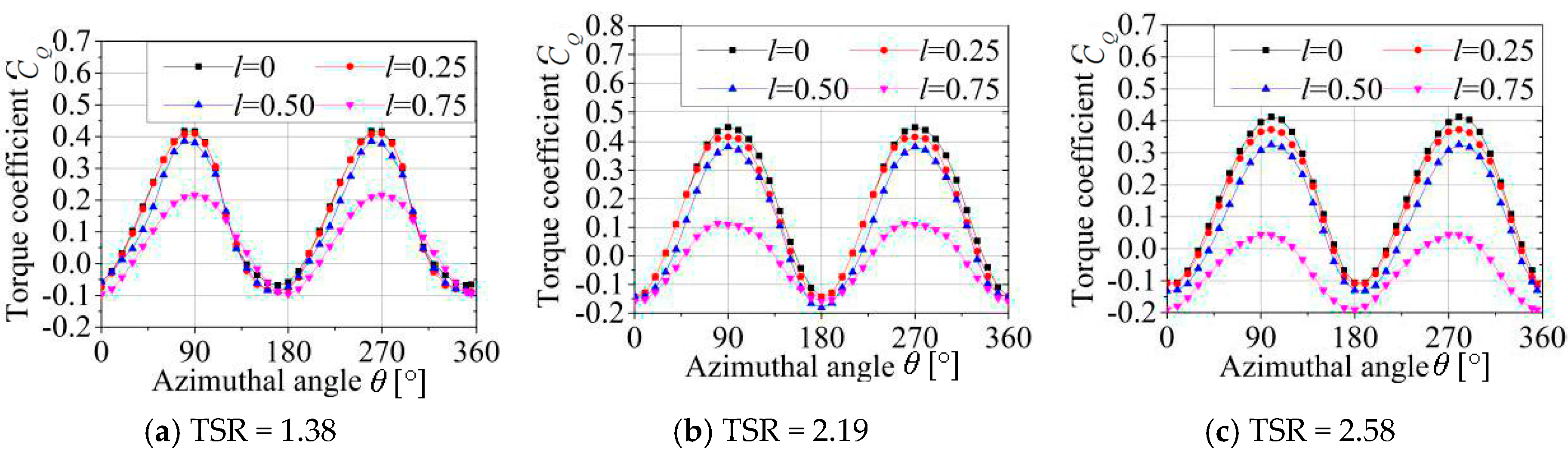
Figure 13a–c depict the fluctuations of the torque coefficient during ration at the different spanwise sections of l = 0, 0.25, 0.50 and 0.75 when the tip speed ratios are TSRs = 1.38, 2.19 and 2.58. From these figures, in the case of TSR = 1.38, the maximum value of the torque coefficient in l = 0 (CQ = 0.417) is larger than that of l = 0.75 (CQ = 0.206). Therefore, the tip vortex has a larger effect on the aerodynamic characteristics of the rotor at a higher TSR. When the blade passes through the azimuth angle of θ = 90°, the torque coefficients have the maximum value at different spanwise sections. In the case of l = 0, the maximum values of torque coefficient are 0.417, 0.450 and 0.412 for the TSRs of 1.38, 2.19 and 2.58, respectively. In the case of l = 0.75, the maximum values of torque coefficient are 0.206, 0.114 and 0.044 at TSRs = 1.38, 2.19 and 2.58, respectively. The torque coefficients show the small value at the downstream region. The minimum value of torque coefficient is found in l = 0 at TSR = 2.19, while the minimum value of CQ is found in l = 0.75 at the TSR = 2.58 and smaller than that of TSR = 2.19. It is mainly considered that the tip vortex of the blade has a larger influence at a higher TSR (see Figure 7, Figure 8 and Figure 9). The similar result also has a good agreement with the study of Li et al. [42] in 2017.
6. Conclusions
This study is aimed at investigating the effect of tip vortex on the downstream region of VAWT in the different spanwise cross-sections of l = 0, 0.25, 0.50 and 0.75. Firstly, the velocity fields are investigated by CFD simulations and LDV measurements. Then, to capture the vortex evolution, the tip vortex on the flow field of straight-bladed VAWT is compared at three different TSRs with numerical investigation. The flow field characteristics can be summarized as follows:
- (1)
- The vortex which is generated by the support structure increases the turbulence intensity in the rotating plane of wind turbine (–0.5 < x/R < 0.5). Meanwhile, the mean wind velocity in the mainstream direction increase with the increase of C-l due to the tip vortex effect.
- (2)
- Compared with other vortices, the tip vortex has a longer dissipation distance. It is noted that the vortex structure is an asymmetrical relative to the y-z plane. The tip vortex mainly originates in the region of azimuth angles of −90° < θ < 90° due to the large angle of attack.
- (3)
- The areas of low velocity region have the minimum in the cross-section of l = 0 and the area decreases with the increase of l at three different TSRs. In addition, the areas of low wind velocity regions at TSR = 2.58 are larger than that of TSRs = 1.38 and 2.19 in all the cross-sections. Therefore, in the case of the low tip speed ratio, the effect of tip vortex on the wind velocity is larger and the wind velocity in the wind turbine wake has a faster recovery than that of a higher TSR.
- (4)
- The torque coefficients show the maximum value at about the azimuth angle of θ = 90° on the upstream region. In the case of l = 0, the maximum values of torque coefficient are 0.417, 0.450 and 0.412 for the TSRs of 1.38, 2.19 and 2.58, respectively. In the case of l = 0.75, the maximum values of torque coefficient are 0.206, 0.114 and 0.044 at TSRs = 1.38, 2.19 and 2.58, respectively.
Acknowledgments
This work is supported by the National Natural Science Foundation of China (No. 51765050) and Key Research Project of Shandong Province of China (No. 2017GGX40124).
Author Contributions
Yanzhao Yang and Yanfeng Zhang conducted the data collection and wrote the manuscript; Ho Jinyama revised the manuscript; Zhiping Guo and Qingan Li contributed analysis tools and technical guidance.
Conflicts of Interest
The authors declare no conflict of interest.
Nomenclature
| c | Airfoil chord length [m] |
| CQ | Rotor torque coefficient |
| F1 | Hybrid function [k-ω] |
| F2 | Second hybrid function [SST k-ω] |
| H | Spanwise length [m] |
| H0 | Numerical region height [m] |
| k | Turbulent kinetic energy [m2/s2] |
| l | Section perpendicular to the z axis [=z/(H/2)] |
| L | Numerical region length [m] |
| R | Rotor radius [m] |
| Re | Reynolds number [=Uc/v] |
| S | Tension constant |
| U | Local wind velocity [m/s] |
| U0 | Mainstream velocity [m/s] |
| W | Numerical region width [m] |
| x | Longitudinal coordinate [m] |
| y | Lateral coordinate [m] |
| z | Vertical coordinate [m] |
| α | Angle of attack [°] |
| μt | Eddy viscosity [(N·s)/m2] |
| ν | Kinematic eddy viscosity [m2/s] |
| θ | Azimuth angle [°] |
| ρ | Air density [kg/m3] |
| ω | Specific turbulent dissipation rate [s−1] |
| ω0 | Angular velocity [rad/s] |
| ψ1 | Auxilary relation |
| CFD | Computational fluid dynamics |
| NACA | National Advisory Committee for Aeronautics |
| HAWT | Horizontal axis wind turbine |
| SST | Shear stress transport |
| TSR | Tip speed ratio [=(Rω)/U0] |
| VAWT | Vertical axis wind turbine |
References
- Chiras, D. Wind Power Basics: A Green Energy Guide; New Society Publishers: Vancouver, BC, Canada, 2010. [Google Scholar]
- Jefferson, M. Sustainable energy development: Performance and prospects. Renew. Energy 2006, 31, 571–582. [Google Scholar] [CrossRef]
- Ashwill, T.D.; Sutherland, H.J.; Berg, D.E. A Retrospective of VAWT Technology; Sandia National Laboratories: Albuquerque, NM, USA, 2012. [Google Scholar]
- Li, Q.; Kamada, Y.; Maeda, T.; Murata, J.; Iida, K.; Okumura, Y. Fundamental study on aerodynamic force of floating offshore wind turbine with cyclic pitch mechanism. Energy 2016, 99, 20–31. [Google Scholar] [CrossRef]
- Burtnick, J.; Fairbanks, R.; Gross, F.; Lin, E.; McCrone, B.; Osmond, J. Placement of Small Vertical Axis Wind Turbine to Maximize Power Generation Influenced by Architectural and Geographic Interfaces in Urban Areas; University of Maryland: College Park, MD, USA, 2015. [Google Scholar]
- Ryan, K.J.; Coletti, F.; Elkins, C.J.; Dabiri, J.O.; Eaton, J.K. Three-dimensional flow field around and downstream of a subscale model rotating vertical axis wind turbine. Exp. Fluids 2016, 57, 1–15. [Google Scholar] [CrossRef]
- Lei, H.; Zhou, D.; Bao, Y.; Li, Y.; Han, Z. Three-dimensional Improved Delayed Detached Eddy Simulation of a two-bladed vertical axis wind turbine. Energy Convers. Manag. 2017, 133, 235–248. [Google Scholar] [CrossRef]
- Beri, H.; Yao, Y. Double multiple streamtube model and numerical analysis of vertical axis wind turbine. Energy Power Eng. 2011, 3, 262–270. [Google Scholar] [CrossRef]
- Fukudome, K.; Watanabe, M.; Iida, A.; Mizuno, A. Separation control of high angle of attack airfoil for vertical axis wind turbines. AIAA J. 2005, 50, 3. [Google Scholar]
- McLaren, K.; Tullis, S.; Ziada, S. Computational fluid dynamics simulation of the aerodynamics of a high solidity, small-scale vertical axis wind turbine. Wind Energy 2012, 15, 349–361. [Google Scholar] [CrossRef]
- Hofemann, C.; Ferreira, C.S.; Van Bussel, G.J.; Van Kuik, G.A.; Scarano, F.; Dixon, K.R. 3D Stereo PIV Study of Tip Vortex Evolution on a Vawt; European Wind Energy Association EWEA: Brussels, Belgium, 2012. [Google Scholar]
- Sun, X.; Wang, Y.; An, Q.; Cao, Y.; Wu, G.; Huang, D. Aerodynamic performance and characteristic of vortex structures for Darrieus wind turbine. I. Numerical method and aerodynamic performance. J. Renew. Sustain. Energy 2014, 6, 043134. [Google Scholar] [CrossRef]
- Li, Q.; Maeda, T.; Kamada, Y.; Murata, J.; Furukawa, K.; Yamamoto, M. Investigation of power performance and wake on a straight-bladed vertical axis wind turbine with field experiments. Energy 2017, 142, 260–271. [Google Scholar] [CrossRef]
- Chen, Y.; Lian, Y. Numerical investigation of vortex dynamics in an H-rotor vertical axis wind turbine. Eng. Appl. Comput. Fluid Mech. 2015, 9, 21–32. [Google Scholar] [CrossRef]
- Li, Q.; Maeda, T.; Kamada, Y.; Murata, J.; Furukawa, K.; Yamamoto, M. Measurement of the flow field around straight-bladed vertical axis wind turbine. J. Wind Eng. Ind. Aerodyn. 2016, 151, 70–78. [Google Scholar] [CrossRef]
- Li, Q.; Maeda, T.; Kamada, Y.; Murata, J.; Yamamoto, M.; Ogasawara, T.; Kogaki, T. Study on power performance for straight-bladed vertical axis wind turbine by field and wind tunnel test. Renew. Energy 2016, 90, 291–300. [Google Scholar] [CrossRef]
- Posa, A.; Parker, C.M.; Leftwich, M.C.; Balaras, E. Wake structure of a single vertical axis wind turbine. Int. J. Heat Fluid Flow 2016, 61, 75–84. [Google Scholar] [CrossRef]
- Vittecoq, P. Dynamic stall: The case of the vertical axis wind turbine. J. Sol. Energy Eng. 1986, 108, 140–145. [Google Scholar]
- Ferreira, C. S.; van Kuik, G.; van Bussel, G.; Scarano, F. Visualization by PIV of dynamic stall on a vertical axis wind turbine. Exp. Fluids 2009, 46, 97–108. [Google Scholar] [CrossRef]
- Qin, N.; Howell, R.; Durrani, N.; Hamada, K.; Smith, T. Unsteady flow simulation and dynamic stall behaviour of vertical axis wind turbine blades. Wind Eng. 2011, 35, 511–527. [Google Scholar] [CrossRef]
- Lanzafame, R.; Mauro, S.; Messina, M. 2D CFD modeling of H-Darrieus wind turbines using a transition turbulence model. Energy Procedia 2014, 45, 131–140. [Google Scholar] [CrossRef]
- Buchner, A.J.; Lohry, M.W.; Martinelli, L. Dynamic stall in vertical axis wind turbines: Comparing experiments and computations. J. Wind Eng. Ind. Aerodyn. 2015, 146, 163–171. [Google Scholar] [CrossRef]
- Dunne, R. Dynamic Stall on Vertical Axis Wind Turbines; California Institute of Technology: Pasadena, CA, USA, 2016. [Google Scholar]
- Sun, X.; Wang, Y.; An, Q.; Cao, Y.; Wu, G.; Huang, D. Aerodynamic performance and characteristic of vortex structures for Darrieus wind turbine. II. The relationship between vortex structure and aerodynamic performance. J. Renew. Sustain. Energy 2014, 6, 043135. [Google Scholar] [CrossRef]
- Chatelain, P.; Duponcheel, M.; Caprace, D.G.; Marichal, Y.; Winckelmans, G. Vortex Particle-Mesh simulations of Vertical Axis Wind Turbine flows: From the blade aerodynamics to the very far wake. J. Phys. Conf. Ser. 2016, 753, 032007. [Google Scholar] [CrossRef]
- Thé, J.; Yu, H. A critical review on the simulations of wind turbine aerodynamics focusing on hybrid RANS-LES methods. Energy 2017, 138, 257–289. [Google Scholar]
- Li, Q.; Maeda, T.; Kamada, Y.; Shimizu, K.; Ogasawara, T.; Nakai, A.; Kasuya, T. Effect of rotor aspect ratio and solidity on a straight-bladed vertical axis wind turbine in three-dimensional analysis by the panel method. Energy 2017, 121, 1–9. [Google Scholar] [CrossRef]
- Li, Q.; Maeda, T.; Kamada, Y.; Murata, J.; Kawabata, T.; Shimizu, K.; Kasuya, T. Wind tunnel and numerical study of a straight-bladed Vertical Axis Wind Turbine in three-dimensional analysis (Part II: For predicting flow field and performance). Energy 2016, 104, 295–307. [Google Scholar] [CrossRef]
- Li, Q.; Maeda, T.; Kamada, Y.; Murata, J.; Kawabata, T.; Shimizu, K.; Kasuya, T. Wind tunnel and numerical study of a straight-bladed vertical axis wind turbine in three-dimensional analysis (Part I: For predicting aerodynamic loads and performance). Energy 2016, 106, 443–452. [Google Scholar] [CrossRef]
- Chen, T.; Xia, Y.; Liu, W.; Liu, H.; Sun, L.; Lee, C. A Hybrid Flapping-Blade Wind Energy Harvester Based on Vortex Shedding Effect. J. Microelectromech. Syst. 2016, 25, 845–847. [Google Scholar] [CrossRef]
- Parker, C.M.; Hummels, R.; Leftwich, M.C. Flow measurement behind a pair of vertical-axis wind turbines. In Proceedings of the 70th Annual Meeting of the APS Division of Fluid Dynamics, Denver, CO, USA, 19–21 November 2017. [Google Scholar]
- Menter, F.R. Two-equation eddy-viscosity turbulence models for engineering applications. AIAA J. 1994, 32, 1598–1605. [Google Scholar] [CrossRef]
- Ferreira, S.C.J. The Near Wake of the VAWT: 2D and 3D Views of the VAWT Aerodynamics. Ph.D. Thesis, Delft University of Technology, Delft, The Netherlands, October 2009. [Google Scholar]
- Li, Q.; Maeda, T.; Kamada, Y.; Murata, J.; Furukawa, K.; Yamamoto, M. The influence of flow field and aerodynamic forces on a straight-bladed vertical axis wind turbine. Energy 2016, 111, 260–271. [Google Scholar] [CrossRef]
- Van de Wal, H.J.B. Design of a Wing with Boundary Layer Suction. Master’s Thesis, Delft University of Technology, Delft, The Netherlands, August 2010. [Google Scholar]
- Lei, H.; Zhou, D.; Lu, J.; Chen, C.; Han, Z.; Bao, Y. The impact of pitch motion of a platform on the aerodynamic performance of a floating vertical axis wind turbine. Energy 2017, 119, 369–383. [Google Scholar] [CrossRef]
- Li, Q.; Maeda, T.; Kamada, Y.; Murata, J.; Shimizu, K.; Ogasawara, T.; Kasuya, T. Effect of solidity on aerodynamic forces around straight-bladed vertical axis wind turbine by wind tunnel experiments (depending on number of blades). Renew. Energy 2016, 96, 928–939. [Google Scholar] [CrossRef]
- Valappil, D.K.; Somasekharan, N.; Krishna, S.; Laxman, V.; Kishore, V.R. Influence of Solidity and Wind Shear on the Performance of VAWT using a Free Vortex Model. Int. J. Renew. Energy Res. (IJRER) 2017, 7, 787–796. [Google Scholar]
- Heo, Y.G.; Choi, K.H.; Kim, K.C. CFD and experiment validation on aerodynamic power output of small vawt with low tip speed ratio. J. Korean Soc. Mar. Eng. 2016, 40, 330–335. [Google Scholar] [CrossRef]
- Lu, J.; Tang, H.; Wang, L.; Peng, F. A novel dynamic coherent eddy model and its application to LES of a turbulent jet with free surface. Sci. Chin. Phys. Mech. Astron. 2010, 53, 1671–1680. [Google Scholar] [CrossRef]
- Li, Q.; Maeda, T.; Kamada, Y.; Murata, J.; Furukawa, K.; Yamamoto, M. Effect of number of blades on aerodynamic forces on a straight-bladed vertical axis wind turbine. Energy 2015, 90, 784–795. [Google Scholar] [CrossRef]
- Li, Q.; Maeda, T.; Kamada, Y.; Hiromori, Y.; Nakai, A.; Kasuya, T. Study on stall behavior of a straight-bladed vertical axis wind turbine with numerical and experimental investigations. J. Wind Eng. Ind. Aerodyn. 2017, 164, 1–12. [Google Scholar] [CrossRef]
Figure 1.
Geometric model of straight-bladed VAWT in CFD simulations and wind tunnel experiments.

Figure 2.
Top view of VAWT and measured positions of the wind velocity along the longitudinal direction of the rotor. The five red lines represent the measured positions of x/R = 0, 0.5, 1.0, 1.5 and 2.0, respectively.
Figure 2.
Top view of VAWT and measured positions of the wind velocity along the longitudinal direction of the rotor. The five red lines represent the measured positions of x/R = 0, 0.5, 1.0, 1.5 and 2.0, respectively.

Figure 3.
Numerical region and mesh strategy for the VAWT: (a) show entire mesh domain, (b) rotor mesh, (c) mesh around rotor and (d) boundary layer mesh, respectively.
Figure 3.
Numerical region and mesh strategy for the VAWT: (a) show entire mesh domain, (b) rotor mesh, (c) mesh around rotor and (d) boundary layer mesh, respectively.


Figure 4.
Boundary conditions of the numerical region of the CFD simulation and cross-sections of l = 0, 0.25, 0.50 and 0.75.
Figure 4.
Boundary conditions of the numerical region of the CFD simulation and cross-sections of l = 0, 0.25, 0.50 and 0.75.
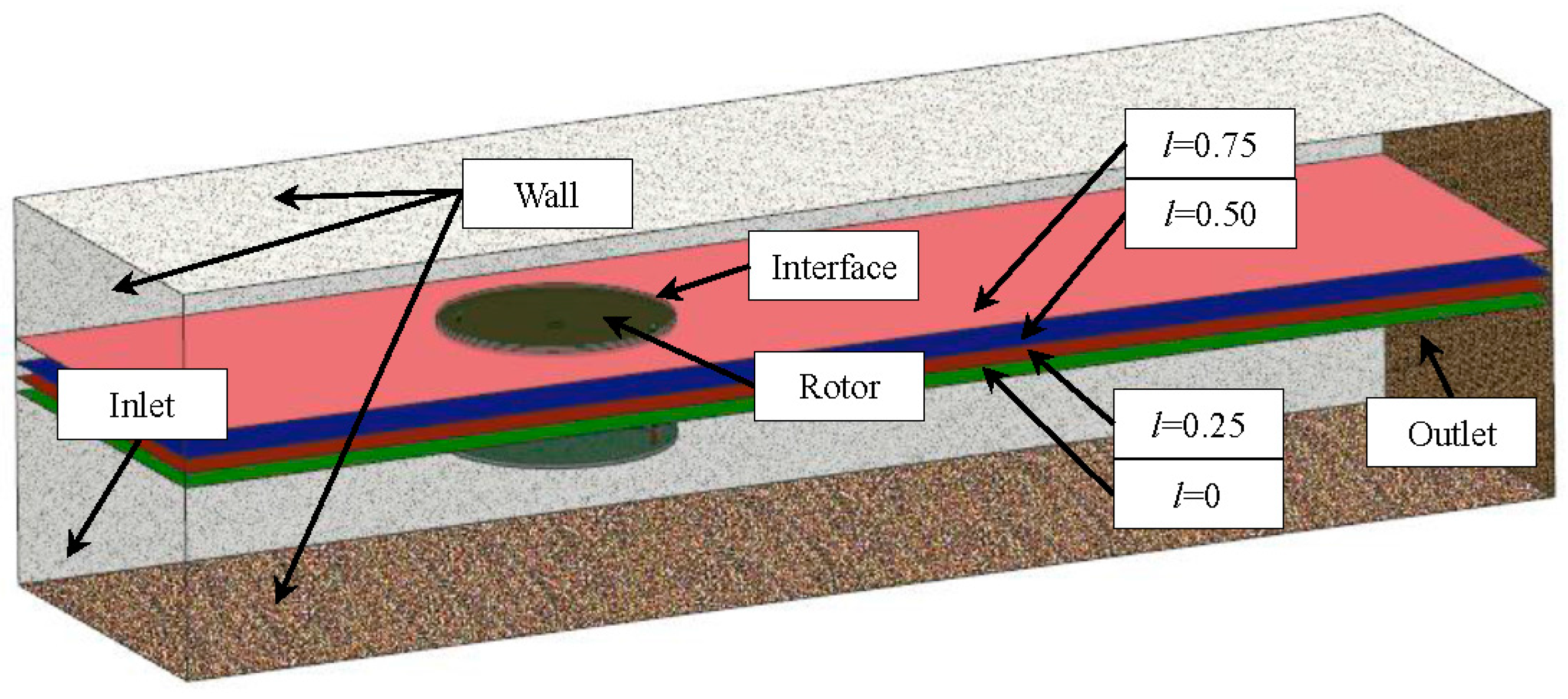
Figure 5.
Fluctuations of mean wind velocities for different cross-sections of l = 0, 0.25, 0.50 and 0.75 are compared in cross-section of l = 0 at TSR = 2.19 by CFD simulations and wind tunnel experiments.
Figure 5.
Fluctuations of mean wind velocities for different cross-sections of l = 0, 0.25, 0.50 and 0.75 are compared in cross-section of l = 0 at TSR = 2.19 by CFD simulations and wind tunnel experiments.
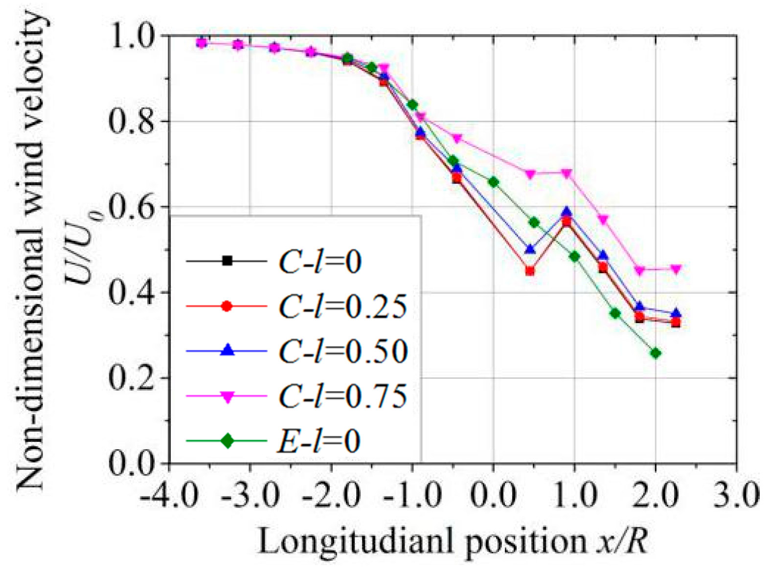
Figure 6.
Q-criterion iso-surface of vortex structure for rotor with the azimuth angle of (a) θ = 0°, (b) θ = 45°, (c) θ = 90° and (d) θ = 135° at TSR = 1.38. Contour of Q-criterion iso-surface depicts the wind velocity of U.
Figure 6.
Q-criterion iso-surface of vortex structure for rotor with the azimuth angle of (a) θ = 0°, (b) θ = 45°, (c) θ = 90° and (d) θ = 135° at TSR = 1.38. Contour of Q-criterion iso-surface depicts the wind velocity of U.
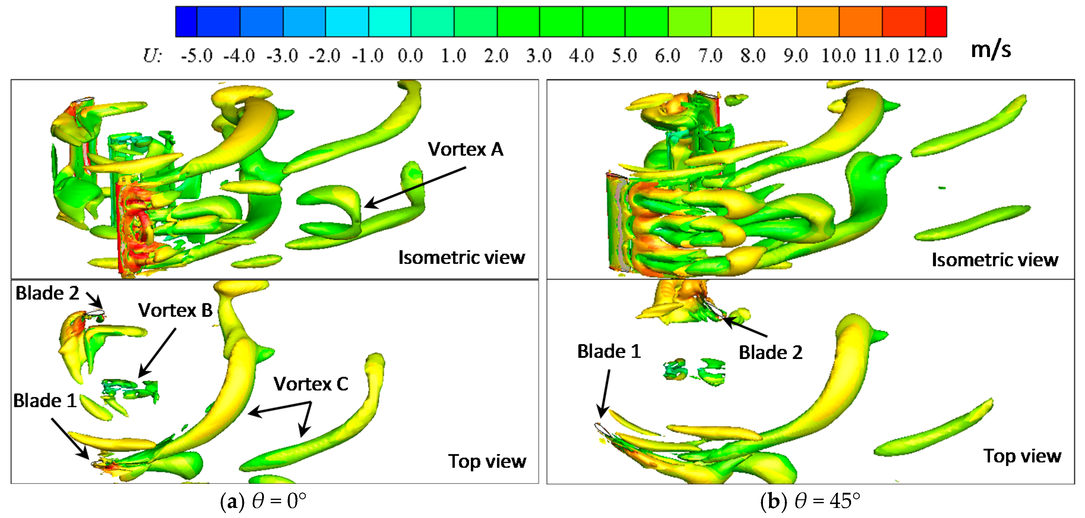

Figure 7.
Q-criterion iso-surface of vortex structure for rotor with the azimuth angle of (a) θ = 0°, (b) θ = 45°, (c) θ = 90° and (d) θ = 135° at TSR = 2.19. Contour of Q-criterion iso-surface depicts the wind velocity of U.
Figure 7.
Q-criterion iso-surface of vortex structure for rotor with the azimuth angle of (a) θ = 0°, (b) θ = 45°, (c) θ = 90° and (d) θ = 135° at TSR = 2.19. Contour of Q-criterion iso-surface depicts the wind velocity of U.
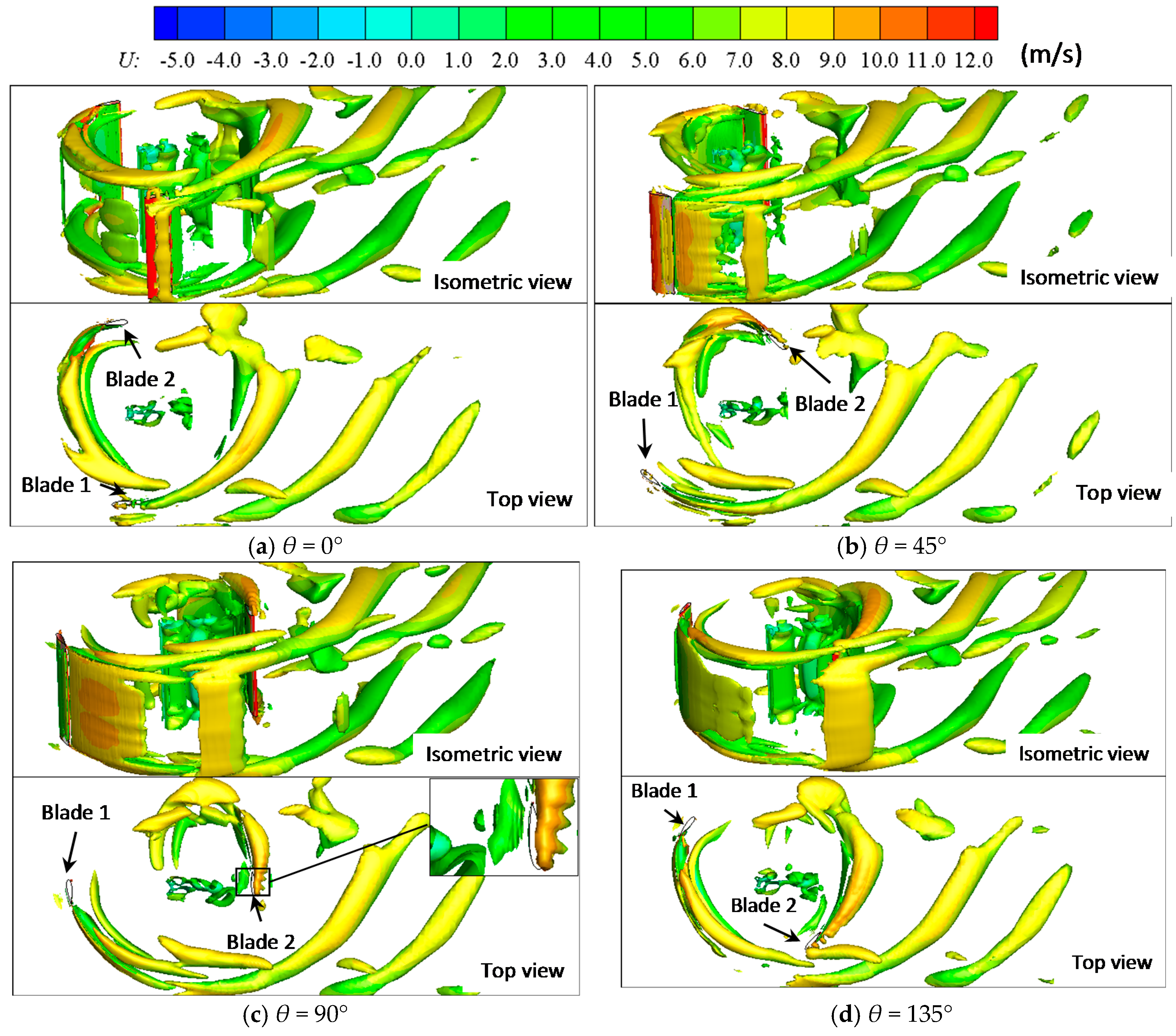
Figure 8.
Q-criterion iso-surface of vortex structure for rotor with the azimuth angle of (a) θ = 0°, (b) θ = 45°, (c) θ = 90° and (d) θ = 135° at TSR = 2.58. Contour of Q-criterion iso-surface depicts the wind velocity of U.
Figure 8.
Q-criterion iso-surface of vortex structure for rotor with the azimuth angle of (a) θ = 0°, (b) θ = 45°, (c) θ = 90° and (d) θ = 135° at TSR = 2.58. Contour of Q-criterion iso-surface depicts the wind velocity of U.

Figure 9.
Fluctuation of the mean wind velocity for different cross-sections of l = 0, 0.25, 0.50 and 0.75 during rotation. The mean wind velocity magnitudes are the average value in the range of −1.6 < y/R < 1.6 at x/R = 0.
Figure 9.
Fluctuation of the mean wind velocity for different cross-sections of l = 0, 0.25, 0.50 and 0.75 during rotation. The mean wind velocity magnitudes are the average value in the range of −1.6 < y/R < 1.6 at x/R = 0.
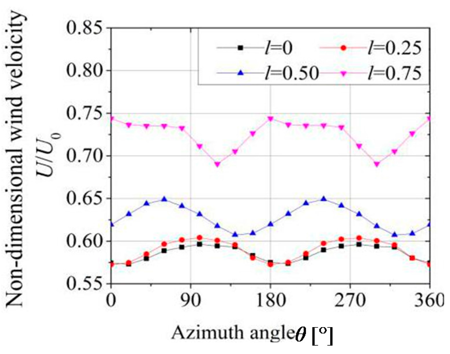
Figure 10.
Comparison of contour of wind velocity between the different cross-sections of l = 0, 0.25, 0.50 and 0.75 at three different TSRs with the azimuth angle of θ = 90°: (a–c) show the contour of wind velocity of TSR = 1.38, 2.19 and 2.58, respectively.
Figure 10.
Comparison of contour of wind velocity between the different cross-sections of l = 0, 0.25, 0.50 and 0.75 at three different TSRs with the azimuth angle of θ = 90°: (a–c) show the contour of wind velocity of TSR = 1.38, 2.19 and 2.58, respectively.
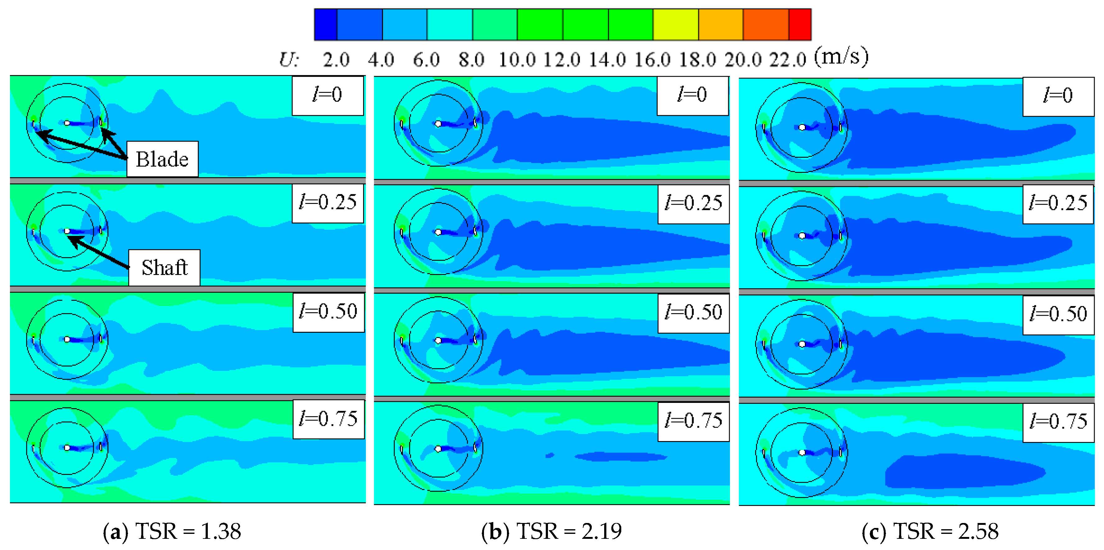
Figure 11.
Fluctuation of wind velocity for the spanwise cross-sections of l = 0, 0.25, 0.50 and 0.75 in downstream region (x/R = 0, 0.5, 1.0, 1.5 and 2.0) at the three different TSRs with the azimuth angle of θ = 90°: (a–e) show the fluctuations of wind velocity of x/R = 0, 0.5 1.0, 1.5 and 2.0, respectively.

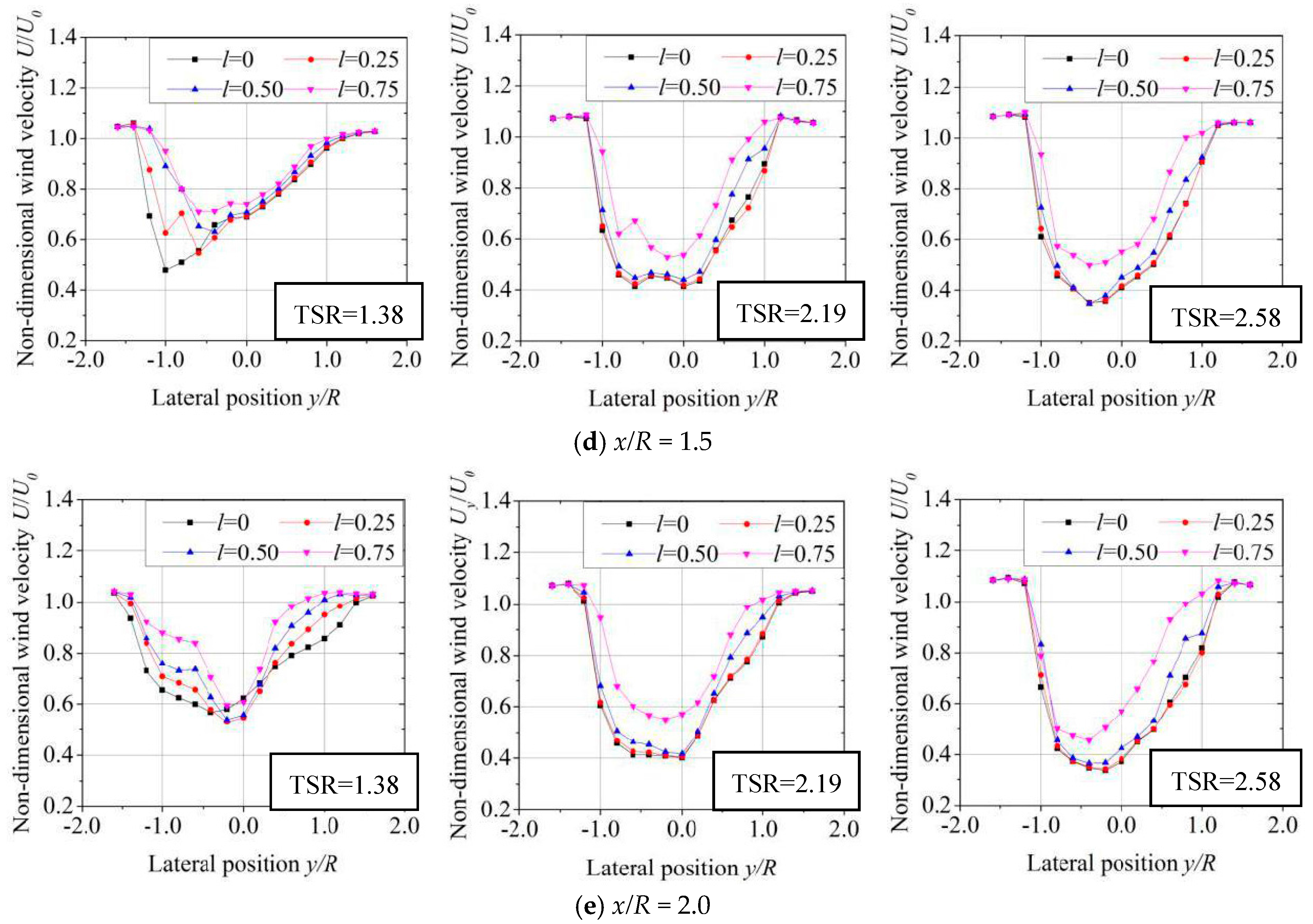
Figure 12.
Comparison of wind velocity deficit between the different spanwise cross-sections of l = 0, 0.25, 0.50 and 0.75 for the downstream region(x/R = 0, 0.5, 1.0, 1.5 and 2.0) at the three different TSRs: (a–d) show the wind velocity deficits of l = 0, 0.25, 0.5 and 0.75, respectively.
Figure 12.
Comparison of wind velocity deficit between the different spanwise cross-sections of l = 0, 0.25, 0.50 and 0.75 for the downstream region(x/R = 0, 0.5, 1.0, 1.5 and 2.0) at the three different TSRs: (a–d) show the wind velocity deficits of l = 0, 0.25, 0.5 and 0.75, respectively.
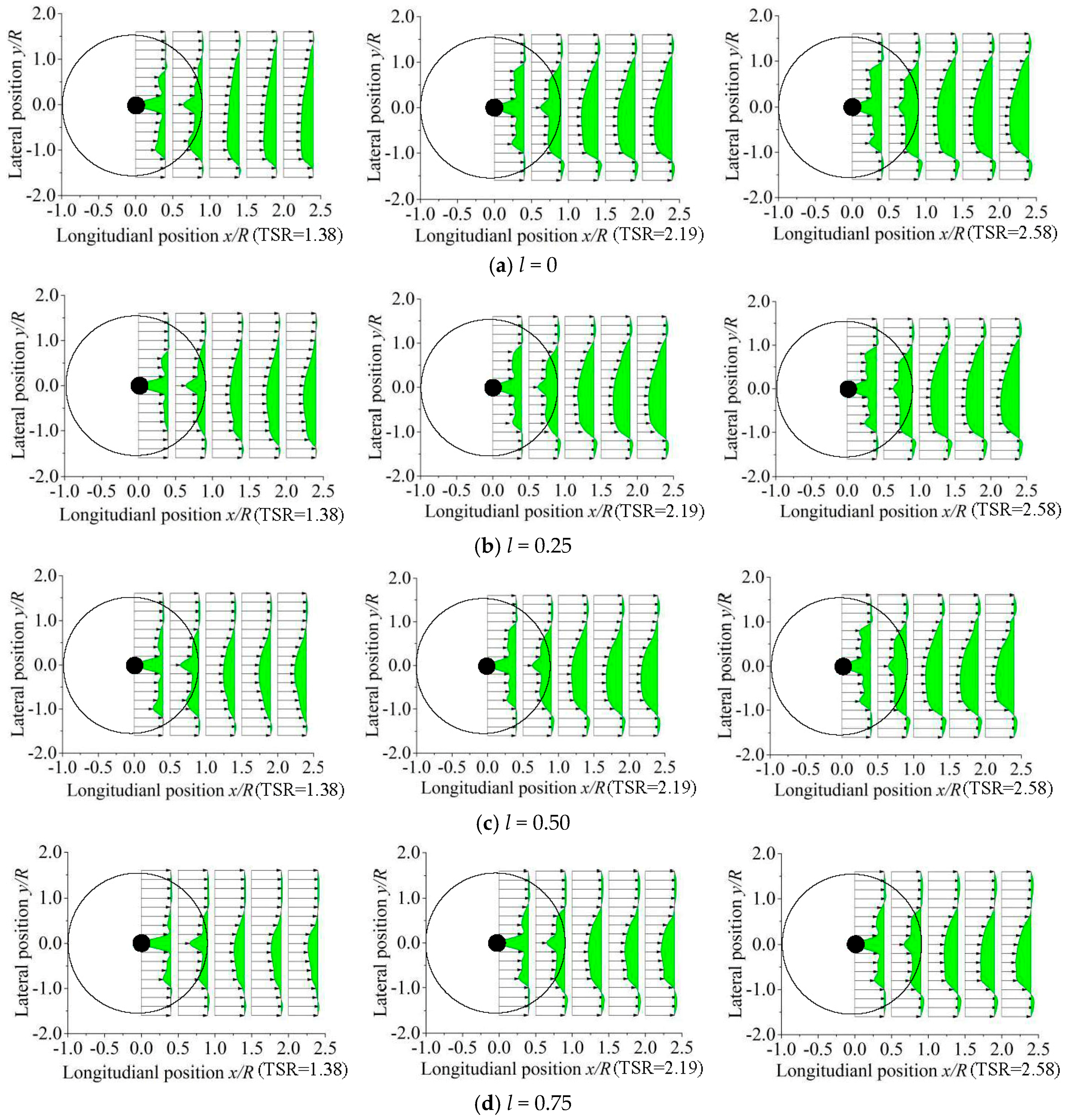
Figure 13.
Fluctuation of torque coefficient in the spanwise cross-sections of l = 0, 0.25, 0.50 and 0.75 for rotor at a rotation period at the three different TSRs (TSRs = 1.38, 2.19 and 2.58): (a–d) show the wind velocity deficits of l = 0, 0.25, 0.5 and 0.75, respectively.
Figure 13.
Fluctuation of torque coefficient in the spanwise cross-sections of l = 0, 0.25, 0.50 and 0.75 for rotor at a rotation period at the three different TSRs (TSRs = 1.38, 2.19 and 2.58): (a–d) show the wind velocity deficits of l = 0, 0.25, 0.5 and 0.75, respectively.

© 2017 by the authors. Licensee MDPI, Basel, Switzerland. This article is an open access article distributed under the terms and conditions of the Creative Commons Attribution (CC BY) license (http://creativecommons.org/licenses/by/4.0/).
Share and Cite
MDPI and ACS Style
Yang, Y.; Guo, Z.; Zhang, Y.; Jinyama, H.; Li, Q. Numerical Investigation of the Tip Vortex of a Straight-Bladed Vertical Axis Wind Turbine with Double-Blades. Energies 2017, 10, 1721. https://doi.org/10.3390/en10111721
AMA Style
Yang Y, Guo Z, Zhang Y, Jinyama H, Li Q. Numerical Investigation of the Tip Vortex of a Straight-Bladed Vertical Axis Wind Turbine with Double-Blades. Energies. 2017; 10(11):1721. https://doi.org/10.3390/en10111721
Chicago/Turabian StyleYang, Yanzhao, Zhiping Guo, Yanfeng Zhang, Ho Jinyama, and Qingan Li. 2017. "Numerical Investigation of the Tip Vortex of a Straight-Bladed Vertical Axis Wind Turbine with Double-Blades" Energies 10, no. 11: 1721. https://doi.org/10.3390/en10111721
Note that from the first issue of 2016, this journal uses article numbers instead of page numbers. See further details here.