
Critical Speed Control for a Fixed Blade Variable Speed Wind Turbine


Division of Electricity, Department of Engineering Sciences, Uppsala University, Box 534, 751 21 Uppsala, Sweden
*
Author to whom correspondence should be addressed.
Energies 2017, 10(11), 1699; https://doi.org/10.3390/en10111699
Submission received: 12 September 2017
/
Accepted: 23 October 2017
/
Published: 25 October 2017
(This article belongs to the Special Issue Wind Generators Modelling and Control)
Abstract
:A critical speed controller for avoiding a certain rotational speed is presented. The controller is useful for variable speed wind turbines with a natural frequency in the operating range. The controller has been simulated, implemented and tested on an open site 12 kW vertical axis wind turbine prototype. The controller is based on an adaptation of the optimum torque control. Two lookup tables and a simple state machine provide the control logic of the controller. The controller requires low computational resources, and no wind speed measurement is needed. The results suggest that the controller is a feasible method for critical speed control. The skipping behavior can be adjusted using only two parameters. While tested on a vertical axis wind turbine, it may be used on any variable speed turbine with the control of generator power.
1. Introduction
For mechanical systems, such as wind turbines, natural frequencies are an important concern. If a system frequency of low damping is excited, it can result in large movements and stress of the mechanical structure. Most modern wind turbines utilize variable rotational speed operation to maximize energy extraction from the wind. While the three-bladed horizontal axis wind turbine is a common sight, the vertical axis wind turbines (VAWTs) are still unusual as commercial energy producers. Since the invention of the lift-based VAWT in the 1920s, several vertical axis concepts have been studied, and the technology is still subject to active research by companies and universities [1,2,3]. Possible benefits are lower maintenance need, low noise and lower center of mass [4]. However, one of the main concerns with the VAWTs is the cyclical aerodynamic forces [5]. Variable pitch VAWTs have been studied, but the cost and reliability issues associated with a pitch mechanism have not yet been solved [2].
For a VAWT with fixed blades and variable speed operation, the oscillating forces are likely to interfere with the mechanical design. If handled properly, a natural frequency excitement in the operational range could be a cost benefit to tolerate. Traditional horizontal axis wind turbines with pitch control can utilize individual blade pitching to damp tower oscillations [6]. Such an option is unavailable for fixed bladed turbines. Another option is to avoid operation at those critical speeds where a natural frequency is excited.
Wind turbine operation can be divided into different regions depending on wind speed:
- Region 1: Below cut in wind speed.
- Region 2: Between cut-in and below nominal wind speed.
- Region 3: Above nominal wind speed.
There is also a point of cut-out where the turbine shuts down. In Region 2, the aim is to maximize energy extraction. The algorithms used are sometimes referred to as maximum power point tracking (MPPT) algorithms [7]. There are several proposed strategies for keeping optimal power output during different wind and weather conditions [7,8]. A well-known strategy is to determine the reference torque as a function of the rotational speed, here on referred to as optimal torque or optimal power control [7,9,10,11]. While this strategy and several other studies focus on operation in Region 2, it should be stated that Region 3 operation also is of interest, especially for fixed bladed turbines [12,13].
In this work, a control handling a critical speed in Region 2 is presented. The controller has the same goal as the torque control with a speed exclusion zone illustrated in [14]. While not providing any details on the design or performance, a PI-controller (proportional-integral controller) is suggested (in [14]) to handle the power reference, and some logic is required to determine switching between set points. A similar controller, which combines a torque controller with a speed controller, is implemented in [15]. Another approach is to use a single continuous torque curve, as summarized in [16]. The implementation has a potentially low complexity, even if the performance is more difficult to control. An example of a potential problem with algorithms using a single curve is that the torque demand at the critical speed is essentially the optimal torque. This delays the transaction and may leave the turbine running at or close to critical speed for some time. The controller presented here achieves the control logic and dynamics using two power reference curves. A state machine keeps track of which curve to use. The dual curve approach allows for more distinct transactions across the critical speed, and the state machine adds a hysteresis to the controller. The idea is similar to “Control System 1” implemented for a 3 MW two-bladed horizontal axis wind turbine in [17]. The work in this paper extends the dual curve designs with a distinct torque demand at the actual critical speed to ensure high avoidance of that operation point. The transaction speed is adjustable using a parameter. Additional parameters are defined to control the skip tendency of the controller. Furthermore, the obtained reference power curves are smooth. This allows for an electric power controller with high bandwidth on the reference value, while limiting shaft vibration excitation.
The design of the power curves and the impact of the parameters are carefully explained and the resulting control can be implemented as lookup tables (LUTs) in a controller unit. The critical speed controller uses the power in the wind to accelerate the turbine, and no active power flow to the generator is provided. Additionally, a feed forward controller is implemented to enable fast generator control, despite the passive rectification and the DC-link.
Operation in Regions 1 and 3 (below cut-in and above rated) is considered beyond the scope of the paper. However, a simplified solution is implemented to allow for experiments, inspired by the considerations expounded in the simulation study [18].
The controller has been implemented and tested on the 12 kW VAWT that was designed and built by the Division of Electricity at Uppsala University, Sweden [4]. The turbine is an H-rotor (straight bladed Darrieus rotor design) with three straight fixed blades (i.e., no pitch mechanism). Its aerodynamic performance and the forces acting on the turbine have been studied in [19,20,21]. The mechanical power is transmitted using a steel shaft directly connected to a permanent magnet synchronous generator (PMSG) placed at ground level. The three-phase generator power is rectified using diodes (AC/DC) and the DC-power is inverted (DC/AC) to three-phase 50 Hz, filtered and dissipated in a resistive load. The use of a long shaft together with a heavy generator rotor can smooth the torque ripple associated with passive rectification [22]. A similar system at a larger scale (200 kW) has been successfully grid connected [23,24].
The controller is an adaptation of the new control and measurement system implemented for the prototype in 2014 [25]. The next section explains the controller in detail. Before the results are presented, the setups for the experiment and simulation are explained.
2. Control and Electrical Design
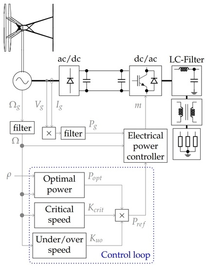
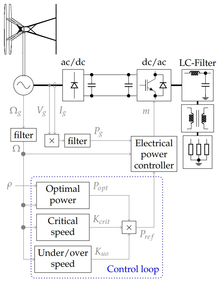
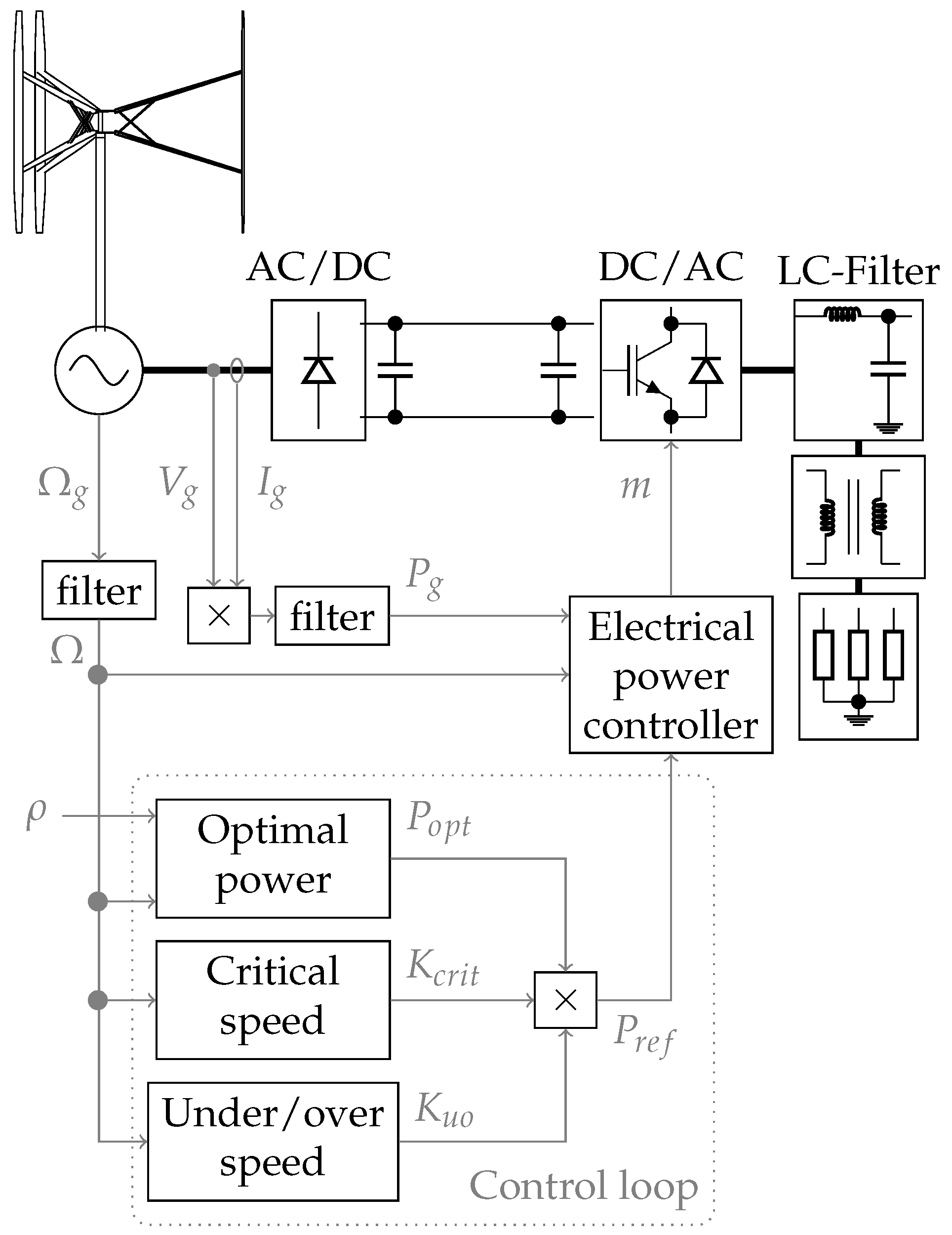
An overview of the control system is illustrated in Figure 1. Each part is described in this section.
2.1. Optimal Power Control in Region 2
A simple, yet effective control strategy in Region 2 (between cut-in and nominal) is based on the concept of estimating the desired torque output depending on the current rotational speed [9]. The strategy can also be expressed as power reference by simply multiplying the torque reference by the rotational speed [11]. The resulting optimal power control strategy is expressed as:
where is the air density, is the turbine radius, A the turbine area, is the maximum power coefficient of the turbine at optimal tip speed ratio and is the rotational speed.
The projected area of an H-rotor is , where H is the blade height. The strategy assumes that and are constant, and all constants can be collected into as:
The air density changes with weather conditions and is better kept outside of [10]. Indirect measurements of can be done using the temperature and the ideal gas law and could be considered a fairly inexpensive measurement to make.
Further improvements can be added to (2). One simple action is to implement a reduction factor in the range 0.8 to 0.99 (1 to 20%). The reduction factor improves the turbine energy capture during turbulent winds. Since the power in the wind changes with the cube of the wind speed, it is more important to follow wind gusts than lulls. The reduction factor keeps the turbine at a higher operational speed, thus improving energy capture at gusts [10].
The efficiency of the mechanical system, the generator and the electrical system up until the electrical power measurement can be considered a function of rotational speed and generator current. The efficiency could be estimated during operation and added to the control as an additional factor. Another option, which is used here, is to consider the losses fairly constant and therefore integrated as a part of the constant reduction factor . The control strategy to obtain the reference power is then:
It is also possible to subtract a compensation factor for the inertia of the system, proportional to the rotational speed derivative, which can improve the response of the turbine [26]; however, we are excluding this option here.
2.2. Critical Speed Controller
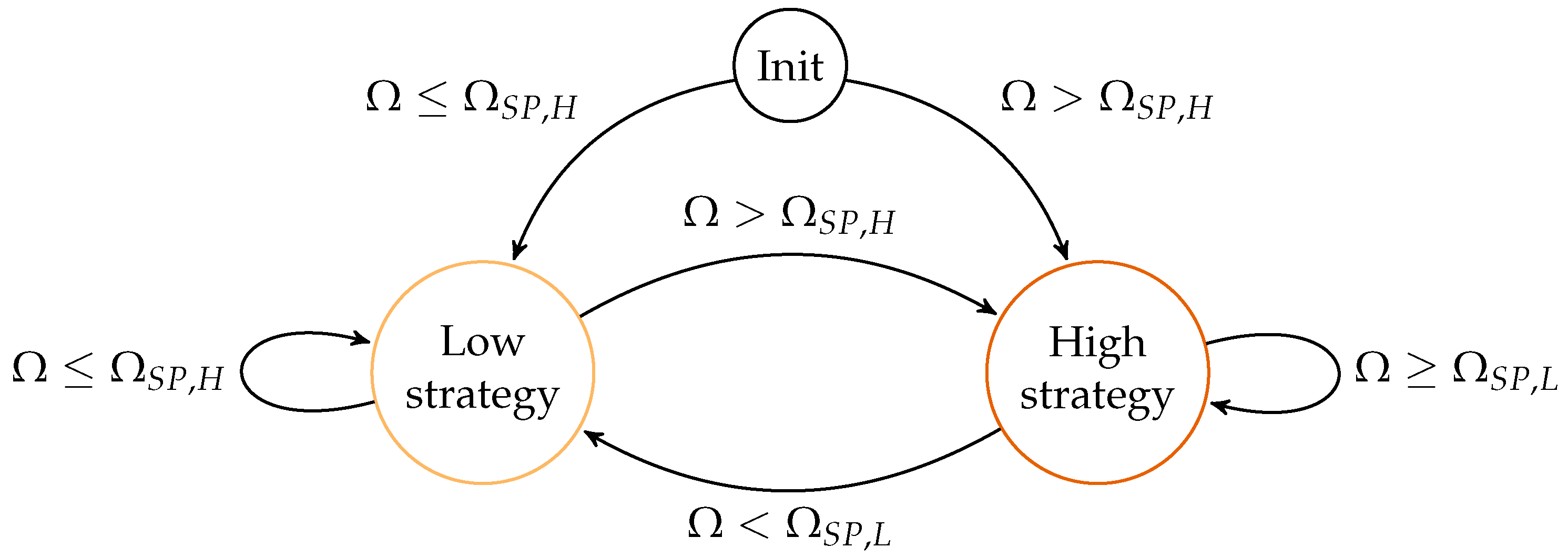
The critical speed controller is based on holding the turbine rotational speed below or above a critical speed region until the wind conditions favor a skip to the opposite side of the region. These thresholds (hold positions) are further on referred to as hold low and hold high and are placed on opposing sides of the critical speed. The presented design achieves the control by adjusting the output power using a relative power output factor, ; see Figure 1. The factor is determined as a function of rotational speed implemented as two LUTs, illustrated in Figure 2. The LUTs are both based on a set of key points, according to Table 1 and Table 2. The points in between the key points are interpolated using a cubic spline algorithm. The resulting LUTs are implemented in the controller. A simple state machine handles switching between the LUTs, depending on current state and rotational speed as (also illustrated in Figure 3):
- “Init”: At system start, “Low” or “High” is selected based on if it is above or below “Switch-point HIGH”.
- The “Low”-strategy is used up until the rotational speed of “Switch-point HIGH”.
- The “High”-strategy is used down to the rotational speed of “Switch-point LOW”.
The state machine and the switch points provide a hysteresis to the controller. The key points and the controller parameters are further explained in the following sections. Moreover, Table 2 includes a guide for the selection of the different parameters. This short guide aims to simplify for the designers to optimize the parameters for their operation conditions. The presented points, their values and the chosen design parameters are the result of an iterative design process with simulations of different cases. The goals of this manual optimization process were to have good avoidance of the critical speed, high power extraction, reasonable time between transactions and to limit the amount of tuning parameters.
2.2.1. Hold Low, Hold High
As soon as the hold point is passed, the turbine should find a new operating point close to optimal speed and power beyond the critical speed. This can be achieved by a match in the relative power, , at the hold point to the relative power at the end of the skip. The equations to determine the relative power at the two hold points are derived in Appendix A.
To allow for adjustment of the switching behavior, two parameters are introduced: hold low coefficient, , and hold high coefficient, . To increase the skip tendency of the controller, the can be lowered and increased. The opposite makes the controller less likely to skip.
2.2.2. Switch-Point Low, Switch-Point High
The switch-points are the points where the state machine will switch state and LUT to use. The switch-points are placed before the hold points are reached, to achieve the hysteresis effect after a skip has been performed. The placement is also close to the hold points to achieve a quick switch after a completed skip. The relative power for the high and low strategy curves (LUTs) must have the same relative power at each switch-point to allow for a smooth switch.
2.2.3. Critical
The relative power at critical speed, , is adjustable with parameter . The transaction is faster with higher values of . The low strategy uses a lowering of relative power to allow the turbine to spin up. The high strategy increases relative power at critical speed to slow down the turbine. It is preferable to keep positive torque from the generator at all times to avoid leaving the two-mass system without any damping. Maximum output power of the electrical system and torque stress of the driveline must also be considered. These demands put limits on the maximum value of .
2.2.4. Controller Limitation
An important limitation for the skip range of the controller is the wind speed turbulence. If the desired range to avoid is too wide, the turbulence in the wind can result in failed skips. This was observed during the development of the controller curve shape. Failed skips are a problem if the critical position is passed without reaching the switch-point, followed by a large change in wind speed, keeping the turbine at the critical point, held by the slope at the critical point. The proposed controller minimizes this risk by locating the switch-points close to the hold points. Since the power at the hold points is defined by the power at the opposite side of the skip, the wind change must be very significant to prevent the skip from being completed. One possible solution to handle the risk of failed skips is to add a state to the state machine that is entered when the critical speed is crossed. The new state counts time samples and forces a state-change if a switch-point has not been reached within a certain time-out. The current setup showed no tendency for failed skips; therefore, such a solution has not been implemented here.
Another limitation to consider is if the critical speed is close to the cut-in or cut-out wind speed. It may still be possible to use the general idea, but the presented design will need consideration.
A requirement for the controller to work is that should be somewhat constant over the skip range. The requirement is needed for the hold positions to work. If drops more than the power in the wind changes between the hold point and the end of the skip, there will be no hold. Instead, the hold low peak (or hold dip for the hold high) would be insignificant or even inverted. Due to the power in the wind changes with the cube of the wind speed, this requirement is probably fulfilled by most turbines.
2.3. Under-/Over-Speed Control
This work focuses on operation in Region 2 (between cut-in and nominal). However, to perform the experiments, an under-/over-rotational speed control had to be implemented.
For the current setup, and reasonably for most turbine systems, some losses are more prominent at low power levels (in relative terms). Such losses are iron losses in the generator, mechanical losses and transformer magnetization losses. Additionally, the power coefficient , which mainly depends on the tip speed ratio, also decreases slightly at lower wind speeds. Because of these issues, the turbine can stop, or react slowly when controlled by the (3) strategy at low wind speeds [18]. Therefore, an under speed control was implemented inspired by the work in [18]. The same approach was chosen for the over speed limit giving rise to the under-/over-speed controller as follows:
where is the generator rotational speed in . Note that the over-speed control is a rough solution to allow for the experiments and should not be considered a suitable method for effective control in Region 3.
2.4. Electrical Power Controller
The control system provides a reference power as input to a power controller. The power controller adjusts the modulation level of the DC/AC-inverter to ensure that the reference power is drawn from the generator. The load in this setup is a fixed resistive load, and the output power is therefore proportional to the square of the product of the modulation level of the inverter and the DC-link voltage. Furthermore, the DC-link voltage for a diode rectified permanent magnet synchronous generator can be approximated as proportional to the rotational speed [27]. By ignoring the dynamics of the DC-link capacitors and system efficiency, the output power can be approximated as the generator power. The generator power can then be expressed as:
where m is the modulation level of the converter and is a feedforward coefficient, here chosen to be in the denominator. Since the desired generator power is the reference power for the controller, the modulation level can be determined by solving (5) for m and replacing by the reference power . The static error is reduced by adding an integration of the feedback error. The complete controller can be described as:
where is the integration part coefficient, and it was determined during experiments. The feedforward part provides knowledge to the controller about the disturbance . An initial guess of the constant can be determined from system data and then fine-tuned during tests. It can be noted that it would have been possible to use a measurement of the DC-link voltage for the feedforward part instead. Since the presented approach has a low number of measurements and worked well enough, this option was not explored. The integration part of the real sampled system was implemented as a sum, and conditional anti-windup was used. The conditional anti-windup has acceptable performance, low complexity and requires no additional parameters [28].
2.5. Rotational Speed Filter
Any noise or high frequency oscillations on the rotational speed measurement will strongly impact the power reference according to (3). Therefore, filtering of the rotational speed measurement is reasonable. Here, a digital low pass filter was implemented as a moving average filter, sampled in synchronization with the rotational speed. Previous measurements indicate the propagation of aerodynamic torque ripple for this prototype to be surprisingly low [21]. Even so, the rotational speed synchronized filter cutoff was chosen below once per revolution to avoid any aerodynamic ripples to disturb the control system. The chosen approach also puts the filter cutoff well below the expected natural frequency of the shaft for all operational speeds. Another solution, if higher bandwidth had been required, could have been a notch filter, as suggested in [29].
2.6. Generator Power Filter
For the generator power filter, the main concern is the electric power ripple due to the passive rectification. The ripple has been shown to have limited mechanical impact on the prototype system [22]. However, the ripple would disturb the controller. A digital Butterworth low pass filter was implemented as the generator power filter.
3. Experiments
3.1. The Prototype
The experiments were performed on the 12 kW VAWT built by Uppsala University. The open site turbine is located at the Marsta Meteorological Observatory close to Uppsala, Sweden. The generator three-phase output is passively rectified using a six-pulse diode bridge. The DC-voltage is inverted into three-phase AC-voltage with 50 Hz by an SPWM-inverter (sinusoidal pulse width modulation). The inverter is of in-house design, based on three SEMIKRON SEMiX252GB126HD IGBT-modules (Insulated-Gate Bipolar Transistor). The IGBT drivers are SEMIKRON Skyper 32 PRO with evaluation boards (SEMIKRON INTERNATIONAL GmbH, Nuremberg, Germany). The AC-power is filtered and transformed before being dissipated in a Y-connected resistive load.
The properties of the prototype system are listed in Table 3. The output currents, voltages and rotational speed of the generator are measured. During the experiments, a force measurement system was attached to one of the turbine blades giving the tangential blade force and the normal blade force . The sampling of electric power and forces is synchronized in the software. The control and measurement system was programmed in NI LabVIEW™ software (National Instruments, Austin, TX, USA). The system is described in detail in [25]. The control system was redesigned to implement the controllers described in Section 2, resulting in the system illustrated in Figure 1.
3.2. Measurement Campaign and Data Treatment
The operation of the prototype was limited to 4 kW and 90 rpm due to the force measurement setup [25]. The turbine system is not expected to have any natural frequency in the range 40 rpm to 90 rpm, and therefore, virtual critical speeds were selected. The method of using fictive critical speeds can also be considered a safer method for controller evaluation. Two critical speeds were selected: 55 rpm and 75 rpm. Weather conditions matching optimal rotational speed close to the critical speed were awaited. Two good measurement series, one for each critical speed, were obtained in this matter on 2 and 5 July 2017. The lengths of the measurements were 60 min and 12 min, respectively.
The control system uses an overall sample rate of 2 kHz. The wind speed was sampled at 1 Hz. The rotational speed and generator electric power were averaged over 1 s. The force measurements were kept at 2 kHz and calibrated based on periods of low wind speeds [25].
4. Simulations
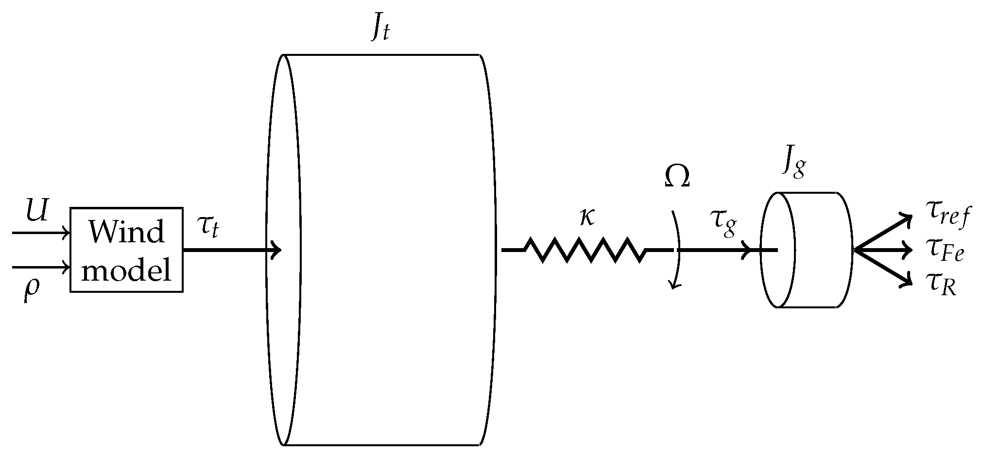
The simulations were performed in MATLAB Simulink (MathWorks Inc., Natick, MA, USA) as transient simulations using one-dimensional rotating components. The model is illustrated in Figure 4, and the model parts are further described in this section. The simulations were a vital tool in the design process of the controller. The verified simulation model also provided a simple way to evaluate the performance of the controller by comparing simulations with and without the controller active. Since site conditions were fluctuating, it was difficult to make such evaluation processes with on-site experiments.
4.1. Wind Model
A low complexity aerodynamic model to provide the torque from the wind was used:
where U is the wind speed, and the power coefficient curve, , was based on previous measurements on the prototype [19]. A piecewise cubic polynomial was fitted to the measurement and implemented as a function block in the simulation.
4.2. Load Model
The model of the generator, diodes, DC-link, DC-link capacitors, inverter, filters, three phase load and power controller were all reduced to an ideal mechanical torque source according to:
The reduction of the load can be motivated by the power controller described in Section 2.1. The controller targets maintaining a constant power from the generator, and the dynamics of the diodes and the power control system are in much shorter time frames than studied here. The reduced model allows for much faster simulations compared to a full electric circuit simulation with diodes.
The iron losses were set as a linear function of the rotational speed based on a curve fit to measurements done on the generator [30] resulting in:
which was implemented as a rotational damper on the generator shaft.
The generator voltage of a PMSG can be approximated as:
where is the voltage constant of the generator. The generator current can then be derived as:
The braking torque by the resistive losses could then be approximated as:
which was calculated and implemented as an ideal braking torque on the generator shaft.
4.3. Model of the Power Controller with Critical Speed
This section describes the three blocks of the control loop and the implementation of filters for simulating the system illustrated in Figure 1. The rotational speed was filtered using a low pass filter implemented as a transfer function with a cutoff at 1 Hz. This simplification gives the filter the same cutoff as the real filter at about 70 rpm. The rotational speed signal was then sampled at a fixed sample rate by a zero-order hold block. The discrete signal simulates the controller loop in the control system.
The output ideal torque was the product of the following three blocks:
- Optimal power: This block was using the filtered rotational speed together with the power from (3) to obtain the torque reference.
- Critical speed control: This block contains the state machine and the two LUTs of relative power for the low and high strategy. The LUTs, with a resolution of rad/s, were implemented in a function block. The state was fed back to the next iteration using a delay-block.
- Under-/over-speed control: This block was using the filtered input rotational speed together with (4) to obtain the relative torque output.
4.4. Tower Model
A tower model was introduced to obtain an intuitive measure of the potential movement of a system with a natural frequency in the operating range. Due to three-blade symmetry, most of the non 3 p-multiple components in the aerodynamic forces are expected to be cancelled out, as shown for the tangential force in [21]. Of the remaining frequencies, the 3 p component is assumed to dominate. Hence, the oscillating part of the aerodynamic forces acting on the tower can be modeled as:
where a is a constant that was selected to obtain a reasonable size of the tower movement when not operating in the critical range.
The fictive tower was modeled as a damped spring-mass system. The mass was selected close to the prototype turbine mass, and the damping was set low to achieve an underdamped system. The resulting transfer function returning the position of the tower was implemented in Simulink as:
where k is the spring constant of the tower, which was adjusted to achieve a natural frequency at the desired point. The function was evaluated in the time domain and fed as input to the transfer function. Two different towers tuned to two critical speeds were simulated. The frequency response of (14) for the two towers is plotted in Figure 5.
4.5. Validation of the Simulation Model
The simulation model was compared with the two measurements time series, which were obtained as explained in Section 3.2. The hold coefficients for the critical controller, and , were fine-tuned until similar performance in terms of skip tendency could be observed.
4.6. Evaluation of the Critical Speed Controller
The simulation model was used as a tool for evaluating the controller performance. The rotational over-speed control was disabled during the evaluation simulations to isolate the behavior of the critical controller. A real wind speed time series of 3600 s from site measurements was selected. The time series was adjusted by adding an offset chosen to force the average (AVG) wind speed to match two different specific optimal rotational speeds. The critical speed for the system was then set to the same rotational speed. This approach provided a stress test of the system, since the optimal speed would be around the critical speed. Real winds have a more complicated behavior; however, the chosen approach should be useful for evaluation purposes. Two more simulations were performed with the wind speed offset value optimized for the cubic mean cube (CMC) instead of the average. Since the power in the wind increases by the cube of the wind speed, these tests could potentially stress the system even more [31].
For each of the four simulation setups, a reference simulation was performed. During the reference simulation, the critical speed controller was disabled (), leaving the turbine operating at optimal power control. The simulations were evaluated with respect to the corresponding reference simulation. The evaluation parameters were selected as:
- Number of skips (transactions) across the critical speed (up or down).
- Energy capture.
- Time spent within rpm of the critical speed; see Figure 5.
- The MAD (mean absolute deviation) of the power fluctuation.
- The expected tower dimension based on fatigue due to the movement at critical speed.
- Maximum shaft torque.
Evaluation parameters 2–6 were expressed as (%) with the critical speed controller relative to the critical speed controller disabled. The methodology of 5 is described in detail in the following section.
4.6.1. Tower Fatigue Estimations
The fictive tower model used here represents a very fast system, i.e., the controller cannot skip the critical speed fast enough without exciting the tower to maximum movement amplitude. A real tower with such properties would need to be designed to handle the full movement range, even with the critical speed controller implemented. However, there are still potential gains of using the controller, when considering fatigue. The material under stress, caused by the tower movement, is assumed to have an SN-curve (Wöhler stress cycle curve) modeled by:
where is the stress, the ultimate stress before failure and N the number of cycles. The parameter B is a material property. The tower movement is assumed proportional to the stress , and the movement required for failure is assumed proportional to . The stress cycles are analyzed using the rainflow method with 100 stress bins. The total damage can then be calculated using Miner’s rule as:
where M is the number of bins (here ), is the number of cycles for bin i and is the number of cycles to reach failure for the stress amplitude at i. The design criteria for the tower was chosen to be 20 years of continuous operation with the critical wind time series. The required tower strength according to the calculations was used as the result.
This work uses the tower as a reference. However, the fractional nature of (15) makes the statements valid for the strength of any part in the turbine system that is subject to stress that is linear to the tower movement. The weakest expected material in the wind turbine should be close to glass fiber with .
4.6.2. Driveline Endurance Limit
Depending on the turbine design, it may be reasonable to design the critical driveline components so that nominal torque oscillations are within the endurance limit. It may even be a side effect of other requirements. For instance, the design criterion for the studied concept is a short-circuit event in the generator. Accounting for the safety margin, the design torque for the shaft should be in the range of 5–10 times the nominal torque. A steel shaft has an endurance limit at about 20% of the designed break limit [32]. Hence, the nominal torque should be within the shaft endurance limit.
4.6.3. Parameter Study of the Critical Coefficient
The impact of the critical coefficient, (see Table 1 and Table 2), was studied through simulations for a set of values of between 0.2 and 0.8. The same wind time series was used as in the evaluation and adjusted to force the average (AVG) wind speed to match two specific critical rotational speeds. The study illustrates the trade-off between fast transactions and increased maximum shaft torque.
5. Results and Discussion
5.1. Experiments
Measurements from the test runs with a fictive critical speed at 55 rpm are presented in Figure 6. As can be seen by the rotational speed, the controller quickly passes the forbidden region both when moving up and down in rotational speed. Given the rather unsteady wind, the controller is still limiting the number of skips. A seemingly quick skip up and down is noticed at 800 s, and the period lasted about 80 s. Similarly, a skip down and up is observed at 1300 s, and this period lasted about 30 s. Given the size of the turbine prototype, these could be considered acceptable time scales for skipping.
There are significant power fluctuations during operation. The skips are expected to give rise to fluctuations. During operation close to the critical speed, the power fluctuations increase. This is especially clear in the 75 rpm case; see Figure 7. In the region above 600 s, the rotational speed is close to constant; however, the power is still fluctuating similarly as during the skips in the period 300 s to 600 s. The main reason for this is likely the over-speed control keeping the rotational speed down during the turbulent wind, giving rise to power surges.
The measured forces mainly show a correlation with the operating point, which is expected due to the increased flow velocities. No distinct effects are shown from the skips themselves. Note however that no real natural frequencies are passed through during the skips. The measured tangential force is affected by turbine dynamics, and shaft-induced torque may be difficult to observe [25].
5.2. Validation of the Simulation Model
The resulting values for the hold coefficients are and ; see Table 2. The resulting simulation based on the same wind vector as measured during the experiments is shown in Figure 6 and Figure 7. After adjustment of and , the model compares well with the experiments. Some skips can happen at different positions, but the total number of skips is about the same for both the 55 rpm and 75 rpm cases.
During the tuning of and , it was clear that the simulated model was more responsive and performed skips more frequently than the real measurements. The reason for this is likely correlated to the wind speed. On site, the wind is measured at one small point using a fast acoustic wind meter. In the model, this measured wind is extrapolated to be the wind over the full active turbine volume at an instant.
5.3. Evaluation of the Critical Speed Controller
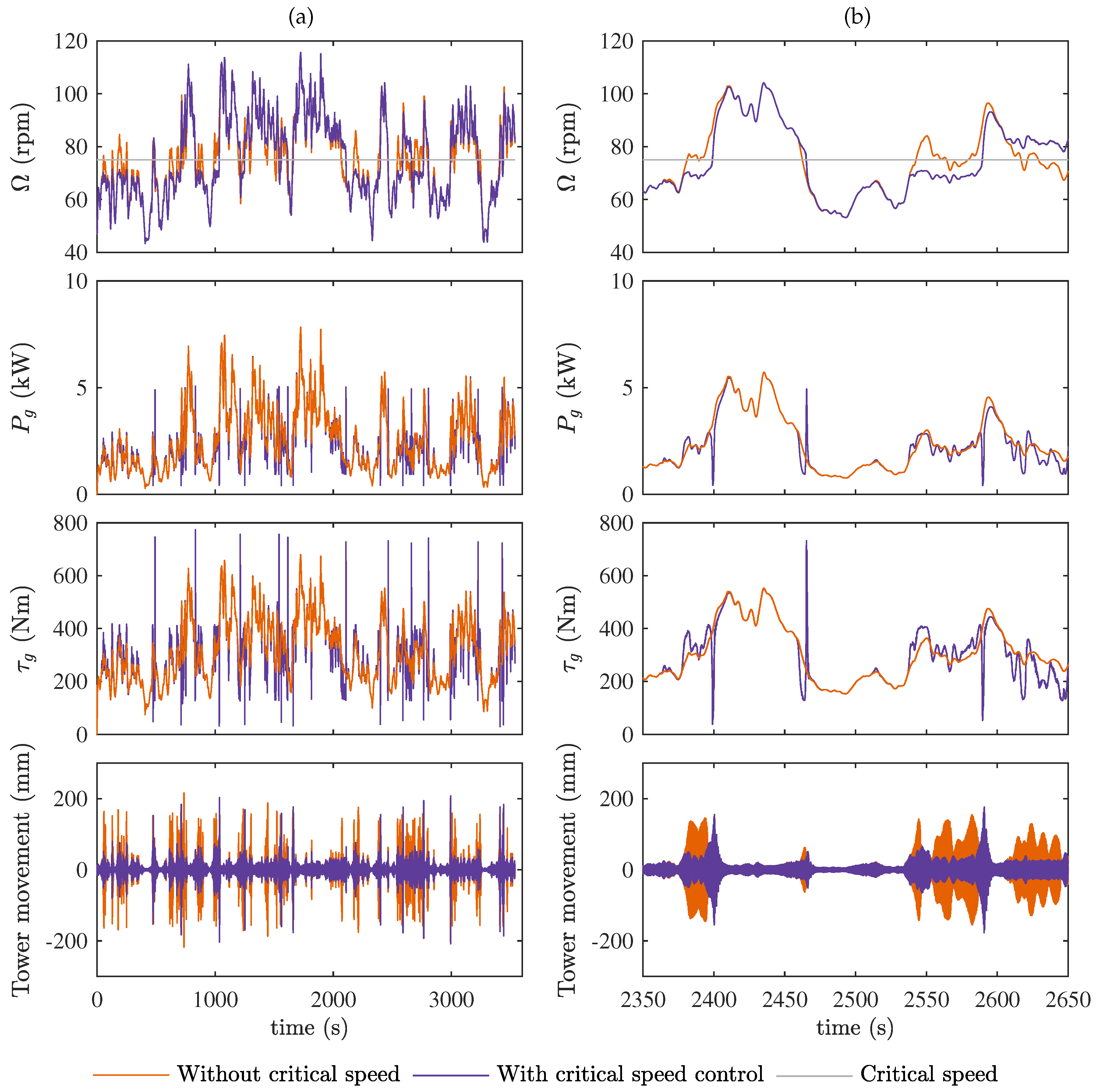
The performance of the critical speed controller is summarized in Table 4, and the time series from the 75 rpm AVG case is illustrated in Figure 8. The time series for the 55 rpm case and the CMC cases have a similar appearance. For the studied cases analyzed for 3600 s, the optimal torque control spends a total time of 410 to 480 s within the critical range. That is surprisingly low, considering that the wind speed time series has been selected and adjusted to maximize operation at the critical speed. The turbulence in the wind together with optimum torque control is continuously changing the rotational speed. The critical speed controller is still able to reduce the time within the critical range by more than 90%. The penalty in terms of energy capture is 2% for the higher rotational speed cases and almost 10% for the 55 rpm cases. The controller skips on average about every 230 s in the 55 rpm case and almost twice as often for the 75 rpm case. This likely explains the higher energy capture for the 75 rpm cases, since the turbine skips faster to a more optimal rotational speed. The reason for the more frequent skipping in the 75 rpm case is likely due to increased turbulence power at the elevated average speed (since the power in the wind scales with the wind speed cube).
The amount of overall movement of the fictive tower is reduced allowing a possible reduction of tower dimensioning of about 25%. The control is unable to remove the peaks entirely. The duration of the peaks is clearly reduced, but the low response time of the tower model makes it quickly reach the peak amplitudes.
The power fluctuations in the generator decrease by around 9% for the 55 rpm cases and increase with 4% for the 75 rpm cases; see also Figure 8. It is remarkable that the overall power fluctuations are lower or only slightly increased with the controller action. Clearly, the turbulent wind itself is the main source of power oscillations. There are narrow peaks and dips in the power and mechanical torque at the actual skips, unrepresented when the controller is disabled; see Figure 8b. The peak torque is below nominal torque in all cases, but it is close to nominal for skip down. The skips perform a cycling of the torque that can be more stressful than oscillations during normal operation. However, for drivelines designed with an endurance limit above nominal torque, this should not be a problem.
The results from the parameter sweep of the critical coefficient, , that impacts the power peaks at critical speed are presented in Table 5. The parameter value seems to have a limited impact on the results. None of the cases resulted in a failed skip. For the 55 rpm cases, it seems that a low is beneficial for both the tower and the shaft. Otherwise, an improvement in maximum shaft torque can be noticed at lower values of , while the tower needs to be stronger, as expected.
5.4. General Discussion
While the controller aims to keep the tower natural frequency at bay, the two-mass system described in Figure 4 has a natural frequency of its own. During the simulations, it was clear that too aggressive changes in reference power could trigger the rotor mass to have some oscillation. Therefore, spline interpolation was selected to achieve smooth curve shapes. The smooth transactions keep the natural frequency of the shaft unexcited. The control loop speed in the simulations had to be higher than in the experiments to keep stability. Possible reasons for the difference could be the different filters topologies between the experiments and the simulations and some damping in the system not covered by the simulations.
There were some power fluctuations observed in the measurements (Section 5.1) that seemed possibly caused by the controller itself. According to the simulations, the power fluctuations with the critical speed controller are similar to those when operating at optimal torque. This contradiction could in part possibly be explained by the aggressiveness of the simulations compared to the experiment (as discussed above). An additional explanation could be that the over-speed controller is activated to keep the rotational speed down. Furthermore, it can simply be an effect of the increased energy of the turbulence at higher wind speed, which causes the higher power oscillations.
The tower movement at critical speed for the fictive tower studied here is significantly higher than at other operation points within Region 2. Therefore, fatigue benefits can be obtained by implementing this controller. For a tower of greater damping at the critical speed, the movement may be less than for normal operation at higher wind speeds. In that case, the tower must still handle continuous movement of that amplitude. However, if that operational case is uncommon, while operation close to the natural frequency is common, there could be fatigue benefits to implement a controller to limit the time at the natural frequency.
6. Conclusions
The presented critical speed controller was shown to be a feasible method to skip a critical speed related to a natural frequency. The experimental runs at two fictive critical speeds show that the controller works as intended. There were no real critical speeds in the operational range; however, the measured forces showed no indication of added stress due to the skips performed by the critical speed controller. While the presented concept was tested on an H-rotor vertical axis turbine, it should be possible to implement it on most wind turbines with the control of active power flow from the turbine. There is a theoretical risk that some failed skips could lead to operation close to the critical speed. This could be an issue with very light turbines operating at highly turbulent winds. The prototype showed no indication of such problems; still, a possible solution to handle the risk has been suggested.
The simulations show that the controller can reduce the time spent close to a critical speed by more than 90%. The overall tower movement is reduced by 30%, with similar peak amplitudes. This has the potential to lower the fatigue of the tower. The controller adds stress to the driveline (shaft) and electrical system; however, the peaks are still within nominal range. There is an energy capturing loss, which is a trade-off with the skipping tendency. The skipping tendency is dependent on the energy in the wind speed turbulence. Most design parameters are fixed, and tuning of the skipping tendency can easily be adjusted using only two parameters. The overall power fluctuations caused by the controller appear to be similar to those detected when the turbine is running with the optimal torque control. However, short duration peaks and dips are introduced at the actual skips that need consideration.
The presented system requires few measurements and little computational resources to be implemented; however, knowledge of the turbine power coefficient curve is required. The control uses only the power in the wind for accelerating, allowing for diode rectification and ensuring torque direction to be the same through the skip. Compared to similar methods, the presented controller requires little resources for operation and is relatively easy to implement, at least compared to the functionality provided. The controller provides a smooth reference power, which can be beneficial for the actual power controller design. The speed exclusion zone and the transaction aggressiveness together with the tendency to skip can all be easily adjusted. While the presented controller can handle operations close to cut-in, the region above nominal has not been addressed.
A final observation is that the wind speed turbulence continuously changes the rotational speed. It may therefore be unlikely for a turbine to be stuck at a critical speed for a long time. Depending on the site turbulence conditions and the responsiveness of the turbine, this could allow for an alternative control approach, where vibration monitoring assists the power controller. Furthermore, it should be stated that these types of controls are essentially a trade-off between loss of energy production and material cost.
Acknowledgments
The J. Gust Richert foundation is acknowledged for contributions of equipment for the experiments. This work was conducted within the STandUp for Energy strategic research framework, and it is a part of STandUp for Wind.
Author Contributions
Morgan Rossander has done the majority of the work in this paper. Anders Goude participated in the experiments. All authors have taken part in data analysis and interpretation. Sandra Eriksson supervised the project.
Conflicts of Interest
The authors declare no conflict of interest.
Appendix A. Power at Hold Positions
The power at the hold position, , and after the skip is complete, , is:
respectively, where U is the wind speed, which is the same for the two cases. The tip speed ratios are:
where is the rotational speed at the hold position and the rotational speed after the skip is complete. The operation after the skip is complete is aimed to be at the optimal tip speed ratio. Solving (A4) for U and inserting it into (A3) gives:
Expressed relative to optimal operation at :
The obtained expression is valid for determining both the hold low and the hold high relative power for the critical speed controller.
References
- Darrieus, G.J.M. Turbine Having Its Rotating Shaft Transverse to the Flow of the Current. U.S. Patent 1,835,018, 8 December 1931. [Google Scholar]
- Tjiu, W.; Marnoto, T.; Mat, S.; Ruslan, M.H.; Sopian, K. Darrieus vertical axis wind turbine for power generation I: Assessment of Darrieus VAWT configurations. Renew. Energy 2015, 75, 50–67. [Google Scholar] [CrossRef]
- Tjiu, W.; Marnoto, T.; Mat, S.; Ruslan, M.H.; Sopian, K. Darrieus vertical axis wind turbine for power generation II: Challenges in HAWT and the opportunity of multi-megawatt Darrieus VAWT development. Renew. Energy 2015, 75, 560–571. [Google Scholar] [CrossRef]
- Apelfröjd, S.; Eriksson, S.; Bernhoff, H. A Review of Research on Large Scale Modern Vertical Axis Wind Turbines at Uppsala University. Energies 2016, 9, 570. [Google Scholar] [CrossRef]
- Sutherland, H.J.; Berg, D.E.; Ashwill, T.D. A Retrospective of VAWT Technology; Technical Report SAND2012-0304; Sandia National Laboratories: Albuquerque, NM, USA, 2012. [Google Scholar]
- Bossanyi, E.A. Individual Blade Pitch Control for Load Reduction. Wind Energy 2003, 6, 119–128. [Google Scholar] [CrossRef]
- Abdullah, M.A.; Yatim, A.H.M.; Tan, C.W.; Saidur, R. A review of maximum power point tracking algorithms for wind energy systems. Renew. Sustain. Energy Rev. 2012, 16, 3220–3227. [Google Scholar] [CrossRef]
- Musunuri, S.; Ginn, H.L. Comprehensive review of wind energy maximum power extraction algorithms. In Proceedings of the 2011 IEEE Power and Energy Society General Meeting, Detroit, MI, USA, 24–29 July 2011; pp. 1–8. [Google Scholar]
- Novak, P.; Ekelund, T.; Jovik, I.; Schmidtbauer, B. Modeling and control of variable-speed wind-turbine drive-system dynamics. IEEE Control Syst. 1995, 15, 28–38. [Google Scholar] [CrossRef]
- Johnson, K.E.; Fingersh, L.J.; Balas, M.J.; Pao, L.Y. Methods for increasing Region 2 power capture on a variable-speed wind turbine. J. Sol. Energy Eng. 2004, 126, 1092. [Google Scholar] [CrossRef]
- Muljadi, E.; Pierce, K.; Migliore, P. Soft-stall control for variable-speed stall-regulated wind turbines. J. Wind Eng. Ind. Aerodyn. 2000, 85, 277–291. [Google Scholar] [CrossRef]
- Dalala, Z.M.; Zahid, Z.U.; Lai, J.S. New Overall Control Strategy for Small-Scale WECS in MPPT and Stall Regions With Mode Transfer Control. IEEE Trans. Energy Convers. 2013, 28, 1082–1092. [Google Scholar] [CrossRef]
- Andriollo, M.; Bortoli, M.D.; Martinelli, G.; Morini, A.; Tortella, A. Control strategies for a VAWT driven PM synchronous generator. In Proceedings of the 2008 International Symposium on Power Electronics, Electrical Drives, Automation and Motion, Ischia, Italy, 11–13 June 2008; pp. 804–809. [Google Scholar]
- Bossanyi, E.A. The Design of closed loop controllers for wind turbines. Wind Energy 2000, 3, 149–163. [Google Scholar] [CrossRef]
- Licari, J.; Ekanayake, J.B.; Jenkins, N. Investigation of a Speed Exclusion Zone to Prevent Tower Resonance in Variable-Speed Wind Turbines. IEEE Trans. Sustain. Energy 2013, 4, 977–984. [Google Scholar] [CrossRef]
- Schaak, P.; Corten, G.; van der Hooft, E. Crossing Resonance Rotor Speeds of Wind Turbines; Technical Report; Energy Research Centre of the Netherlands: Petten, The Netherlands, 2003. [Google Scholar]
- Yang, J.; Song, D.; Dong, M.; Chen, S.; Zou, L.; Guerrero, J.M. Comparative studies on control systems for a two-blade variable-speed wind turbine with a speed exclusion zone. Energy 2016, 109, 294–309. [Google Scholar] [CrossRef]
- Goude, A.; Bülow, F. Robust VAWT control system evaluation by coupled aerodynamic and electrical simulations. Renew. Energy 2013, 59, 193–201. [Google Scholar] [CrossRef]
- Kjellin, J.; Bülow, F.; Eriksson, S.; Deglaire, P. Power coefficient measurement on a 12 kW straight bladed vertical axis wind turbine. Renew. Energy 2011, 36, 3050–3053. [Google Scholar] [CrossRef]
- Dyachuk, E.; Rossander, M.; Goude, A.; Bernhoff, H. Measurements of the Aerodynamic Normal Forces on a 12-kW Straight-Bladed Vertical Axis Wind Turbine. Energies 2015, 8, 8482–8496. [Google Scholar] [CrossRef]
- Rossander, M.; Goude, A.; Bernhoff, H.; Eriksson, S. Frequency analysis of tangential force measurements on a vertical axis wind turbine. J. Phys. Conf. Ser. 2016, 753, 042016. [Google Scholar] [CrossRef]
- Rossander, M.; Goude, A.; Eriksson, S. Mechanical Torque Ripple From a Passive Diode Rectifier in a 12 kW Vertical Axis Wind Turbine. IEEE Trans. Energy Convers. 2017, 32, 164–171. [Google Scholar] [CrossRef]
- Eriksson, S.; Kjellin, J.; Bernhoff, H. Tip speed ratio control of a 200 kW VAWT with synchronous generator and variable DC voltage. Energy Sci. Eng. 2013, 1, 135–143. [Google Scholar] [CrossRef]
- Kjellin, J.; Eriksson, S.; Bernhoff, H. Electric Control Substituting Pitch Control for Large Wind Turbines. J. Wind Energy 2013, 2013, 1–4. [Google Scholar] [CrossRef]
- Rossander, M.; Dyachuk, E.; Apelfröjd, S.; Trolin, K.; Goude, A.; Bernhoff, H.; Eriksson, S. Evaluation of a Blade Force Measurement System for a Vertical Axis Wind Turbine Using Load Cells. Energies 2015, 8, 5973–5996. [Google Scholar] [CrossRef]
- Bossanyi, E.A. Wind Turbine Control for Load Reduction. Wind Energy 2003, 6, 229–244. [Google Scholar] [CrossRef]
- Knight, A.M.; Peters, G.E. Simple Wind Energy Controller for an Expanded Operating Range. IEEE Trans. Energy Convers. 2005, 20, 459–466. [Google Scholar] [CrossRef]
- Bohn, C.; Atherton, D.A. Analysis package comparing PID anti-windup strategies. IEEE Control Syst. Mag. 1995, 15, 34–40. [Google Scholar] [CrossRef]
- Cheng, Z.; Wang, K.; Gao, Z.; Moan, T. A comparative study on dynamic responses of spar-type floating horizontal and vertical axis wind turbines. Wind Energy 2016, 17, 657–669. [Google Scholar] [CrossRef]
- Bülow, F.; Eriksson, S.; Bernhoff, H. No-load core loss prediction of PM generator at low electrical frequency. Renew. Energy 2012, 43, 389–392. [Google Scholar] [CrossRef]
- Möllerström, E.; Ottermo, F.; Goude, A.; Eriksson, S.; Hylander, J.; Bernhoff, H. Turbulence influence on wind energy extraction for a medium size vertical axis wind turbine. Wind Energy 2016, 19, 1963–1973. [Google Scholar] [CrossRef]
- Boardman, B. Fatigue Resistance of Steels. In ASM Handbook, Volume 01—Properties and Selection: Irons, Steels, and High-Performance Alloys; ASM International: Geauga County, OH, USA, 1990; Volume 1, pp. 673–688. [Google Scholar]
Figure 1.
Overview of the control system.

Figure 2.
The relative power of the critical speed controller, as a function of rotational speed. The key points from Table 1 are marked.
Figure 2.
The relative power of the critical speed controller, as a function of rotational speed. The key points from Table 1 are marked.

Figure 3.
The state machine for the LUT selection in the critical speed controller.

Figure 4.
The simulation model based on rotational components.

Figure 5.
Frequency response of the fictive tower model (14) for a critical speed at 55 rpm and 75 rpm. The corresponding critical range of rpm is also marked.
Figure 5.
Frequency response of the fictive tower model (14) for a critical speed at 55 rpm and 75 rpm. The corresponding critical range of rpm is also marked.
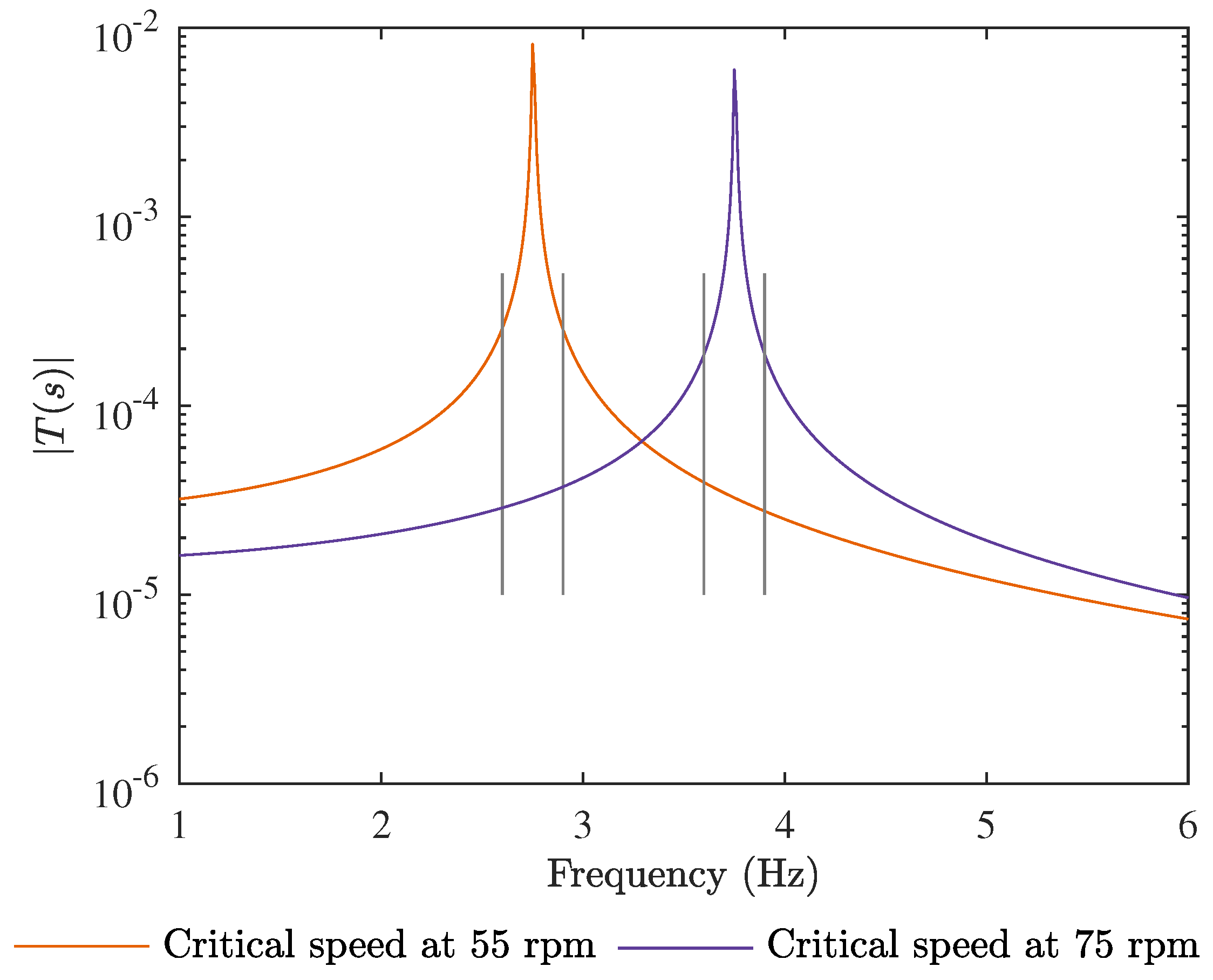
Figure 6.
Experimental results and simulation comparison for a critical speed at 55 rpm, showing the full 60-min run in (a) and a 5-min extraction in (b).
Figure 6.
Experimental results and simulation comparison for a critical speed at 55 rpm, showing the full 60-min run in (a) and a 5-min extraction in (b).
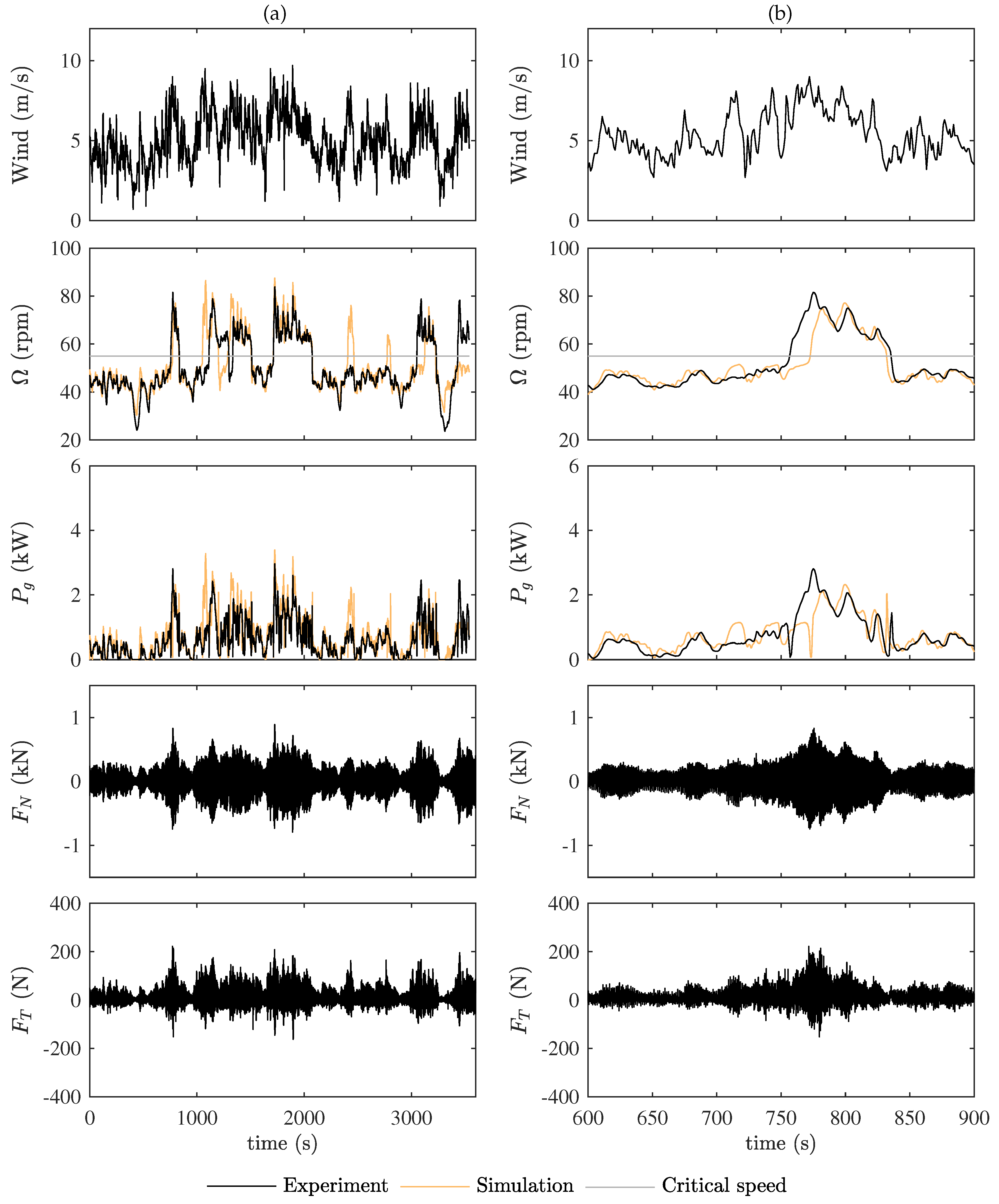
Figure 7.
Experimental results and simulation comparison for a critical speed at 75 rpm, showing the full 12-min run in (a) and a 5-min extraction in (b).
Figure 7.
Experimental results and simulation comparison for a critical speed at 75 rpm, showing the full 12-min run in (a) and a 5-min extraction in (b).
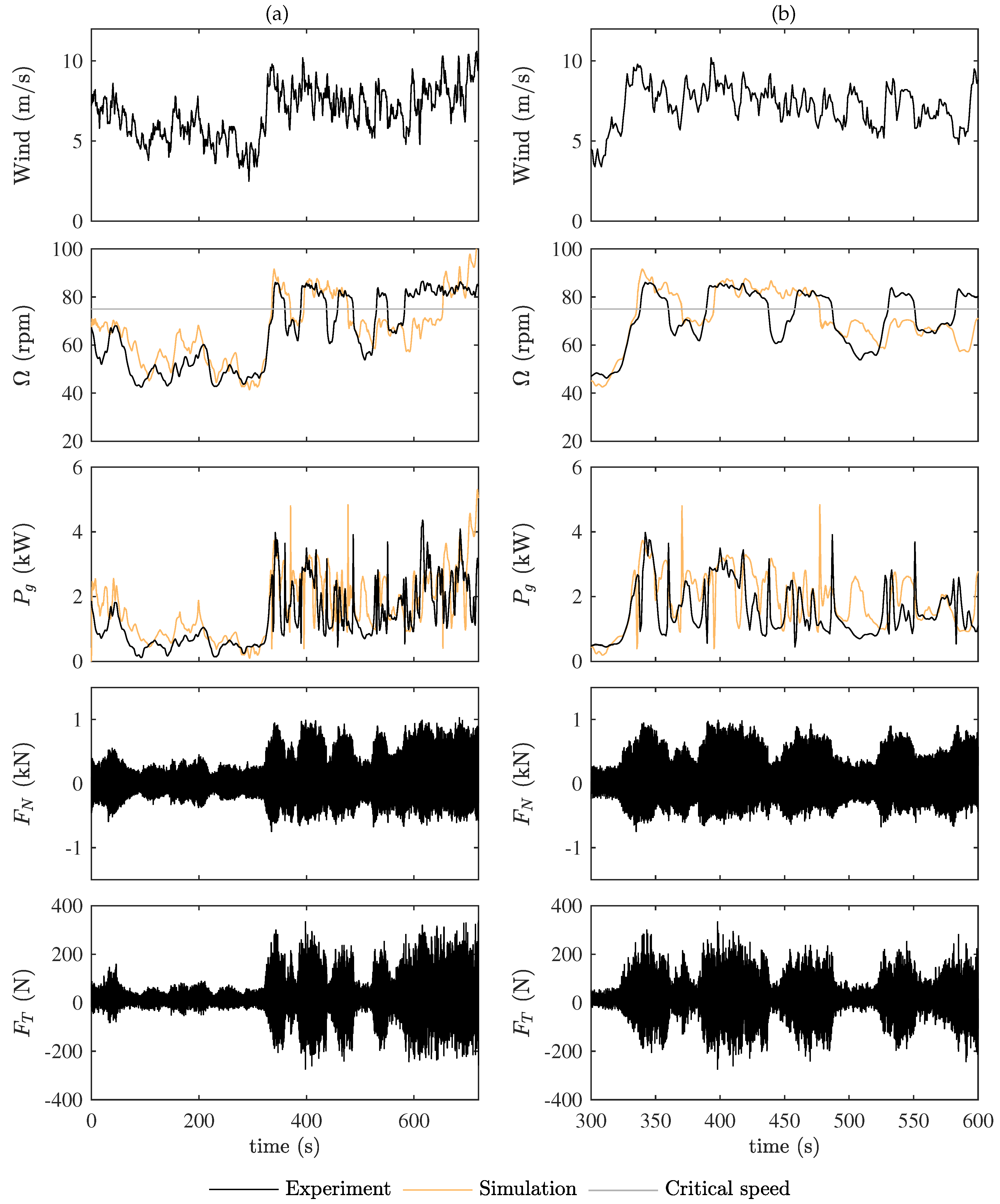
Figure 8.
Simulation with and without the critical controller activated, showing the 60-min run in (a) and a 5-min extraction in (b). The optimal rotational speed for the average of the wind speed is at 75 rpm, which is also the critical speed for exciting the tower. A total of 23 skips was performed during the 60 min, of which three skips are occurring in (b).


Table 1.
The LUT key points. The equations for hold low and hold high are derived in Appendix A.
Table 1.
The LUT key points. The equations for hold low and hold high are derived in Appendix A.
| Description | Rotational Speed, Ω | for the Low Strategy | for the High Strategy |
|---|---|---|---|
| Start * | 1 | 1 | |
| Switch-point LOW | |||
| Hold Low ** | - | ||
| Critical ** | |||
| Hold High ** | - | ||
| Switch-point HIGH | |||
| End * | 1 | 1 |
To control the spline, additional points where added: * At rad/s after the start with a value of 1.01 and at rad/s before the end with a value of 0.99. ** At rad/s with the same value as the point.
Table 2.
The design parameters for the critical speed controller.
| Parameter | Experiment | Simulation | Guide for Selection * |
|---|---|---|---|
| Hold margin, | 0.4 rad/s | Specifies the speed exclusion zone as . | |
| Switch point margin, | 0.5 rad/s | Keep close to ⇒ low risk of failed skips. | |
| Increase ⇒ smooth transaction to the hold point. | |||
| Start/end margin, | 1.0 rad/s | Low value ⇒ narrow affected range. | |
| Large value ⇒ smooth transaction to the hold point. | |||
| Critical coefficient, | 0.5 | 0.5 ** | Within 0.1–0.9. Low value ⇒ less drivetrain stress. |
| Large value ⇒ fast, ensured skips. | |||
| Hold Low coefficient, | 1.00 | 1.10 *** | Around 1. Increase ⇒ decrease skip up tendency |
| Hold High coefficient, | 1.00 | 0.85 *** | Around 1. Increase ⇒ increase skip down tendency |
* Note: . ** Additionally, a parameter sweep was simulated. *** Tuned to match the measurements.
Table 3.
System specifications.
| Rated power | 12 kW |
| Nominal rotational speed | 127 rpm |
| Nominal torque | 900 Nm |
| Number of generator pole-pairs | 16 |
| No load voltage, line to neutral | 161 V |
| DC-link capacitance | mF |
| Number of blades | 3 |
| Turbine radius, | m |
| Shaft torsion spring constant , | kNm/rad |
| Inertia of generator rotor, | kg m2 |
| Inertia of turbine, | 525 kg m2 |
| Optimal power coefficient , | 0.29 |
| Optimal tip speed ratio , | 3.4 |
| Measurement sample rate | 2 kHz |
| Rotational speed filter order | 25 |
| Rotational speed filter cutoff | p |
| Power filter order | 2 |
| Power filter cutoff | 10 Hz |
| Control loop speed | 10 Hz |
| Electric power controller loop speed | 1 kHz |
| SPWM switching frequency | kHz |
Table 4.
Simulation results of the critical speed controller based on the 60-min time series. In each case, the performance is compared to an optimal torque simulation without a critical speed.
Table 4.
Simulation results of the critical speed controller based on the 60-min time series. In each case, the performance is compared to an optimal torque simulation without a critical speed.
| Wind Optimization Method | (rpm) | No. of Skips | Critical Speed Control Compared to Optimal Power Control | ||||
|---|---|---|---|---|---|---|---|
| Energy Capture (%) | Time in Critical (%) | Power Fluctuation (%) | Tower Strength * (%) | Shaft Torque (%) | |||
| AVG | 55 | 17 | 90.8 | 8.2 | 90.6 | 70.3 | 100.0 |
| CMC | 55 | 15 | 91.9 | 7.4 | 91.8 | 75.9 | 103.1 |
| AVG | 75 | 23 | 98.2 | 7.7 | 103.7 | 76.5 | 113.9 |
| CMC | 75 | 29 | 98.3 | 8.3 | 103.4 | 75.6 | 123.4 |
* The fictive tower was designed for each case to have a natural frequency excited at .
Table 5.
Simulation results of the critical speed controller with a parameter sweep of . In each case, the performance is compared to an optimal torque simulation without a critical speed.
Table 5.
Simulation results of the critical speed controller with a parameter sweep of . In each case, the performance is compared to an optimal torque simulation without a critical speed.
| (rpm) | No. of Skips | Critical Speed Control Compared to Optimal Power Control | Max Shaft Torque (Nm) | ||||
|---|---|---|---|---|---|---|---|
| Energy Capture (%) | Time in Critical (%) | Power Fluctuation (%) | Tower Strength * (%) | ||||
| 0.2 | 55 | 17 | 90.8 | 8.8 | 90.5 | 69.3 | 456 |
| 0.3 | 55 | 17 | 90.8 | 8.6 | 90.6 | 69.8 | 456 |
| 0.4 | 55 | 17 | 90.8 | 8.4 | 90.7 | 70.3 | 456 |
| 0.5 | 55 | 17 | 90.8 | 8.2 | 90.6 | 70.3 | 456 |
| 0.6 | 55 | 17 | 90.8 | 8.1 | 91.0 | 70.1 | 456 |
| 0.7 | 55 | 17 | 90.9 | 8.0 | 91.1 | 70.1 | 470 |
| 0.8 | 55 | 17 | 90.9 | 7.9 | 91.3 | 70.1 | 519 |
| 0.2 | 75 | 23 | 98.2 | 8.7 | 103.0 | 77.2 | 679 |
| 0.3 | 75 | 23 | 98.2 | 8.3 | 103.2 | 77.3 | 679 |
| 0.4 | 75 | 23 | 98.2 | 8.0 | 103.6 | 77.2 | 724 |
| 0.5 | 75 | 23 | 98.2 | 7.7 | 103.7 | 76.5 | 774 |
| 0.6 | 75 | 23 | 98.2 | 7.4 | 104.1 | 75.8 | 821 |
| 0.7 | 75 | 23 | 98.3 | 7.2 | 104.1 | 75.2 | 903 |
| 0.8 | 75 | 23 | 98.3 | 7.1 | 104.4 | 75.0 | 980 |
* The fictive tower was designed for each case to have a natural frequency excited at .
© 2017 by the authors. Licensee MDPI, Basel, Switzerland. This article is an open access article distributed under the terms and conditions of the Creative Commons Attribution (CC BY) license (http://creativecommons.org/licenses/by/4.0/).
Share and Cite
MDPI and ACS Style
Rossander, M.; Goude, A.; Eriksson, S. Critical Speed Control for a Fixed Blade Variable Speed Wind Turbine. Energies 2017, 10, 1699. https://doi.org/10.3390/en10111699
AMA Style
Rossander M, Goude A, Eriksson S. Critical Speed Control for a Fixed Blade Variable Speed Wind Turbine. Energies. 2017; 10(11):1699. https://doi.org/10.3390/en10111699
Chicago/Turabian StyleRossander, Morgan, Anders Goude, and Sandra Eriksson. 2017. "Critical Speed Control for a Fixed Blade Variable Speed Wind Turbine" Energies 10, no. 11: 1699. https://doi.org/10.3390/en10111699
Note that from the first issue of 2016, this journal uses article numbers instead of page numbers. See further details here.