
Grid-Connected Control Strategy of Five-level Inverter Based on Passive E-L Model


College of Automation Engineering, Shanghai University of Electric Power, Shanghai 200090, China
*
Author to whom correspondence should be addressed.
Energies 2017, 10(10), 1657; https://doi.org/10.3390/en10101657
Submission received: 20 September 2017
/
Revised: 16 October 2017
/
Accepted: 18 October 2017
/
Published: 19 October 2017
(This article belongs to the Special Issue Emerging Power Electronics Technologies for Power Systems and Machine Drives)
Abstract
:At present, the research on five-level inverters mainly involves the modulation algorithm and topology, and few articles study the five-level inverter from the control strategy. In this paper, the nonlinear passivity-based control (PBC) method is proposed for single-phase uninterruptible power supply inverters. The proposed PBC method is based on an energy shaping and damping injection idea, which is performed to regulate the energy flow of an inverter to a desired level and to assure global asymptotic stability, respectively. Furthermore, this paper presents a control algorithm based on the theory of passivity that gives an inverter in a photovoltaic system additional functions: power factor correction, harmonic currents compensation, and the ability to stabilize the system under varying injection damping. Finally, the effectiveness of the PBC method in terms of both stability and harmonic distortion is verified by the simulation and experiments under resistive and inductive loads.
1. Introduction
Recently, an effort to extend the scope of the applications of multilevel inverters to clean energy harnessing from photovoltaic arrays and fuel cells has also been pursued, wherein their superior harmonic performance and ability to support independent maximum power point tracking are advantages noted for these lower voltage implementations [1,2,3,4]. For high-voltage energy conversion, multilevel inverters are viewed as the preferred topological solutions compared to the traditional two-level inverter bridge because of their many associated advantages, including reduced semiconductor voltage stress, improved harmonic performance, and reduced electromangnetic interference [5,6]. The conventional multilevel converters are mainly divided into three types: neutral-point-clamped (NPC) inverter, flying capacitor (FC) inverter, and cascaded H-bridge (CHB) inverter. Many papers focus on the NPC inverter, which has found widespread use in active filters, renewable energy conversion systems, and traction motor applications [7,8,9,10,11,12,13,14,15].
In the literature, numerous modulation techniques have been proposed to obtain the inverter output voltage nearing a perfect sinusoidal waveform. Several modulation techniques have been proposed for reducing harmonics and minimizing switching losses for NPC inverters. The modulation methods for NPC inverters can be classified according to switching frequencies: (a) Space Vector Modulation (SVM); (b) Phase Shifted PWM; and (c) Level Shifted PWM. Among these, SVM helps in the good utilization of DC link voltage and lower current ripples. However, with a higher number of voltage levels, the complexity of choosing a switching state increases as the redundancy of the switching state increases. A level shifted modulation scheme consists of triangular carriers which are vertically shifted. The total harmonic distortion (THD) of phase-shifted modulation is much higher than that of the level shifted technique. Therefore, level shifted modulation is considered in this paper [16,17,18,19].
With the advance of classical control theory and modern control theory, Proportional Intergral (PI) control, Proportional Resonant (PR) control and sliding mode control are applied to the control of the inverter. To some extent, these methods can solve some problems. However, as the complexity and coupling of the system increase, these methods have been unable to meet the demand [20,21,22]. The authors of [23] proposed a deadbeat control strategy. Although the method provides a very fast dynamic response, it is not robust to the parameter variations, which may adversely affect the performance. In the literature [24], adaptive controls are applicable to the control of the inverter. This method has important advantages such as eliminating the sensitive error, ensuring that the transfer function of the controller is not changed, and improving the control performance of the system. However, the predicted value of the grid-impedance is difficult to ascertain. The authors of [25] proposed a sliding mode control strategy. The control algorithm can improve the robustness of the system and hold a superior practical value. However, variable switching frequency, steady-state error in the output voltage, and chattering are the main drawbacks of this method. Furthermore, the constant sliding gain results in a static sliding line, which leads to insufficient dynamic responses during load transients.
The aforementioned control methods offer various advantages and disadvantages related to dynamic response, robustness aginst parameter variations, steady-state error, and stability. The common disadvantage is that they do not take into consideration the energy dissipation properties of the inverter, which are inherently imposed by its physical structure. In order to implement the nonlinear control of power electronic devices, passivity-based control (PBC) theory has been applied to the control of the inverter and has achieved a good control effect [26,27]. In the literature [28], it is noted that PBC strategy can improve the dynamic and static characteristics of the system, which also has strong robustness to parameter changes. In the literature [29], the passivity-based control has better robustness and dynamics compared with traditional PI control. In the literature [30], PBC strategy has a fast dynamic response compared with the droop control, which can improve the stability of the system. The literature [31] proposes that passivity-based control (PBC) can simplify the control algorithm, which has a high anti-perturbation reaction to the parameter change in contrast with the traditional vector control.
At present, the research on the five-level inverter mainly involves the modulation algorithm and topology, and few articles study it with the control strategy. In this paper, passivity-based control is introduced to the system of the five-level inverter for the first time. Firstly, the mathematical model of the five-level inverter is deduced by the topological structure and the switching function. Then, the function expression of the passive E-L model can be derived by selecting the appropriate energy function and the damping injection, which combines with the Sinusoidal Pulse Width Modulation (SPWM) algorithm to drive the switch of the inverter. Finally, PBC strategy was compared with the traditional PI control through simulation software, and the results have been analyzed. Meanwhile, the validity of the control strategy based on passive Euler (E-L) model is also verified by the prototype experiment.
2. Topology and Mathematical Mode
2.1. Topology
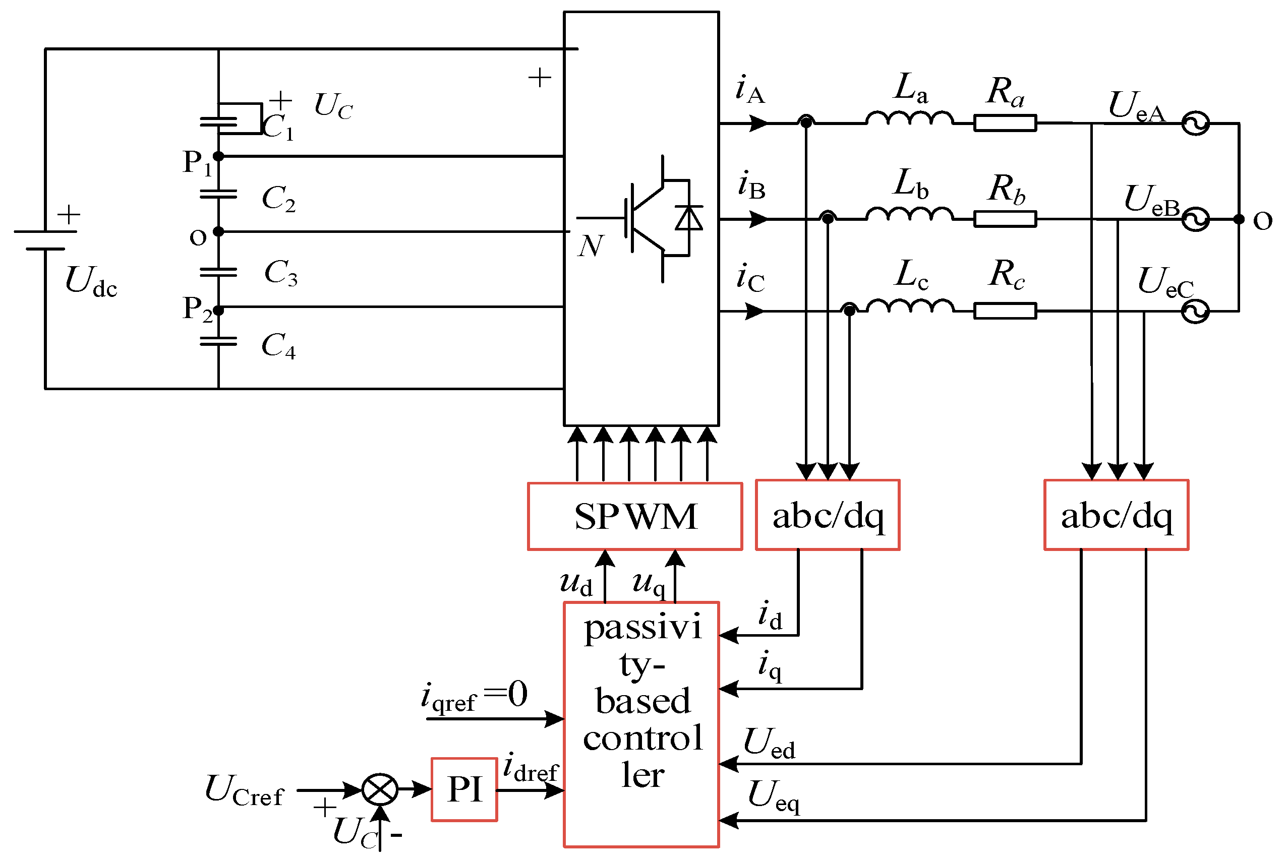
Figure 1 showed the grid-connected system of the single-stage, three-phase, diode-clamped, five-level inverter. The equivalent resistances of the system are Ra, Rb, and Rc, and the equivalent inductors are La, Lb, and Lc. Further, Ra = Rb = Rc = R, and La = Lb = Lc = Lf. C1 = C2 = C3 = C4 = C is the polar film capacitor between the DC stack buses. The voltage of the DC side is Udc. Idc denotes the current from the DC-link to the inverter. TA1–TA8, TB1–TB8, and TC1–TC8 are the eight switches on the arms of phases A, B, and C respectively. VA1–VA6, VB1–VB6, and VC1–VC6 are the six clamp diodes on the arms of phases A, B, and C respectively. SA, SB, and SC are the switch signals of each arm on the phases A, B, and C respectively. Among them, the switch signals of the arm on phase A are SA1, SA2, SA3, SA4, SA5, SA6, SA7, and SA8. Likewise, the switch signals of phase B and phase C can be obtained. UeA, UeB, and UeC denote the grid side AC voltages.
2.2. Working Principle
The five-level inverter has a variety of working methods according to the switch sequence. Taking phase A as an example to explain its working principle:
- (1)
- TA1, TA2, TA3, and TA4 shut down at the same time; TA5, TA6, TA7, and TA8 switch on at the same time; and then the output phase voltage of the inverter is +Udc/2 and SA = +2.
- (2)
- TA2, TA3, TA4, and TA5 shut down at the same time; TA1, TA6, TA7, and TA8 switch on at the same time; and then the output phase voltage of the inverter is +Udc/4 and SA = +1.
- (3)
- TA3, TA4, TA5, and TA6 shut down at the same time, and TA1, TA2, TA7, and TA8 switch on at the same time. O point and N point have the same potential at the same moment, so the output phase voltage of the inverter is 0. Meanwhile, SA = 0.
- (4)
- TA4, TA5, TA6, and TA7 shutdown at the same time; TA1, TA2, TA3, and TA8 switch on at the same time; and the output phase voltage of the inverter is −Udc/4 and SA = −1.
- (5)
- TA5, TA6, TA7, and TA8 shut down at the same time; TA1, TA2, TA3, and TA4 switch on at the same time; and the output phase voltage of the inverter is −Udc/2 and SA = −2.
2.3. Mathematical Model
Assuming that the opening state of the switch is 0 and the closing state is 1, the penta-state switching function Sk can be decomposed into eight two-state switching functions, as in Equation (1).
where the subscript k = A, B, C.
The mathematical model of the five-level inverter in the static a-b-c frame can be derived as:
Among them,
where UC1 and UC4 are the voltages of the capacitors C1 and C4 in the DC side, respectively, and iA, iB, and iC are the three-phase current of the inverter.
After the coordinate transformation, the mathematical model of the five-level inverter in the dq rotation coordinate is [32,33,34]:
where id and iq are the three-phase current in the rotation d-q frame; Ued and Ueq are the grid-connected voltage in the rotation d-q frame; Sd1, Sq1 and Sd2, Sq2 are the coordinate components of SA1 and SA2 in the rotation d-q frame; Sd7, Sq7 and Sd8, Sq8 are the coordinate components of SA7 and SA8 in the rotation d-q frame; and ω is the angular speed of rotation.
3. SPWM Modulation Strategy
Sinusoidal pulse width modulation (SPWM) strategies have been used widely for the switching of multilevel inverters due to their simplicity, flexibility, and reduced computational requirements compared to space vector modulation (SVM). Multilevel voltage source inverter systems offer the advantages of realizing higher voltages using smaller rating switching devices; they also achieve better quality output voltage waveforms compared to the use of two-level inversion systems. There are different modulation techniques based on the SPWM scheme; the carrier-based modulation schemes for multilevel inverters require carrier signals. They can be generally classified into two categories: phase-shifted and level-shifted modulations. In phase-shifted modulation, all the triangular carriers have the same frequency and the same amplitude, but there is a phase shift anger between any two adjacent carrier waves.
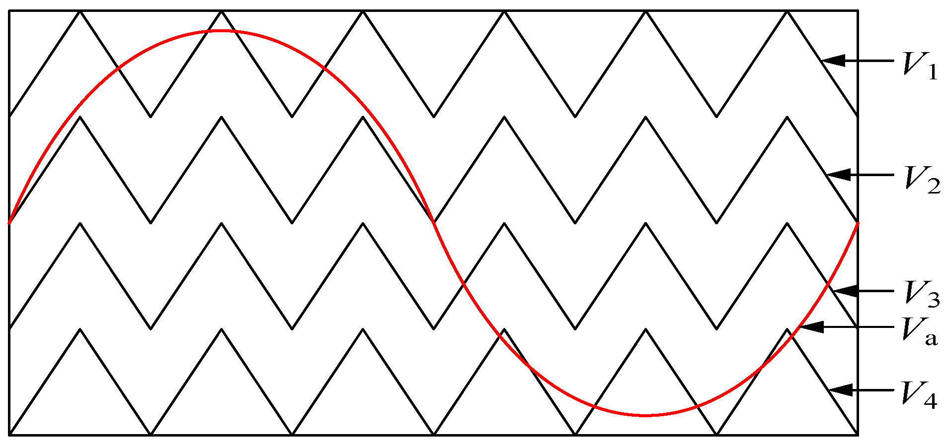
There are basically three types of schemes for the level-shifted modulation, which are as follows: In-phase disposition (IPD), Alternative phase opposite disposition (APOD), and Phase opposite disposition (POD). In the In-phase disposition (IPD) modulation, see Figure 2, each phase uses a sinusoidal modulation wave to compare a plurality of triangular carrier waves in a multilevel inverter. When the amplitude of the sine wave is greater than the amplitude of the carrier wave, the switch is closed. On the contrary, when the amplitude of the sine wave is lower than the amplitude of the carrier wave, the switch is opened.
In Figure 2, Va is the amplitude of the sinusoidal modulation wave, and V1 to V4 are the amplitudes of the same phase triangular wave. Among them, V1 controls TA1 and TA5, V2 controls TA2 and TA6, V3 controls TA3 and TA7, and V4 controls TA4 and TA8. When the amplitude of the sine wave Va is greater than the amplitude of the triangular carrier wave V1 to V4, the switching of each phase is shut down. On the contrary, when Va is smaller than V1 to V4, the switching is switched on.
4. Design of Passive Controller
4.1. Passive E-L Model of the Five-Level Inverter
Selecting the system’s state variables:
Defining the energy storage function of the system:
Equation (4) is written in the form of the E-L equation under passivity-based controls (see Figure 1) [35,36].
Among them,
where x is the state variable, u is the control variable that reflects the exchange between the system and the external energy, M is a positive diagonal matrix consisting of energy storage elements, J is the anti-symmetric matrix that reflects the internal interconnection structure of the system, J is equal to −JT, and R is the symmetric matrix that reflects the dissipation characteristics of the system.
4.2. Design of Passive E-L Model Controller
For an m input and m output system:
where x, u, and y are the state variables, input variables, and output variables of the system, respectively; the spaces are x ∈ Rn, u ∈ Rm, and y ∈ Rm, respectively; and f is the local Lipschitz about (x, u).
If there is a semi-definite and continuously differentiable storage function H(x) and a positive definite function Q(x) for t > 0, the dissipation inequality is satisfied:
or
The system is strictly passive if the input u, the output y and the energy supply rate uTy are established.
For the inverter system represented by Equation (4), we can set to its storage function as . Then it can be deduced:
Assuming that y = x, Q(x) = xTRx, it can be concluded that the system satisfies the strict passive inequality.
If xe = x − x*, it can be deduced from Equation (7):
where x* is the desired equilibrium point in the system. It can be expressed as:
where idref and iqref are the expected components in the d and q axis of the three-phase current iA, iB, and iC. UC1ref and UC4ref are the expected voltages of the capacitors C1 and C4 in the DC side, respectively.
Generally, the method of injected damping can be used to control xe quickly becoming zero. The injected damping dissipation term is:
where Ra is a semi-definite diagonal matrix that is similar to the form of matrix R and Ra = [Ra1 Ra2 Ra3 Ra4]. Equation (12) can be rewritten as:
Rd xe = (R + Ra)xe
In order to ensure the strict passivity of the system, we can select the control law:
When , the error energy function is:
Combining Equation (4) with Equation (7) to solve Equation (16), it can be deduced:
With ud and uq, the input signal from the SPWM algorithm can be obtained from Equation (4):
Combined with the Equations (18) and (19), it can be deduced:
In summary, the block diagram of the system under passivity-based control can be established. In Figure 3, the q-axis desired current iqref is equal to 0 in order to ensure that the unit power factor is connected to the grid. The d-axis desired current idref is obtained by the difference between the actual capacitor voltage and the expected capacitor voltage through PI control.
5. Software Simulation
5.1. Simulation of Passivity Control Mentioned in This Paper
According to the above analysis, a simulation model of passivity-based control based on the E-L model is built in Matlab/Simulink simulation software. The simulation parameter specifications are given in Table 1.
The output phase voltage and line voltage waveform of the inverter are presented in Figure 4a,b, respectively. It can be seen from Figure 4a that the phase voltage, which consists of +300 V, +150 V, 0 V, −150 V, and −300 V, is respectively close to the five levels of the inverter output in theory, which are +Udc/2, +Udc/4, 0, −Udc/4, and −Udc/2. Similarly, Figure 4b shows that the line voltage consists of +600 V, +450 V, +300 V, +150 V, 0 V, −150 V, −300 V, −450 V, and −600 V, which is respectively close to the nine levels of the inverter output in theory, which are +Udc, +Udc3/4, +Udc/2, +Udc/4, 0, −Udc/4, −Udc/2, −Udc3/4, and −Udc.
The outputs functions ud and uq from the passive controller, when the injection damping Ra1 = Ra2 = Ra = 5 Ω, 15 Ω, 25 Ω, 50 Ω, and 100 Ω, are shown in Figure 4c,d, respectively. In Figure 4c, when Ra ≤ 25 Ω, ud tends to be stable at about 0.005 s, and, when Ra > 25 Ω, the stability time of ud is significantly greater than 0.01 s. Among them, when Ra = 50 Ω, ud tends to be stable at about 0.02 s, and, when Ra = 100 Ω, the stability time is about 0.04 s.
In Figure 4d, when Ra ≤ 25 Ω, uq tends to be stable about 0.01 s, and the stability time of the output function uq is longer than 0.01 s, when Ra > 25 Ω. Especially, when Ra = 50 Ω, uq tends to be stable at about 0.02 s, and, when Ra = 100 Ω, uq does not reach stability at 0.04 s.
Considering the steady-state response speed of the system, it is reasonable to select Ra1 = Ra2 = Ra = 25 Ω.
5.2. The Passivity-Based Control of This Paper Is Compared with the Traditional PI Control
In order to demonstrate the advantages of the passivity-based control proposed in this paper, this paper compares it with traditional PI control. Among these, the input of the PI controller of the voltage loop is the difference between the actual capacitor voltage and the reference capacitor voltage, and the main purpose is to track the capacitor voltage and inhabit the capacitor voltage offset. Meanwhile, the value of Kp is relatively small and the value of Ki is relatively large, which ensures the accuracy of voltage tracking. The function of the PI controller of the current loop is to track the three-phase grid current and voltage. If Kp is too large, the stability of the system is poor. In summary, we select Kp = 0.8 and Ki = 5.
The active power P from the inverter is shown in Figure 5a,b under two strategies. As can be seen from the figure, P tends to be stable at about 0.01 s, and the stability value is close to 8000 W under the two control strategies. However, the amplitude fluctuations of the active power in Figure 5b are obviously larger than those in Figure 5a. It can be concluded that the static stability of the passivity-based control strategy is good.
The currents in the d-axis direction inside the passive controller under different injection dampings that are shown in Figure 5c are obtained by the three-phase current of the inverter through the abc-dq coordinate transformation. It can be observed in Figure 5c, with the increase of the injection damping, that the stability time of the current id is getting smaller and smaller. Especially, when Ra ≥ 25 Ω, the stability time is close to 0.003 s. Meanwhile, the fluctuation range of id is getting smaller, and the dynamic stability is getting higher.
The resistances in the traditional PI control system are set to 5 Ω, 15 Ω, 25 Ω, 50 Ω, and 100 Ω, which is contrast with the dynamic simulation of different injection dampings under the passivity-based control strategy. Figure 5d shows that the current id is under different resistances in the traditional PI control system. It can be seen from Figure 5d that, when Ra ≤ 25 Ω, id tends to be stable at 0.01 s. When Ra = 50 Ω, id tends to be stable at about 0.02 s, and, when Ra = 100 Ω, id does not reach stability at 0.04 s.
Compared with Figure 5c, the stability time of the current id is significantly longer in Figure 5d. Meanwhile, the magnitude of the current amplitude fluctuates considerably in Figure 5c. In summary, the dynamic stability of passivity-based control is better than that of traditional PI control.
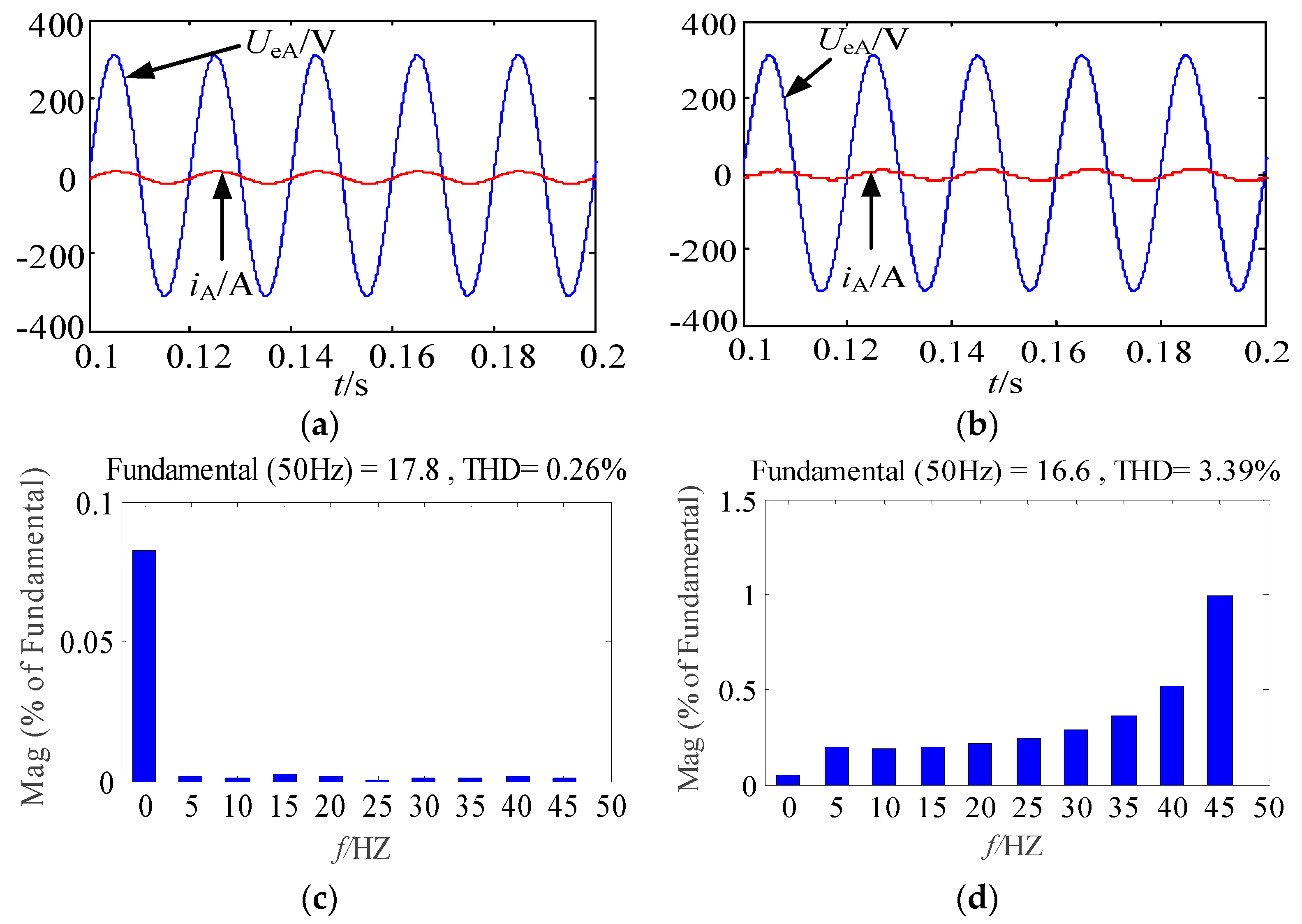
A-phase grid voltage and current are shown in Figure 6a,b under two kinds of strategies. In Figure 6b, the current tends to be stable at about 0.1 s, and there is a certain phase difference between the grid voltage and current after stabilization. At this point, the system’s power factor is very low. However, the grid current achieves stability in a very short period of time in Figure 6a. Meanwhile, there is a smaller phase difference between the grid voltage and current; thus the system’s power factor is higher.
Figure 6c,d compares the harmonics of the grid currents controlled by the PBC strategy and the traditional PI control methods. It can be seen from the two figures that the harmonics of the A-phase current are 0.26% and 3.39% under two strategies, respectively. The results show that the typical harmonic in the grid current by the PBC method is smaller than that by the traditional PI control method due to the superior stability performance.
Table 3 shows the stability and harmonic results of the two control strategies.
6. Prototype Experiment
In order to further illustrate the advantages of this method, this paper also builds the hardware experiment platform of the inverter. Meanwhile, an experimental analysis based on passivity-based control is also carried out on this platform. In the experiment, the micro-power supply is replaced by the DC power supply. The control signal is generated by the Digital Signal Processingn (DSP) controller of the TMS320F28335 (Texas Instruments, Dallas, TX, USA) type, and the switching device is the Infineon IKW40N120H3 (TrenchStop, Infineon, Germany). Meanwhile, the hard experiments using the same simulation specifications are given Table 1. The hardware experiment is shown in Figure 7.
The A-phase grid voltage and current are shown in Figure 8a,b under two kinds of strategies. In Figure 8a, the A-phase grid voltage is substantially in the same phase with the current of the inverter. At this point, the system has a better grid power factor. However, there is a certain phase difference between grid voltage and the current in Figure 8b. Therefore, the system’s power factor is higher under the passivity-based control strategy. Meanwhile, compared with the software simulation, the voltage and current in Figure 8a are approximately consistent with the waveform in Figure 6a, which proves that the passive control strategy has a higher power factor. The waveform of voltage and current is affected proportional to the parameters and integral parameters in the PI controller, and it is difficult to find the most accurate PI parameters that meet the control requirements. Therefore, there is a phase difference between the voltage and the current of Figure 6b and Figure 8b.
Figure 8c shows the d-axis current in the two kinds of strategies under different injection damping, which is obtained by the three-phase current of the inverter through the abc-dq coordinates transformation. In the Figure 8c, there is a certain fluctuation after the current reaches the stability under the two strategies. Especially, when Ra ≤ 25 Ω, the magnitude of the current amplitude fluctuates considerably. However, the ring of the fluctuation is significantly smaller under the PBC strategy, which proves that a passivity-based control strategy has good dynamic stability.
Figure 8d shows the polar film capacitor voltage under the PBC strategy. Here, UC1, UC2, UC3, and UC4 are the voltages of the capacitors C1, C2, C3, and C4 in the DC side, respectively. The capacitor voltage in the figure is close to 150 V, which proves that the problem of the balance of the neutral point is relatively small.
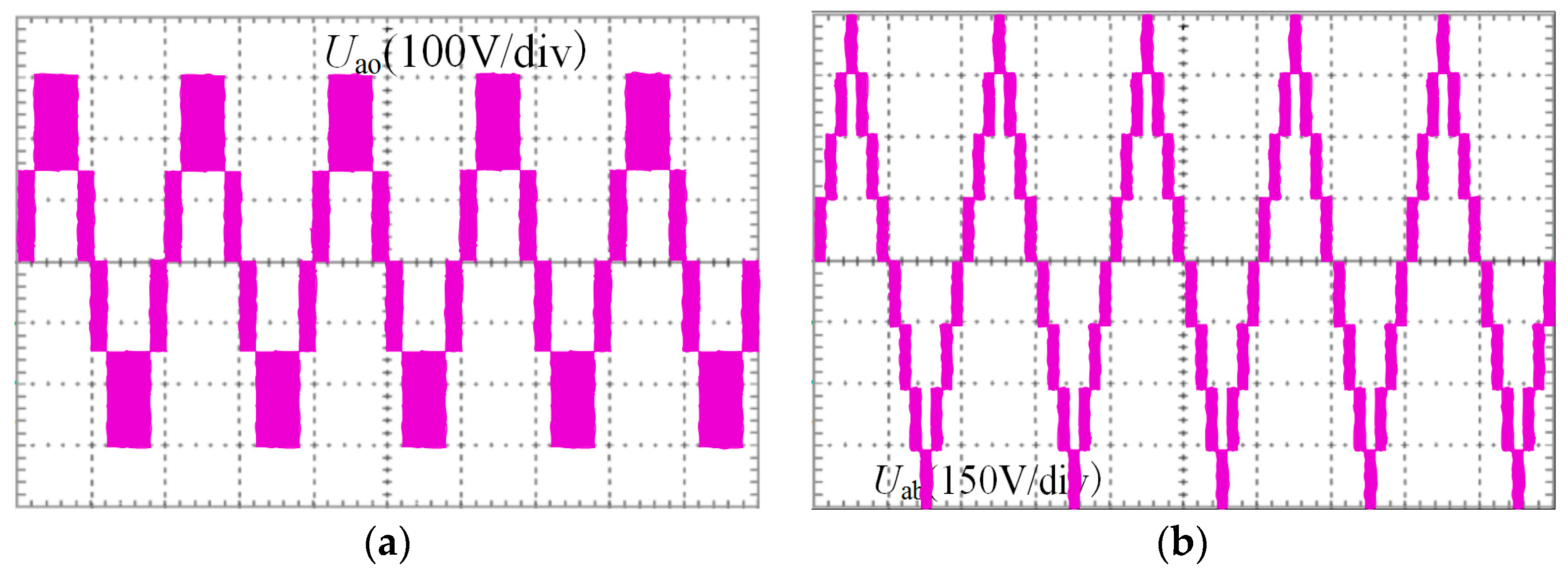
The output phase voltage and the line voltage waveform of the inverter are presented in Figure 9a,b, respectively. It can be seen from Figure 9a that the output phase voltage consisted of +300 V, +150 V, 0 V, −150 V, and −300 V and is close to the five levels of the inverter output in theory, which are +Udc/2, +Udc/4, 0, −Udc/4, and −Udc/2. Similarly, Figure 9b shows that the output line voltage consists of +600 V, +450 V, +300 V, +150 V, 0 V, −150 V, −300 V, −450 V, and −600 V. Meanwhile, the experimental results are approximately consistent with the results obtained in the software simulation.
7. Conclusions
This paper is related to a grid-connected control strategy of the five-level inverter based on a passive E-L model. Firstly, the mathematical model of the five-level inverter is deduced through the topological structure and the switching function. Then, the passive control law can be derived by selecting the appropriate energy function and the injection damping, which combines with the SPWM algorithm to drive the switch. Finally, the software simulation and hardware experiments draw the following conclusions:
- (1)
- The optimum stability of the system can be achieved by selecting the appropriate energy function and injection damping.
- (2)
- Compared with the traditional PI control method, the passivity-based control strategy has better static and dynamic stability and makes the system achieve a higher power factor.
- (3)
- In terms of economy, the harmonic loss very small under passivity-based control.
Acknowledgments
This work was supported by the National Natural Science Foundation of China (61573239), The Key Science and Technology Plan of Shanghai Science and Technology Commission (14110500700), and the Natural Science Foundation of Shanghai (15ZR1418600).
Author Contributions
The paper was a collaborative effort between the authors. The authors contributed collectively to the theoretical analysis, modeling, simulation, and manuscript preparation.
Conflicts of Interest
The authors declare no conflicts of interest.
References
- Mokhtar, A.; Ahmed, E.M.; Masahito, S. Thermal Stresses Relief Carrier-Based PWM Strategy for Single-Phase Multilevel Inverters. IEEE Trans. Power Electron. 2017, 32, 9376–9388. [Google Scholar]
- Wang, H.; Liu, Y.; Sen, P.C. A neutral point clamped multilevel topology flow graph and space NPC multilevel topology. In Proceedings of the 2015 IEEE Energy Conversion Congress and Exposition (ECCE), Montreal, QC, Canada, 20–24 September 2015; pp. 3615–3621. [Google Scholar]
- Ahmed, M.; Zainal, S.; Amjad, A.M. Harmonics elimination PWM based direct control for 23-level multilevel distribution STATCOM using differential evolution algorithm. Electr. Power Syst. Res. 2017, 152, 48–60. [Google Scholar]
- Georgios, K.; Josep, P.; Daniel, P. A Hybrid Modular Multilevel Converter with Partial Embedded Energy Storage. Energies 2016, 9, 12. [Google Scholar]
- Lee, K.S.; Oh, G.; Chu, D.; Pak, S.W.; Kim, E.K. High power conversion efficiency of intermediate band photovoltaic solar cell based on Cr-doped ZnTe. Sol. Energy Mater. Sol. Cells 2017, 170, 27–32. [Google Scholar] [CrossRef]
- Genevieve, S.; Julian, C. Subsidies for residential solar photovoltaic energy systems in Western Australia: Distributional, procedural and outcome justice. Renew. Sustain. Energy Rev. 2016, 65, 262–273. [Google Scholar]
- Gupta, K.K.; Ranjan, A.; Bhatnagar, P.; Sahu, L.; Jain, S. Multilevel inverter topologies with reduced device count: A review. IEEE Trans. Power Electron. 2016, 31, 135–151. [Google Scholar] [CrossRef]
- Hu, C.; Yu, X.; Holmes, D.G.; Shen, W.; Wang, Q.; Luo, F.; Liu, N. An Improved Virtual Space Vector Modulation Scheme for Three-Level Active Neutral-Point-Clamped Inverter. IEEE Trans. Power Electron. 2017, 32, 7419–7434. [Google Scholar] [CrossRef]
- Xia, C.; Zhang, G.; Yan, Y.; Gu, X.; Shi, T.; He, X. Discontinuous Space Vector PWM Strategy of Neutral-Point-Clamped Three-Level Inverters for Output Current Ripple Reduction. IEEE Trans. Power Electron. 2017, 32, 5109–5121. [Google Scholar] [CrossRef]
- Song, K.; Georgios, K.; Li, J.; Wu, M.; Vassilios, G.A. High performance control strategy for single-phase three-level neutral-point-clamped traction four-quadrant converters. IET Power Electron. 2017, 10, 884–893. [Google Scholar]
- Lei, Y.; Barth, C.; Qin, S.; Liu, W.-C.; Moon, I.; Stillwell, A.; Chou, D.; Foulkes, T.; Ye, Z.; Liao, Z.; et al. A 2-kW Single-Phase Seven-Level Flying Capacitor Multilevel Inverter with an Active Energy Buffer. IEEE Trans. Power Electron. 2017, 32, 8570–8581. [Google Scholar] [CrossRef]
- Dekka, A.; Wu, B.; Zargari, N.R. Start-Up Operation of a Modular Multilevel Converter with Flying Capacitor Submodules. IEEE Trans. Power Electron. 2017, 32, 5873–5877. [Google Scholar] [CrossRef]
- Liangzong, H.; Chen, C. A Flying-Capacitor-Clamped Five-Level Inverter Based on Bridge Modular Switched-Capacitor Topology. IEEE Trans. Ind. Electron. 2016, 63, 7814–7822. [Google Scholar]
- Youngjong, K.; Markus, A.; Giampaolo, B. Power Routing for Cascaded H-Bridge Converters. IEEE Trans. Power Electron. 2017, 32, 9435–9446. [Google Scholar]
- Saeed, O.; Reza, Z.M.; Masih, K. Improvement of Post-Fault Performance of a Cascaded H-bridge Multilevel Inverter. IEEE Trans. Ind. Electron. 2017, 64, 2779–2788. [Google Scholar]
- Sheng, X.; Zhendong, J. A Study of the SPWM High-Frequency Harmonic Circulating Currents in Modular Inverters. J. Power Electron. 2016, 16, 2119–2128. [Google Scholar]
- Liu, Z.; Zheng, Z.; Sudhoff, S.D.; Gu, C.; Li, Y. Reduction of Common-Mode Voltage in Multiphase Two-Level Inverters Using SPWM with Phase-Shifted Carriers. IEEE Trans. Power Electron. 2015, 31, 6631–6645. [Google Scholar] [CrossRef]
- Jacob, L.; Behrooz, M. An Adaptive SPWM Technique for Cascaded Multilevel Converters with Time-Variant DC Sources. IEEE Trans. Ind. Appl. 2016, 52, 4146–4155. [Google Scholar]
- Dong, X.; Yu, X.; Yuan, Z.; Xia, Y.; Li, Y. An Improved SPWM Strategy to Reduce Switching in Cascaded Multilevel Inverters. J. Power Electron. 2016, 16, 490–497. [Google Scholar] [CrossRef]
- Niu, L.; Xu, D.; Yang, M.; Gui, X.; Liu, Z. On-line inertia identification algorithm for pi parameters optimization in speed loop. IEEE Trans. Power Electron. 2015, 30, 849–859. [Google Scholar] [CrossRef]
- Li, B.; Zhang, M.; Huang, L.; Hang, L.; Tolbert, L.M. A robust multi-resonant PR regulator for three-phase grid-connected VSI using direct pole placement design strategy. In Proceedings of the IEEE Applied Power Electronics Conference and Exposition (APEC), Long Beach, CA, USA, 17–21 March 2013; pp. 960–966. [Google Scholar]
- Zhang, X.; Sun, L.; Zhao, K.; Sun, L. Nonlinear speed control for PMSM system using sliding-mode control and disturbance compensation techniques. IEEE Trans. Power Electron. 2013, 28, 1358–1365. [Google Scholar] [CrossRef]
- Pichan, M.; Rastegar, H.; Monfared, M. Deadbeat control of the stand-alone four-leg inverter considering the effect of the neutral line inductor. IEEE Trans. Ind. Electron. 2017, 64, 2592–2601. [Google Scholar] [CrossRef]
- Mahmood, H.; Michaelson, D.; Jiang, J. Accurate reactive power sharing in an islanded microgrid using adaptive virtual impedances. IEEE Trans. Power Electron. 2015, 30, 1605–1617. [Google Scholar] [CrossRef]
- Abrishamifar, A.; Ahmad, A.A.; Mohamadian, M. Fixed switching frequency sliding mode control for single-phase unipolar inverters. IEEE Trans. Power Electron. 2012, 27, 2507–2514. [Google Scholar] [CrossRef]
- Harnefors, L.; Wang, X.; Yepes, A.G.; Blaabjerg, F. Passivity-based stability assessment of grid-connected VSCs—An overview. IEEE J. Emerg. Sel. Top. Power Electron. 2016, 4, 116–125. [Google Scholar] [CrossRef]
- Harnefors, L.; Yepes, A.G.; Vidal, A.; Doval-Gandoy, J. Passivity-based controller design of grid-connected VSCs for prevention of electrical resonance instability. IEEE Trans. Ind. Electron. 2015, 62, 702–710. [Google Scholar] [CrossRef]
- Santos, G.V.; Cupertino, A.F.; Mendes, V.F.; Seleme, S.I. Interconnection and damping assignment passivity-based control of a PMSG based wind turbine for maximum power tracking. In Proceedings of the 2015 IEEE 24th International Symposium on Industrial Electronics (ISIE), Rio de Janeiro, Brazil, 3–5 June 2015; pp. 306–311. [Google Scholar]
- Hou, R.S.; Hui, H.; Nguyen, T.T. Robustness improvement of superconducting magnetic energy storage system in microgrids using an energy shaping passivity-based control strategy. Energies 2017, 10, 5. [Google Scholar] [CrossRef]
- Liu, X.B.; Li, C.B.; Sun, K. Voltage support for industrial distribution network by using positive/negative sequence passivity-based control. In Proceedings of the 2016 IEEE 8th International Power Electronics and Motion Control Conference (IPEMC-ECCE Asia), Hefei, China, 22–26 June 2016; pp. 674–679. [Google Scholar]
- Ramrez-Leyva, F.H.; Peralta-Sanchez, E.; Vasquez-Sanjuan, J.J.; Trujillo-Romero, F. Passivity–Based Speed Control for Permanent Magnet Motors. Procedia Technol. 2013, 7, 215–222. [Google Scholar] [CrossRef]
- Baile, Z.; Jiuhe, W.; Fengjiao, Z. The PCHD model and control of TNPC PV grid-connected inverter. Proc. CSEE 2014, 34, 204–210. [Google Scholar]
- Zhang, Z.; Liu, X.; Wang, C.; Kang, L.; Liu, H. A Passivity-based Power Control for a Three-Phase Three-level NPC Rectifier. In Proceedings of the International Conference on Electrical Machines and Systems (ICEMS), Pattaya, Thailand, 25–28 October 2015; pp. 383–386. [Google Scholar]
- Cao, Y.J.; Xu, Y.; Li, Y.; Yu, J.Q. A Lyapunov Stability Theory-Based Control Strategy for Three-Level Shunt Active Power Filter. Energies 2017, 10, 112. [Google Scholar] [CrossRef]
- Lozano-Hernandez, B.; Vasquez-Sanjuan, J.J.; Rangel-Magdaleno, J.J.; Olivos Pérez, L.I. Simulink/PSim/Active-HDL Co-Simulation of Passivity–Based Speed Control of PMSM. In Proceedings of the International Conference on Power Electronics, Inst Tecnologico Super Irapuato, Guanajuato, Mexico, 20–23 June 2016; pp. 7–11. [Google Scholar]
- Flota, M.; Ali, B.; Villanueva, C. Passivity-Based Control for a Photovoltaic Inverter with Power Factor Correction and Night Operation. IEEE Lat. Am. Trans. 2016, 14, 3569–3574. [Google Scholar] [CrossRef]
Figure 1.
The topology of the diode-clamped five-level inverter.
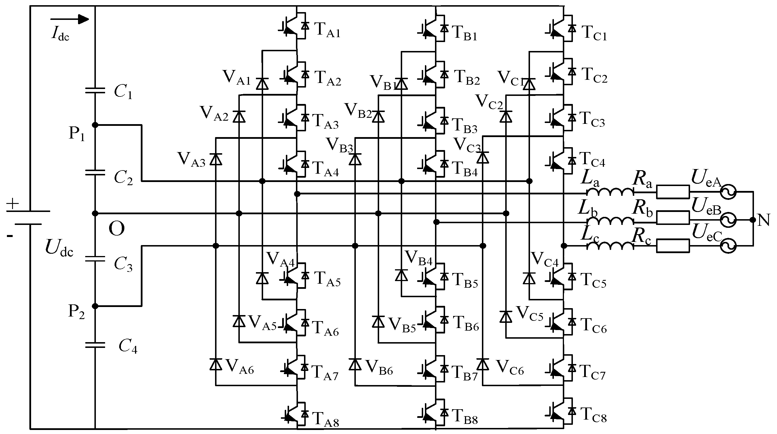
Figure 2.
Comparison of modulation wave and carrier wave.

Figure 3.
The block diagram of the system.

Figure 4.
Simulation of passivity-based control. (a) Phase voltage of the inverter; (b) Line voltage of the inverter; (c) The output function ud; and (d) The output function uq.
Figure 4.
Simulation of passivity-based control. (a) Phase voltage of the inverter; (b) Line voltage of the inverter; (c) The output function ud; and (d) The output function uq.
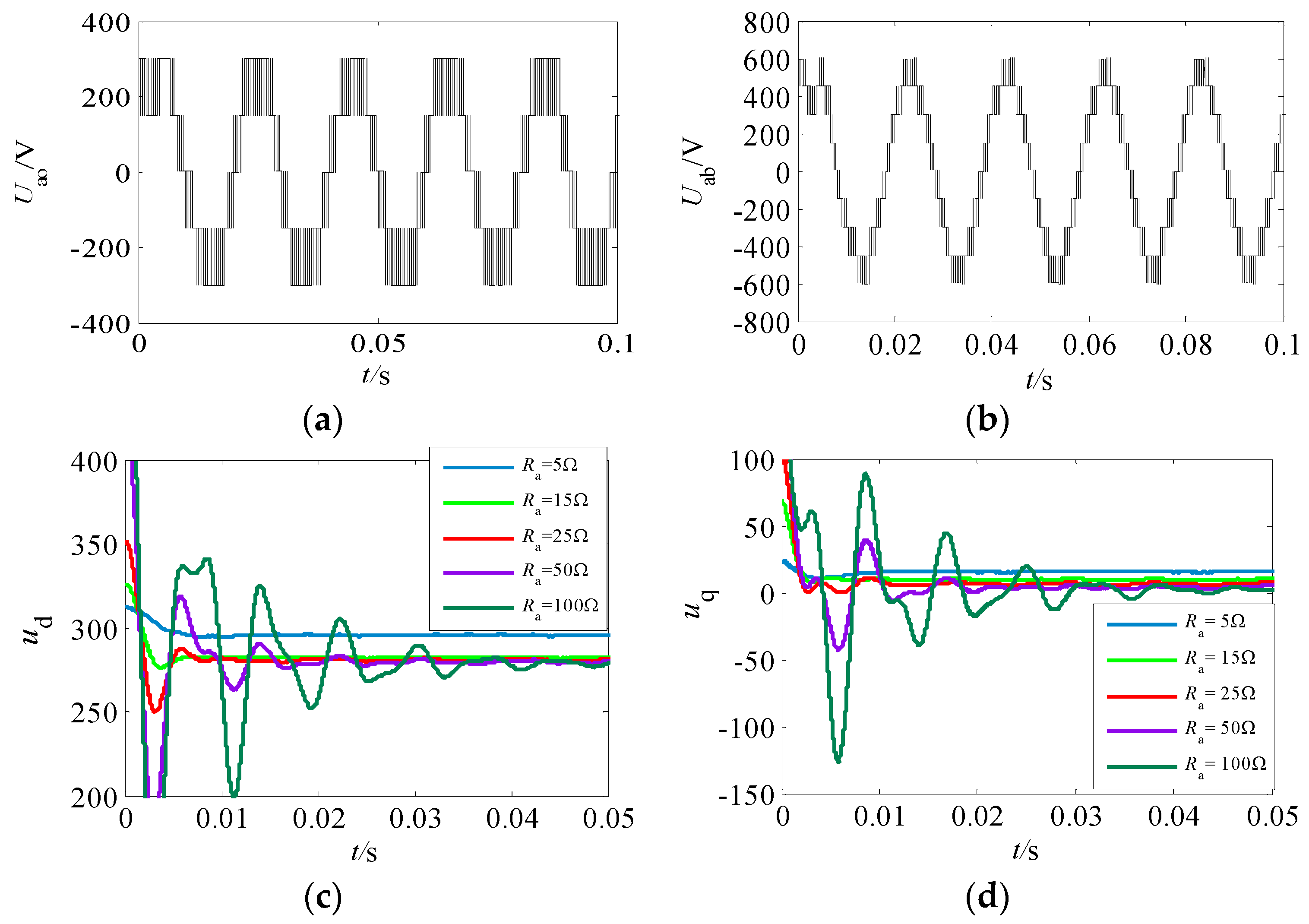
Figure 5.
Comparison of static and dynamic stability under two strategies. (a) The output active power of the inverter under a passivity-based control (PBC) strategy; (b) The output active power of the inverter under the traditional PI control strategy; (c) The d-axis current under a PBC strategy; and (d) The d-axis current under the traditional PI control strategy.
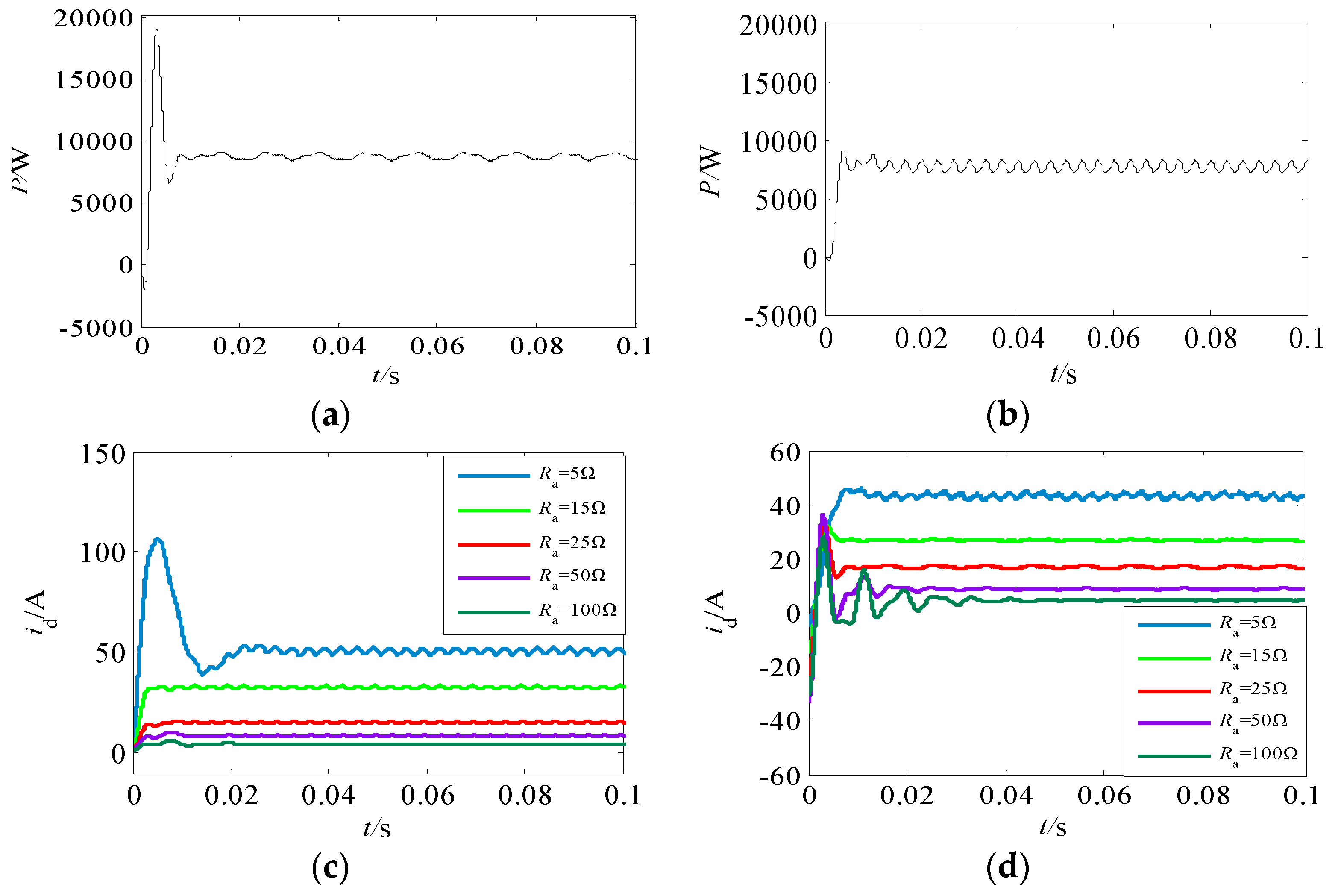
Figure 6.
Comparison of phase and harmonics in two strategies; (a) A-phase grid voltage and current under a passivity-based control strategy; (b) A-phase grid voltage and current under the traditional PI control strategy; (c) A-phase current harmonics of the inverter under a passivity-based control strategy; and (d) A-phase current harmonics of the inverter under the traditional PI control strategy.

Figure 7.
Photo of the hardware experimental platform.
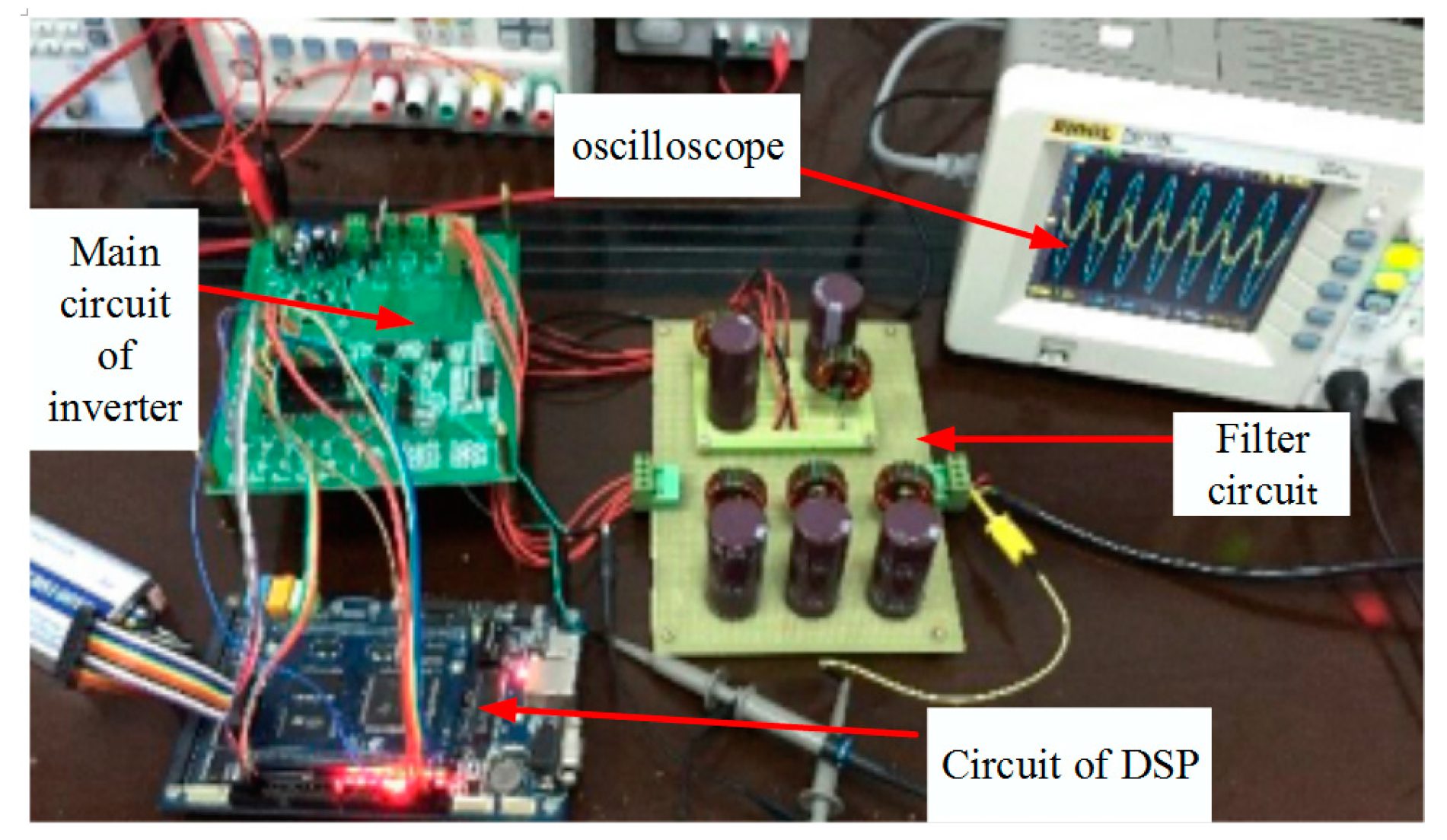
Figure 8.
Comparison of hardware experiments under two strategies; (a) A-phase grid-connected voltage and current under a PBC strategy; (b) A-phase grid-connected voltage and current under the traditional PI control strategy; (c) The d-axis current of different injection dampings under the two control strategies; and (d) The polar film capacitor voltage under a PBC strategy.
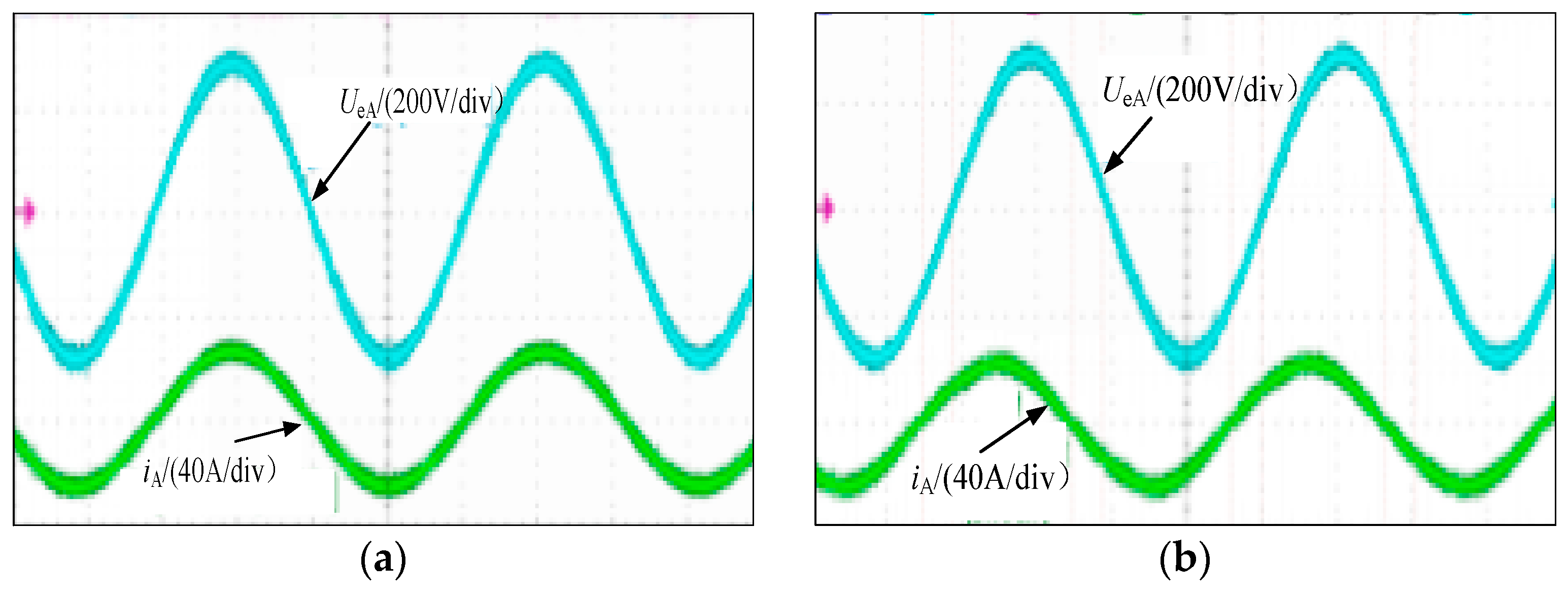
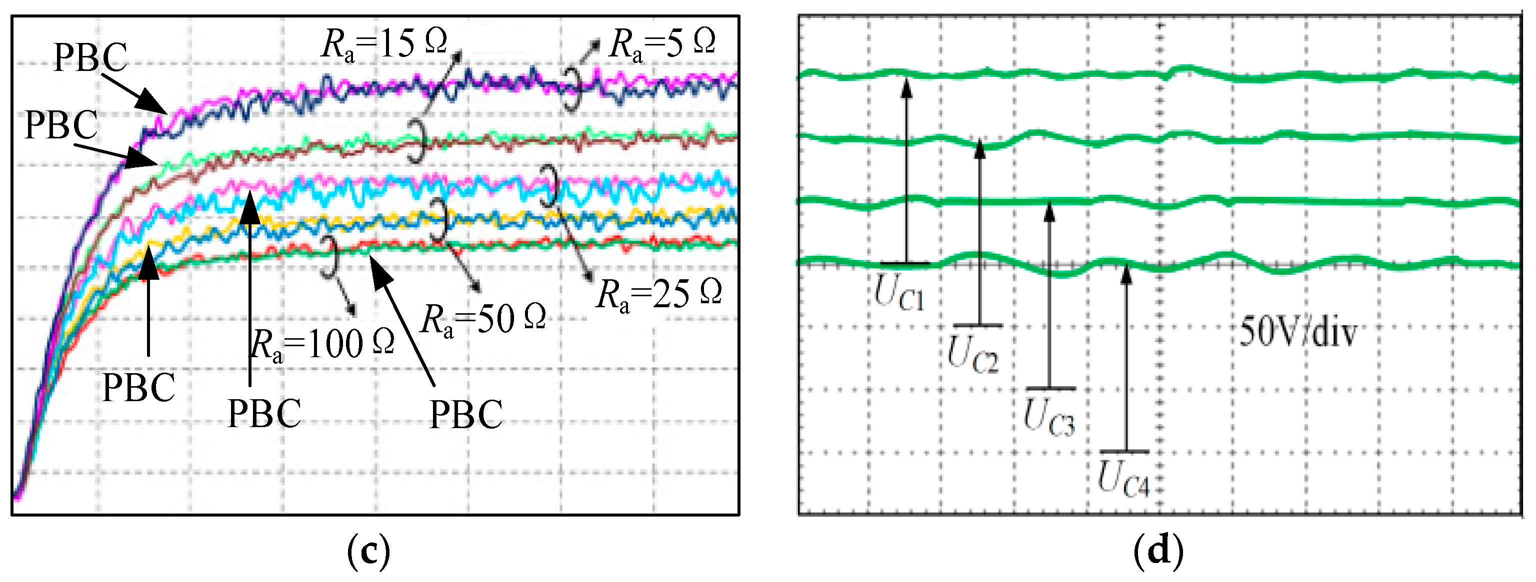
Figure 9.
Phase voltage and line voltage of the inverter; (a) Phase voltage of the inverter; and (b) Line voltage of the inverter.
Figure 9.
Phase voltage and line voltage of the inverter; (a) Phase voltage of the inverter; and (b) Line voltage of the inverter.


Table 1.
Simulation parameters.
| Parameter | Value | Parameter | Value |
|---|---|---|---|
| Udc | 600 V | Lf | 1 mH |
| C1 (C2 C3 C4) | 220 μF | R | 1 Ω |
| C | 50 μF | UeA UeB UeC | 311 V |
| L | 500 mH | frequency (f) | 50 HZ |
Table 2.
Stability time of ud and uq.
| Injection Damping | Stability Time of ud | Stability Time of uq |
|---|---|---|
| Ra = 5 Ω | 0.006 s | 0.005 s |
| Ra = 15 Ω | 0.005 s | 0.005 s |
| Ra = 25 Ω | 0.005 s | 0.006 s |
| Ra = 50 Ω | 0.02 s | 0.02 s |
| Ra = 100 Ω | 0.04 s | 0.045 s |
Table 3.
Comparison of the two control strategies.
| Parameter | PBC | Traditional PI | ||
|---|---|---|---|---|
| Stability Time | Amplitude of Fluctation | Stability Time | Amplitude of Fluctation | |
| p | 0.01 s | smaller | 0.01 s | larger |
| Ra = 5 Ω | 0.02 s | smaller | 0.01 s | larger |
| Ra = 15 Ω | 0.003 s | smaller | 0.01 s | larger |
| Ra = 25 Ω | 0.003 s | smaller | 0.01 s | larger |
| Ra = 50 Ω | 0.004 s | smaller | 0.02 s | smaller |
| Ra = 100 Ω | 0.004 s | smaller | 0.04 s | smaller |
| THD (%) | 0.26 | 3.39 | ||
© 2017 by the authors. Licensee MDPI, Basel, Switzerland. This article is an open access article distributed under the terms and conditions of the Creative Commons Attribution (CC BY) license (http://creativecommons.org/licenses/by/4.0/).
Share and Cite
MDPI and ACS Style
Li, T.; Cheng, Q.; Sun, W.; Chen, L. Grid-Connected Control Strategy of Five-level Inverter Based on Passive E-L Model. Energies 2017, 10, 1657. https://doi.org/10.3390/en10101657
AMA Style
Li T, Cheng Q, Sun W, Chen L. Grid-Connected Control Strategy of Five-level Inverter Based on Passive E-L Model. Energies. 2017; 10(10):1657. https://doi.org/10.3390/en10101657
Chicago/Turabian StyleLi, Tao, Qiming Cheng, Weisha Sun, and Lu Chen. 2017. "Grid-Connected Control Strategy of Five-level Inverter Based on Passive E-L Model" Energies 10, no. 10: 1657. https://doi.org/10.3390/en10101657
Note that from the first issue of 2016, this journal uses article numbers instead of page numbers. See further details here.