High Voltage Overhead Power Line Routing under an Objective Observability Criterion

Abstract

The construction of new high voltage overhead power lines (HVOPLs) has become a controversial issue for electricity companies due to social opposition. Citizens are concerned about how these power lines may have an impact on their lives, basically caused by their effects on health and safety. Visual impact is one of the most easily perceived. Although there are several published works that deal with the assessment of the visual impact produced by HVOPLs, no methodology has been proposed to assess this impact from an objective perspective. This work presents an original methodology which helps to identify the optimal routes for a new HVOPL under an objective observability criterion, enabling the selection of those with the lowest visibility in a zone. The application of the proposed methodology achieves a set of routes that links new HVOPL origin and destination points creating a corridor which includes all possible routes with an observability of its towers under a threshold limit. This methodology is illustrated by a real-life use corresponding to the selection of the route with least observability for a new power line in La Rioja (Spain). The results obtained may help to achieve a consensus between key stakeholders since it is focused on the specific issues of the planned HVOPL and its observability from an objective perspective.

1. Introduction

Electric energy is an essential component in present societies. An inexpensive and reliable electrical supply is a precondition for a competitive economy and, thus, an important basis for our technological society. In the design of new power infrastructures, it is important to consider the psychological aspects of how our culture considers and accepts its development as an integral component of the community’s physical environment [1].

The construction of new high voltage overhead power lines (HVOPLs) in rural areas is the one of the most adopted solutions adopted to integrate medium and large size power plants based on renewable sources into the grids. Whereas this integration is widely accepted, the general acceptance of energy projects is higher than local acceptance [2].

The kind of impact that HVOPLs can have on population can be divided into environmental and visual. Environmental impact include life cycle impact, impact on vegetation and wildlife, and electromagnetic impact. Visual impact, which is related to visibility and aesthetic aspects, differs from one person to another, but it generally depends on the landscape, position and angle of the observer, as well as the contrast [3]. Visual impact itself constitutes one of the objections raised by communities who oppose the construction of new power lines [4]. In some works, visibility has been used as an indicator of visual impact, but visibility and visual impact are not equivalent terms: visibility refers to the ability to discern an object from its surrounding landscape while visual impact takes into account the sociocultural attributes of the viewers resulting in the perception of visual aesthetic impact [5]. Anyway, visibility and proximity play a key role for visual impact assessments. For example, in some new HVOPL projects, the perceived health and safety effects have been considered to be more important than visual impact, but the visibility and proximity of the new HVOPL increase the sense of threat for health and safety [6].

The Landscape and Visual Impact Assessment (LVIA) technique is widely used to assess the effects of change on the landscape that can be caused by human intervention [7]. Recently, visual impacts produced by different power components have been further studied in literature, mainly those caused by power plants based on renewable energies such as wind farms [8,9,10,11], photovoltaic plants [9,10,12] and small hydro plants [9]. Even, for PV systems, objective and quantitative methods have been developed for evaluating the visual impact [13,14]. However, compared with other power infrastructures in the landscape, there has been relatively little research on the perceptions of power transmission lines [15].

The visual impact caused by new HVOPLs has been discussed by Harrison [16]. This author defines “visual disamenity cost” as a measure to assess the visual impact of an HVOPL and identifies the factors concerning tower design and location, which may affect the visual impact of these lines (tower height, tower location, colour, tower construction and extent of screening by vegetation). Some studies, such as [17], have found that the social benefits of avoiding the negative aesthetic impact on the landscape of HVOPLs in an urban setting exceed the costs of burying the line as underground cables. This is so even though in rural areas the larger costs for underground cables, with respect to those of HVOPLs, makes this strategy possible only in zones of relevant environmental interest [18]. Surveys and questionnaires have been widely used to assess the impacts, including the visual impact, on the population living in the zone where a new power line is being projected [15,18,19,20].

Visual impact is one of the causes that promotes local opposition to the construction of new HVOPLs. The erection of a new infrastructure perceived by population as imposed, especially if it changes the landscape, increases social opposition [21]. The construction of new projects can be blocked, or at least delayed, by the opposition of local population, causing enormous costs to the utilities [22], with discussions between local residents, network operators and other stakeholders usually taking place at an emotional level [23]. This opposition has caused network operators to opt for optimizing the existing network by renewing outdated HVOPLs rather than constructing new ones [24]. The selection of routes with the lowest visibility on a zone can contribute to reducing oppositions and accelerating the construction of new HVOPLs.

Geographic information systems (GISs), software technologies developed for spatial data analysis, are suitable tools for such selection. GISs allow the simultaneous evaluation of key technical, economic and environmental factors. GISs were identified as the ideal equipment to use quantitative methods in environmental assessment [25,26] and they have been used in visual impact assessment [27,28]. GISs handle data in digital models; raster data model is one of the most useful. Raster data model divides the geographic area into a grid of georeferenced cells. These cells can store the values of a variable of interest.

Warner [29] presents the use of a GIS in an environmental impact assessment of an HVOPL: the visual impact is included as one of the criteria, but considering only the visibility of the selected routes within a distance of 3 km from a mountain zone with scenic beauty and touristic interest. The Electric Power Research Institute and the Georgia Transmission Corporation (EPRI-GTC) developed the Overhead Electric Transmission Line Siting Methodology [30] that deals with visual impact creating a “visual exposure map”, which is a grid-based map (raster map) where each cell value represents the number of times a location is seen from a set of viewer locations (mainly houses or roads). In the case of roads, each cell crossed by a road constitutes a viewer location for the visual exposure map. The values stored in this map do not take directly into account the number of inhabitants (houses) or travellers (roads). The methodology can be used to compare alternative routes, but it does not provide the optimal route under visual impact criteria. Erdmann [23] proposes a transparent and objective method to assess the visibility of the towers of a HVOPL over predefined routes. Grassi [31] presents a new methodology followed to calculate suitable routes for new power lines. The methodology takes into account visual impacts caused by cables or masts as one of the six different criteria (topographic, terrain, linear infrastructures, danger areas, protected areas and visibility). Viewer locations are restricted to buildings. Corridors are identified in the global cost map (defined with the six criteria) as the areas covered by, at least, one of the optimal routes obtained by applying different weighting factors to each criterion.

This article presents a new methodology for objectively determining possible routes for a new HVOPL with a defined limit for the visibility or observability of its towers. This methodology is based on GIS and allows to obtain a map to identify visual corridors. This map is called the Corridor Selection Map (CSM). We define visual corridors as the areas in the CSM where the cumulative cost of the path from an origin cell to a destination cell and crossing any cell of the area lies below a certain threshold. The variable used as cost is the Global Potential Observation Hours (GPOH), which is defined in the methodology section. Visual corridors are areas that include the optimum and near optimum routes under the observability criterion; for each cell within a visual corridor a route can be traced crossing that cell and with a cumulative value for the GPOH variable under a defined limit.

The CSM with the visual corridors obtained through the application of the methodology proposed can be integrated with others obtained under other criteria (environmental, economic, etc.) and can help to achieve a consensus between key stakeholders since it is focused on the specific issues of the planned transmission line and its observability under an objective perspective.

The article is structured as follows: Section 2 presents the methodology proposed for the optimal route selection of a new HVOPL. Section 3 shows the application of this methodology to a real-life case considering a 66 kV HVOPL crossing a rural zone in La Rioja (Spain). Finally, Section 4 presents the conclusions.

2. Proposed Methodology

The methodology proposed creates a GIS map, the CSM, which helps to find possible paths in a zone for a new HVOPL under an objective observability criterion. The CSM is obtained from other two maps containing the Lowest Cost Paths (LCPs), as it is explained in Section 2.2. We define a LCPs map as a raster file which contains in each cell the minimum accumulated cost value following the optimal path from an origin, defined by the user, to that cell. The optimal path corresponds to the route with the minimum accumulated cost. The variable used as cost is the Global Potential Observation Hours (GPOH), which corresponds to the cumulative value of the number of hours in a mean day in which any tower of the new HVOPL can be viewed by all the possible observers. The GPOH depends on the orography of the zone where the new line is going to be built, the possible observers (inhabitants or travellers), and their position with respect to the towers of the new HVOPL. The evaluation of the GPOH variable for all raster cells allows obtaining the Global Potential Observation Hours Map (GPOHM) which represents a geographical zone where to identify the areas with higher or lower observability for the new HVOPL. The evaluation also enables to choose the route with the lowest observability and, therefore, with the lowest visual impact in the zone.

The variable GPOH corresponds to the sum of variable Potential Observations Hours (POH) for all the possible observer positions. We define the POH variable for a single observation point (village, farm, etc.) or for a single segment (of road, railway, etc.) as a numerical value that mainly takes into account the number of potential observers. Since human visual acuity diminishes with distance [32], the distance between the potential observer and the observed object acts as a weighting factor of the number of potential observers in order to calculate the POH value. This value also depends on the orography of the geographic area where observers and observed object are placed.

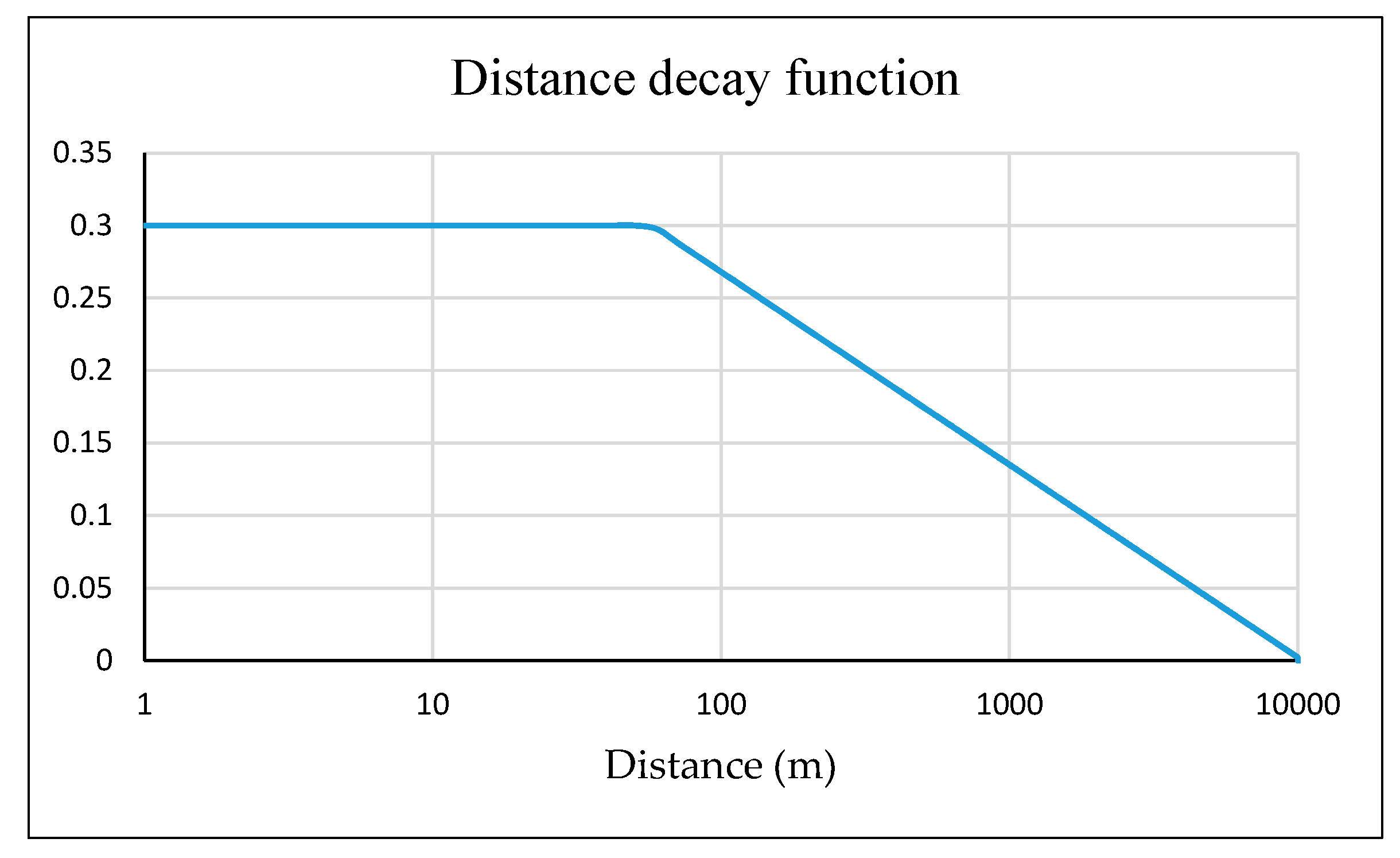
Some GIS-based methodologies have been proposed in literature to consider the distance from the observer to the observed object. The most popular is the fuzzy viewshed method proposed by Fisher [33]. The author proposes the use of fuzzy membership functions, whose values decrease with the distance. In the methodology presented in this paper we have used a similar approach using a weighting function. The parameters of this weighting function were adjusted taking into account the height of the power line towers structure and the limit of human recognition acuity. This function, whose values decline with distance, was proposed in [34] and is shown in (1):

$$\{\begin{array}{l}w=0.3\mathrm{for}d\le 57.5\mathrm{m}\hfill \\ w=\frac{-0.0638·\ln (d)+0.59}{1.105}\mathrm{for}57.5<d<\mathrm{10,000}\mathrm{m}\hfill \\ w=0\mathrm{for}d\ge \mathrm{10,000}\mathrm{m}\hfill \end{array}$$

(1)

where w represents the weighting factor and d is the distance between the positions of the observer and of the observed object (power line tower). Figure 1 plots this weighting function. The orography of the terrain between the potential observers and the HVOPL plays a key role in the calculation of the POH values. For example, a power line tower cannot be seen from some near areas in a zone due to orographic accidents (hills, depressions, etc.). In order to take into account the orography, we use the Digital Terrain Model (DTM), that is, a raster file representing the terrain of the zone under study. The cell size is chosen according to the average span length of the electric line (one cell, one tower).

2.1. The Global Potential Observation Hours Map (GPOHM)

The calculation of the GPOHM is done differently for observers with a static position (on-site observers) and for observers in motion (on-road observers). We consider the same height above the ground for the towers of the new HVOPL in both cases.

2.1.1. On-Site Observers

The process starts with the creation of a table in which all the necessary information is stored (on-site observers table). This information corresponds, for each observation point, to its geographic position, the number of potential observers and their height above the ground in that point. Depending on the characteristic of the on-site point, the number of potential observers can correspond to inhabitants (communities, isolated houses, farms, etc.), or to daily visitor (viewpoints, monuments, etc.). Suppose an observation point j and a tower of the new HVOPL placed in the area represented by cell i, the value of the POH variable considering only the point j and the cell i, POH_i,j, is calculated as follows:

• The data corresponding to point j is read from the on-site observers table.
• The visibility of the tower placed in the area represented by cell i is determined with the application of a filter: the filter returns a value, f_i,j, equal to “1” if the tower is visible from the observation point j (taking into account the height of the tower and the height above the ground of the observers in point j). The value f_i,j is “0” if the tower is not visible form point j. This filter is a predefined GIS function.
• The Euclidean distance, d_i,j, from the central point of the area represented by cell i to the point j is obtained using GIS functions.
• The weighting factor, w(d_i,j), corresponding to distance d_i,j is calculated by means of (1).
• The POH_i,j value is calculated as the product of the value provided by the filter (f_i,j), the number of observers in point j (obs_j), the weighting factor, w(d_i,j), and the number of daylight hours in a mean day (hmd), as expressed by (2):

  $$PO{H}_{i,j}=f_{i,j}·ob{s}_j·w\left(d_{i,j}\right)·hmd$$

  (2)

This procedure is followed for all the observation points and the values aggregated to obtain the On-Site Global Potential Observation Hours value for a tower placed in the area represented by cell i, OSGPOH_i. Supposing a total of J on-site observation points, this value is calculated by means of (3), and its result stored in the cell i:

$$OSGPO{H}_i={\displaystyle \sum _{j=1}^{J}PO{H}_{i,j}}$$

(3)

2.1.2. On-Road Observers

For on-road observers, they are travelling along a road, what makes different the calculation process. The number of possible observers is evaluated using the average daily traffic (ADT), which corresponds to the average number of vehicles per day. The ADT values can be obtained from local authorities which can provide a different ADT value for each road stretch. A road stretch is limited by two bifurcations or crosses. We divide the road stretches into road segments which are the portions of a road stretch with the same average speed for the vehicles.

A new table, the on-road observers table, is created to store the necessary information. This table contains, for each road segment, the ADT value, its length, the average speed and the average height above the ground of travellers in a vehicle. The tower height is the same that the used for on-site observers.

In order to identify observation points from a road segment, we divide it into evenly separated nodes. The length between consecutive nodes divided by the average speed represents the observation time, t_n, in a node (the faster speed, the lower watching time). Suppose a road segment k and a tower of the new HVOPL placed in the area represented by cell i, the value of the POH variable considering only the road segment k and the cell i, POH_i,k, is calculated as follows:

• The data corresponding to road segment k is read from the on-road observers table. The road segment is divided into nodes.
• For each node, n, in road segment k:
  • A filter is applied: the filters returns a value, f_i,n, equal to “1” if the tower placed in the area represented by cell i can be seen from the geographic position corresponding to the node n, otherwise it returns a value “0”. The height of the HVOPL tower and the average height above the ground of travellers are taken into account in the application of this filter.
  • The Euclidean distance, d_i,n, between the node n and the central point of the area represented by cell i is obtained using GIS functions.
  • The weighting factor corresponding to distance d_i,n is calculated by means of (1).
  • The product of the value obtained with the filter, f_i,n, the weighting factor, w(d_i,n), and the observation time in node n, t_n, is accumulated in cell i.
• After processing all the nodes of road segment k, N_k, the value accumulated in cell i is converted to POH_i,k value multiplying it by the ADT of road segment k, ADT_k, and the average number of persons per vehicle in that road segment, obs_k, as expressed in (4):

  $$PO{H}_{i,k}=AD{T}_k·ob{s}_k·{\displaystyle \sum _{n=1}^{N_k}{f}_{i,n}·w\left(d_{i,n}\right)·t_n}$$

  (4)

The procedure is repeated for all the road segments in the zone under study, a total of K road segments. The aggregation of the POH_i,k values obtained for each road segment, as expressed in (5), allow us to calculate the On-Road Global Potential Observation Hours value, ORGPOH_i, which represents the aggregated number of hours in a mean day in which the HVOPL tower placed in the area represented by cell i can be seen by on-road observers.

$$ORGPO{H}_i={\displaystyle \sum _{k=1}^{K}PO{H}_{i,k}}$$

(5)

Although we have presented the procedure to take into account travellers in a vehicle, it can be easily modified to study other kind of travellers (in train, pedestrians, in bicycle, etc.). All it needs is to include new rows reflecting the data information for these new kind of travellers.

2.1.3. Global Potential Observability Hours Map (GPOHM)

Finally, the Global Potential Observability Hours (GPOH) value for each cell i can be calculated by aggregating the values of the OSGPOH_i and ORGPOH_i. In this aggregation two factors, ${\lambda }_1$ and ${\lambda }_2$, can be considered in order to assign different importance for on-site or on-road observers (6).

$$GPO{H}_i={\lambda }_1·OSGPO{H}_i+{\lambda }_2·ORGPO{H}_i$$

(6)

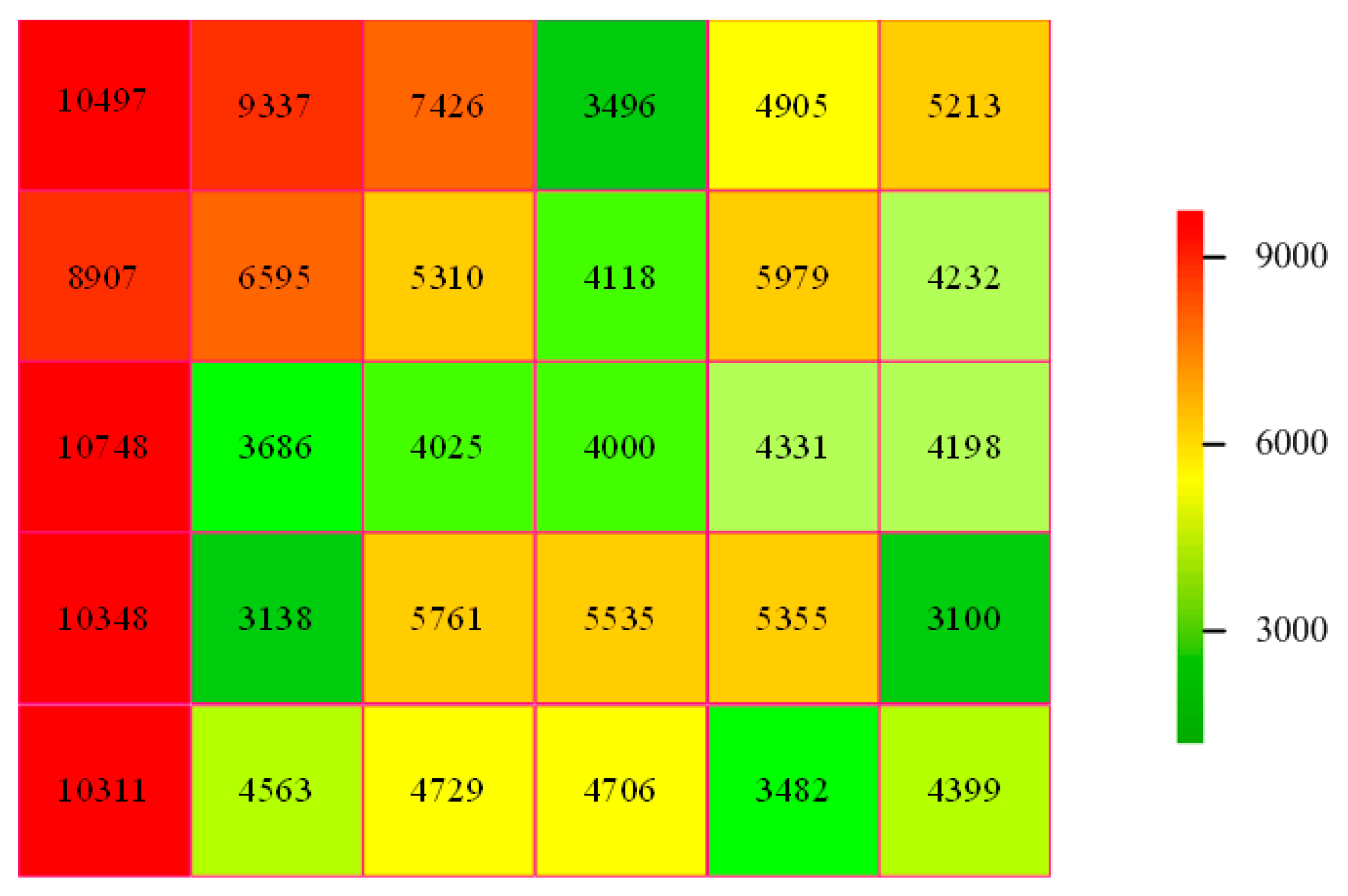
After obtaining GPOH_i values for all the cells, they can be represented in a map, the GPOHM. Figure 2 shows an example of a GPOHM section.

2.2. HVOPL Routing under the Observability Criterion

2.2.1. Lowest Cost Paths (LCPs)

Our starting point is the GPOHM previously obtained. The selection of the neighbouring cells linking an origin and a destination point constitutes the base of line routing in a GIS raster file. The optimal path between two cells, representing different geographical positions in the map, is the set of cells optimally linked to their neighbouring cells in a sequential manner along the route.

The calculation is based on the application of the package gdistance [35], implanted in the R software [36], which provides functions to calculate various distance measures and routes in heterogeneous geographic spaces represented as grids or raster files.

The GPOHM is a map which represents a two-dimensional space Ω = {(x, y): x = 0, …, X; y = 0, …, Y}, where the elementary (x, y) cell is a geographic location where a HVOPL tower can be erected. The set P = {p₀,…, p_k,…, p_K} = {(x₀, y₀),…, (x_k, y_k),…,(x_K, y_K)} = segments{s₁,…, s_k,…, s_K} is the route composed of K + 1 cells (and towers). Line segments s_k are the links between cells p_k-1 and p_k. A segment can only link neighbouring cells in space Ω, that is, from one cell to one of the eight neighbouring cells Ω (p_k)$\in$(1...8).

A transition value is associated with each segment linking two neighbouring cells p_k-1 and p_k. This value is independent of the direction followed by the segment, that is, in our study the transition value is just the GPOH value stored in cell p_k, as expressed in (7):

$$f(s_k)=GPO{H}_{p_k}$$

(7)

The optimal route from the origin cell to any destination cell is the set P (set of segments) which correspond to the lowest accumulated transition values. LCPs map corresponds to the raster file where the lowest accumulated transition values from the origin cell are stored in each cell. In order to take into account the value of GPOH variable in the origin cell (first tower of the HVOPL), that value is added to all the cells in that map, obtaining the LCPs map. 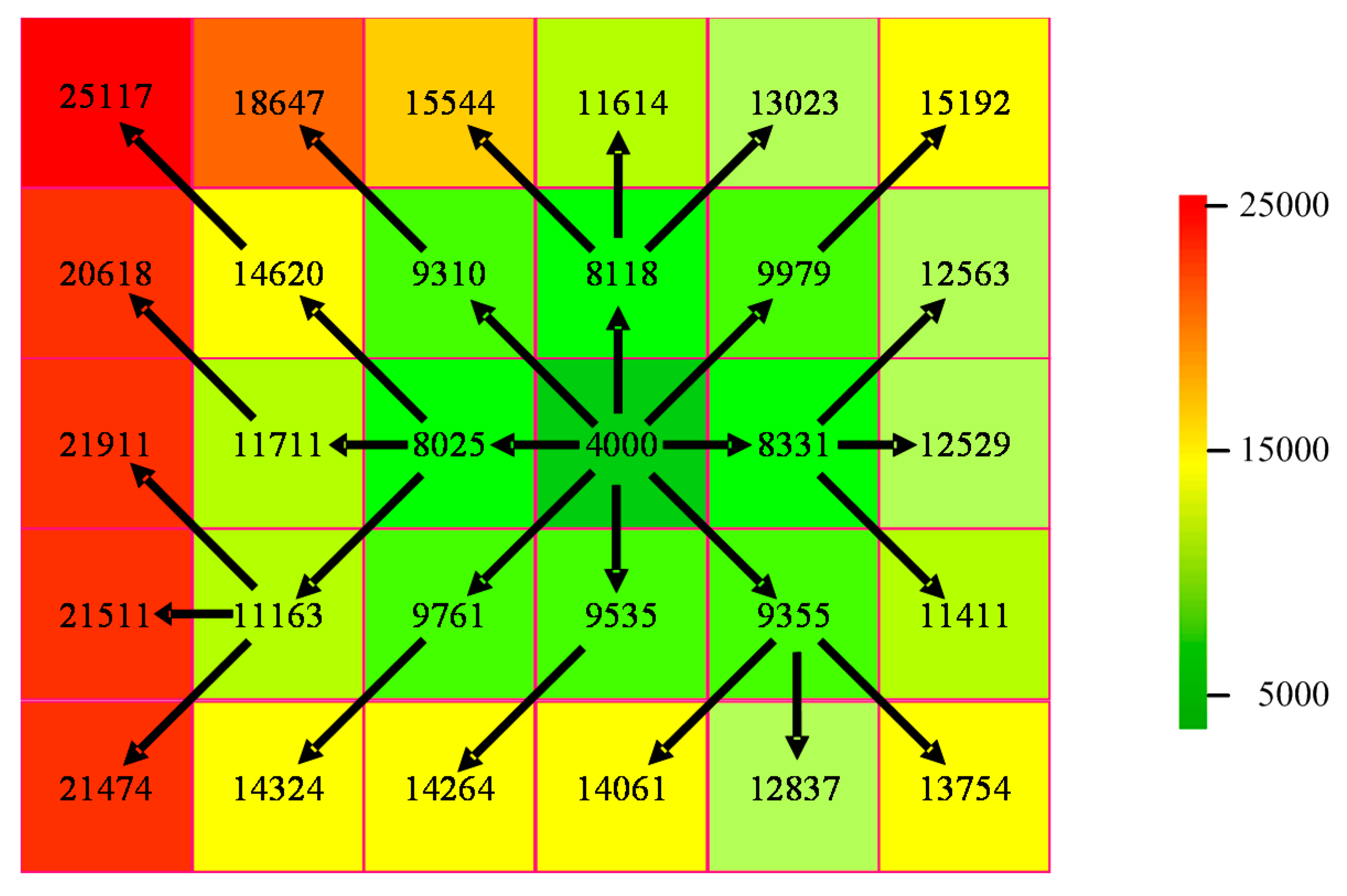Figure 3 shows a section of a LCPs map obtained taking the cell in dark green as origin cell and using the GPOHM represented in Figure 2. The value contained in each cell of the map in Figure 3 corresponds to the accumulated value of the GPOH following the optimal route from the origin. The arrows indicate the selected links between neighbouring cells in the computation process.

2.2.2. Corridor Selection Map (CSM)

The CSM is obtained by computing two LCPs maps previously: the first one is obtained by taking the origin of the HVOPL as the origin cell (cell A), and the second one is obtained by taking the destination of the HVOPL as the origin cell (cell B). By adding the value of the two LCPs maps in each cell together and subtracting the value of the GOPHM, we obtain the CSM value for each cell, as indicated in (8):

$$CS{M}_{p_k}=LCP{s}_{A,p_k}+LCP{s}_{B,p_k}-GPO{H}_{p_k}$$

(8)

Since value LCPs_A,pk corresponds to the cost (in GPOH) of the optimal path from origin A to the area represented by cell p_k, and LCPs_B,pk corresponds to the cost of the optimal path from destination B to the area represented by cell p_k, then the addition of the two values together, for each cell, gives the cost of the optimal path that links the origin and destination crossing that cell. We need to subtract the GPOH value, as it is computed in both LCPs maps.

Visual corridors are defined within boundary regions in the CSM, as the set of cells with a value, $CS{M}_{p_k}$, lower than a threshold value (h_max) defined by the user:

$$p_k\in \mathrm{\Omega },:CS{M}_{p_k}\le h_{\max }$$

(9)

The optimal path is composed by all the cells containing the minimum value, h_min. On the other hand, the cells containing the threshold value, h_max, belong to the bounds of the corridor. Therefore, visual corridors are areas inclosing optimum or near optimum paths under the observability criterion. The visual corridor bounds are composed by the cells which value corresponds to the threshold selected by user.

3. Case Study

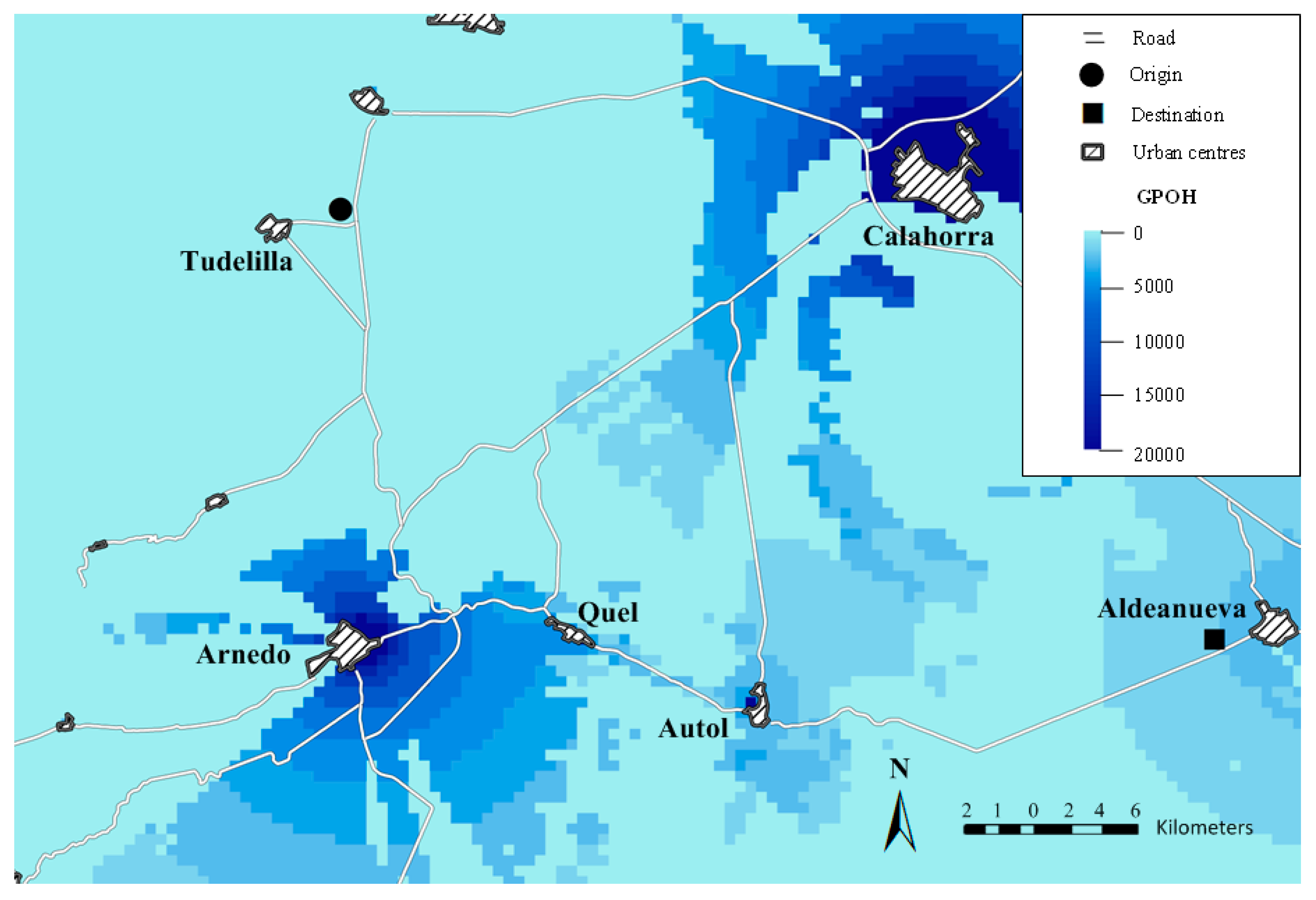
We present a case study for a zone located at the southeast of La Rioja (Spain). In the case we study the installation of a new 66 kV HVOPL from an origin location (near the town centre of Tudelilla) to a destination location (near the town centre of Aldeanueva) in La Rioja, a wine region that it is promoting the tourism industry with its vineyards landscape as a claim. The relative positions of the origin and destination points of the planned HVOPL are presented in Figure 4.

The proposed methodology was applied to the zone under study. This zone includes 22 on-site observation points (urban centres, villages and hamlets) and 53 road stretches. Since the urban centres in the geographic zone of this case study are relatively small, for each urban centre we considered the number of observers equal to its number of inhabitants and we placed the observation point in its centroid. Moreover, most of the road stretches have only one speed limit for vehicles which is related to the road type (highway, local or national road), we considered that the number of road segments was 53. The distance between consecutive nodes in the road segments was fixed in 1 m. The traffic measurement stations were considered to obtain the ADT value for daylight hours.

The main communities in the area under study are the towns of Arnedo (14,551 inhabitants), Quel (2027 inhabitants) and Autol (4367 inhabitants), all of them located in the centre of the area, and the town of Calahorra (24,202 inhabitants), northwards. The roads linking the town centres are coloured in white in the map of Figure 4.

The computational process was carried out to identify the visual corridors, following the observability criterion, corresponding to the construction of the new HVOPL. The planned HVOPL is expected to have towers of 25 m high spanned every 200–300 m long. A GIS cell size of 200 × 200 m was selected so that each cell represents a potential area for the erection of one of the towers. The DTM with the desired resolution and the geographic information data related to the roads in the zone under study, were downloaded from the geographic data server of the Ministry of Public Works and Transport of Spain [37]. We used a value of 1.72 for the average number of persons per vehicle in all the road segments in the zone under study, according to the latest available statistical data referred to Spain [38]. We used ${\lambda }_1={\lambda }_2=1$ for the two factors in (6), that is, we assigned the same importance to both type of observers (on-site and on-road).

The methodology described in Section 2 was implemented to obtain the GPOHM for the area under study. Figure 4 shows the GPOHM obtained, where the contribution of on-site observers can be identified as larger than that of on-road observers (dark colours, corresponding to higher values of GPOH, near centres with more inhabitants). The light colours represent the cells with low values of GPOH. As it is shown, areas surrounding the main town centres present the highest values of GPOH, although there are near areas with low values because they cannot be seen due to orographic obstacles. It is important to notice the effect of these obstacles on GPOH near Arnedo and Calahorra (e.g., the zone to the south of Calahorra cannot be seen by its inhabitants because it is on a plateau higher than the town centre). In Figure 4, dark colours represent the higher values which correspond to areas that can be seen by most of the potential observers.

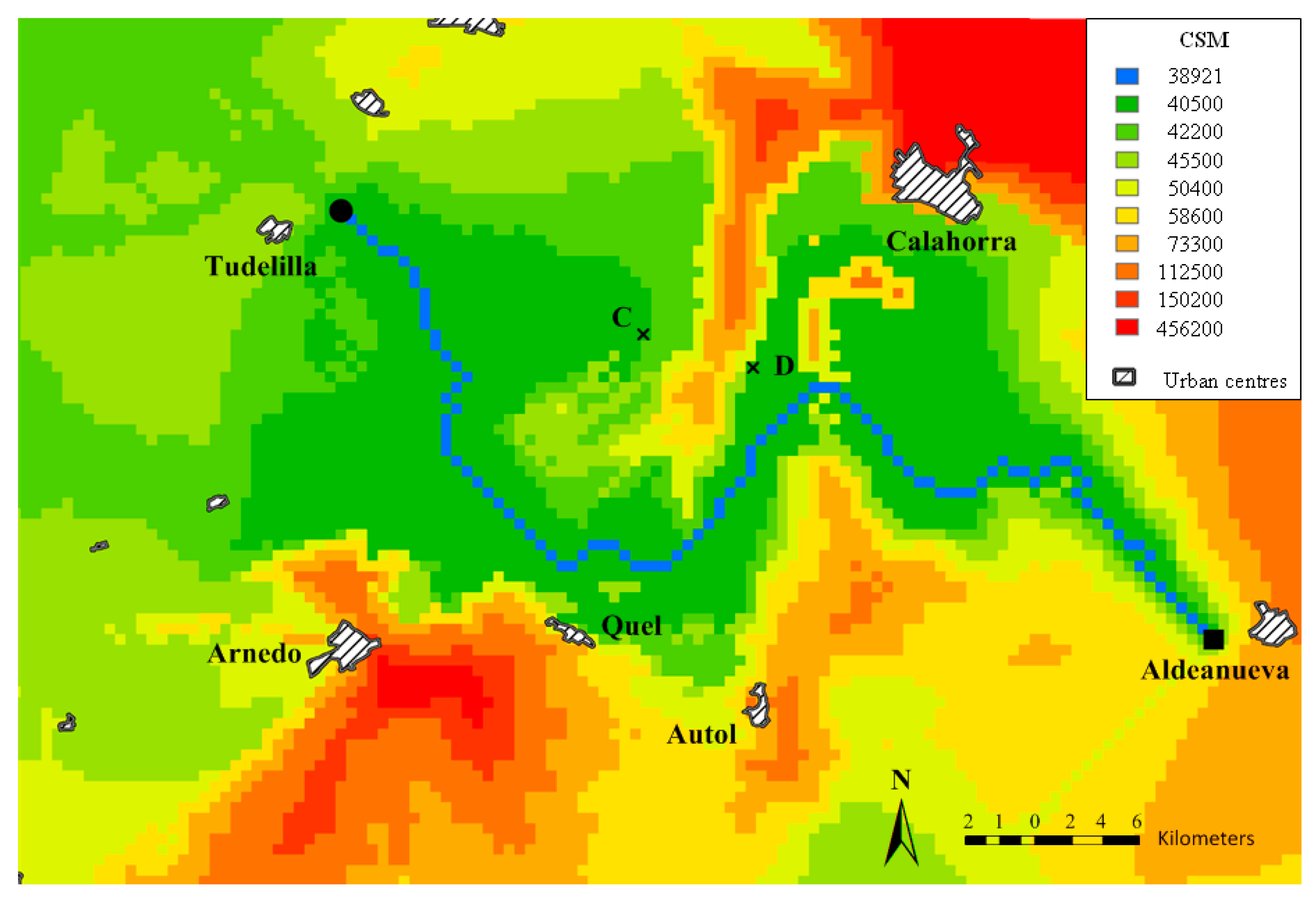
LCPs maps from the origin and destination of the planned HVOPL were calculated, as described in Section 2.2, and the CSM was obtained according to (8). The value in each cell of this map (whose values are hours) represents the minimum accumulated observability hours for a HVOPL, with the previously defined characteristics, passing through such cell and linking origin and destination. Figure 5 shows the calculated CSM. The optimal path for the HVOPL (minimum observability of its towers) that links the origin and destination is formed by the cells of that map coloured in blue colour, which have the same and minimum value in this map (h_min = 38,921 h). This value represents an objective quantity of the observability of the proposed 66 kV HVOPL. The value in the rest of the cells of this map is greater than h_min and its difference with respect to h_min represents the “distance” in terms of visibility between the optimal path that passes through that cell and the optimal path between origin and destination without the restriction of passing through such a cell.

We define different threshold values (h_max = 40,500, 42,200, 45,500, 50,400, 58,600, 73,300, 112,500, 150,200 and 456,200 h) in the CSM to obtain different visual corridors. These threshold values were selected as an illustrative example. Inside each corridor several different routes can be selected with a value of accumulated observability hours lower than the h_max value, which defines the bounds of such corridor. Furthermore, visual corridors in Figure 5 can help to identify the areas (cells) where is preferable to transform the planned HVOPL into an underground one under the observability criterion if burying all the power line cannot be considered. For example, if the section of the planned power line between points C and D is constructed as a buried power line (crossing areas with high values of GPOH, but with null observability since it is underground), and the sections between origin and C and between D and destination as an overhead power line, the observability of the whole line would be below the 40,500 h.

The observability criterion used in the proposed methodology can be included as an additional criterion in multi-criteria HVOPL routing systems which include other economic, environmental, or social criteria, enabling to obtain suitable solutions to the automatic selection of line routing with the minimum public opposition.

4. Conclusions

The construction of new HVOPLs is essential to be provided with a reliable electric power supply and facilitate the integration of power plants based on renewable energies. However, this construction is not exempt from social opposition, mainly from inhabitants in the zone where the new line is going to be erected. One of the arguments most used by opponents to the construction of the new HVOPL is visual impact. Since visual impact is subjective, many HVOPL projects try to assess it by means of surveys and questionnaires filled by selected groups of the local population, although this solution does not eradicate the opposition.

This article presents a useful methodology, based on GIS, which allows the selection of the route for a new HVOPL with the lowest visibility in a zone. The methodology achieves the identification of visual corridors in an objective manner. Visual corridors consist of geographical zones that connect the origin and the destination and represent areas where all the towers of the power line can be erected so that the observability of all the line is under a defined threshold limit. The variable used to assess the observability of the HVOPL is the Global Potential Observation Hours, that is, the aggregated number of hours in a mean day in which any tower of a HVOPL can be viewed by all possible observers. All kind of observers, inhabitants and travellers, are taken into account via a quantitative approach. The original solution adopted for on-road observers consists of decomposing the road into segments and determining, with great accuracy, the total amount of time during which any of the towers of the new line can be seen as they travel.

Although in the case study we have considered all the possible observers, all with the same affection level with respect to the landscape (for the objective approach), the proposed methodology could be used assigning different factors to each type of observers according to these levels. For example, it would be possible to change the number of observers in each observation point or road segment, using higher factors for tourists than for local residents.

The use of the proposed methodology offers objective results. All the data needed are the digital terrain model of the zone where the line is going to be erected, the position of the observation points (villages, hamlets, viewpoints, roads, etc.), the number of observers and those related to their motion. The results, in the form of maps, allow the easy identification of different alternatives for the route with greater or lower observability for the towers of the power line. These maps can lead to a consensus among the agents (utilities, local authorities and inhabitants) involved in the construction of the new HVOPL and thus contribute to reducing opposition and accelerating its construction.