Condition Monitoring for Roller Bearings of Wind Turbines Based on Health Evaluation under Variable Operating States


1
The State Key Lab of Fluid Power and Mechatronic Systems, College of Mechanical Engineering, Zhejiang University, Hangzhou 310027, China
2
Key Laboratory of Advanced Manufacturing Technology of Zhejiang Province, College of Mechanical Engineering, Zhejiang University, Hangzhou 310027, China
3
Faculty of Mechanical Engineering and Mechanics, Ningbo University, Ningbo 315211, China
*
Author to whom correspondence should be addressed.
Energies 2017, 10(10), 1564; https://doi.org/10.3390/en10101564
Submission received: 2 August 2017
/
Revised: 20 September 2017
/
Accepted: 28 September 2017
/
Published: 11 October 2017
Abstract
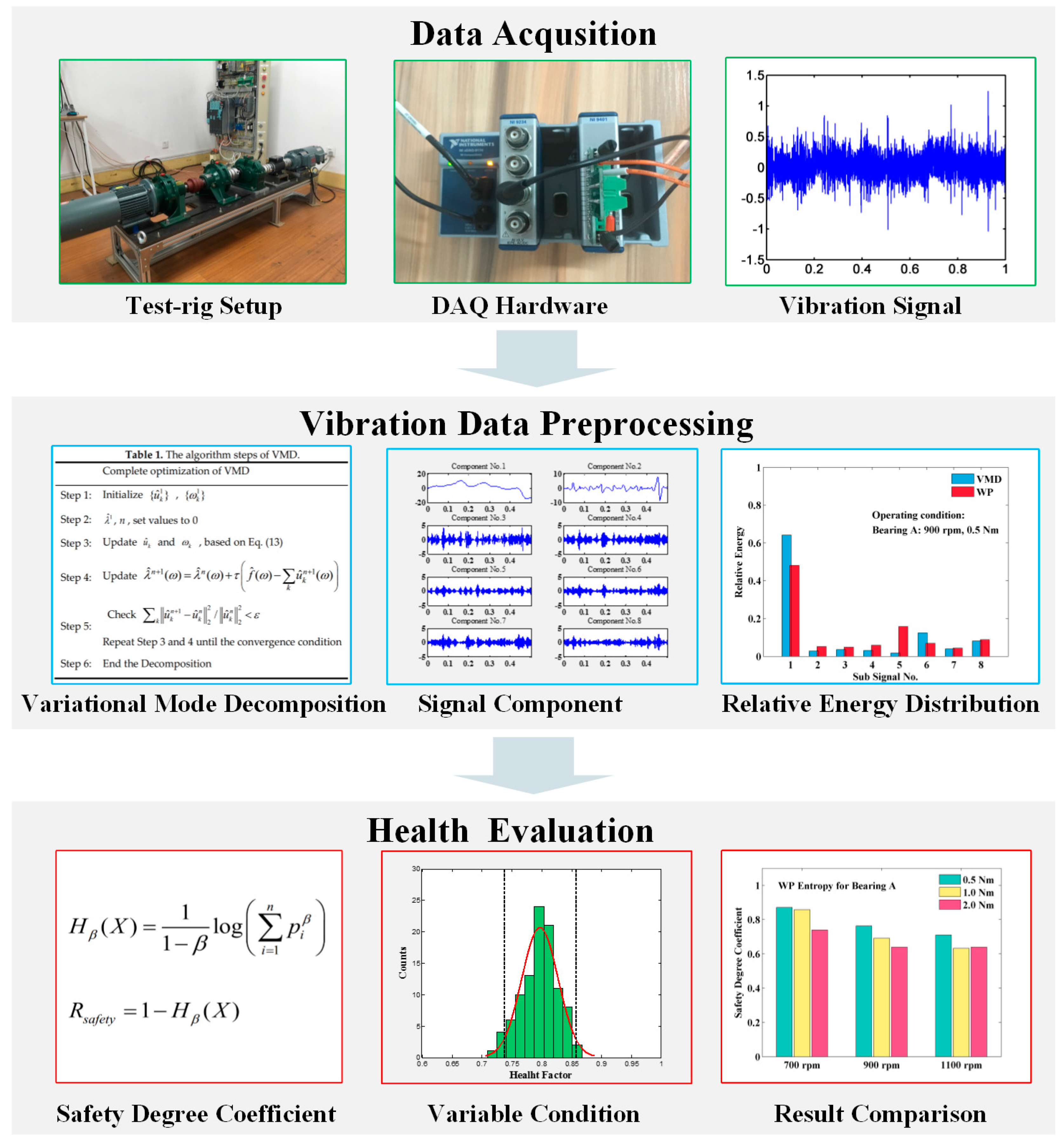
:Condition monitoring (CM) is used to assess the health status of wind turbines (WT) by detecting turbine failure and predicting maintenance needs. However, fluctuating operating conditions cause variations in monitored features, therefore increasing the difficulty of CM, for example, the frequency-domain analysis may lead to an inaccurate or even incorrect prediction when evaluating the health of the WT components. In light of this challenge, this paper proposed a method for the health evaluation of WT components based on vibration signals. The proposed approach aimed to reduce the evaluation error caused by the impact of the variable operating condition. First, the vibration signal was decomposed into a set of sub-signals using variational mode decomposition (VMD). Next, the sub-signal energy and the probability distribution were obtained and normalized. Finally, the concept of entropy was introduced to evaluate the health condition of a monitored object to provide an effective guide for maintenance. In particular, the health evaluation for CM was based on a performance review over a range of operating conditions, rather than at a certain single operating condition. Experimental investigations were performed which verified the efficiency of the evaluation method, as well as a comparison with the previous method.
1. Introduction
In response to the global energy crisis and the desire to reduce fossil fuel usage, wind energy has become one of the most promising renewable energy sources due to its environmentally friendly, socially beneficial, and economically competitive characteristics. Condition monitoring (CM) is one of the best approaches to increase the availability and reduce the operations and maintenance costs for wind turbines (WTs). Condition monitoring systems [1,2] include sensors and signal processing equipment to provide continuous indications of the state of a component, and are based on techniques including vibrational analysis, acoustics, oil analysis, strain measurement, and thermography. Furthermore, monitoring may be on-line to obtain the condition status in real time, or off-line to analyze the collected data in detail [3]. With guidance from the condition monitoring, maintenance tasks can be arranged in a reasonable schedule to prevent serious damage or WT failure [4].
To date, considerable effort has been expended in the development of CM and other technological innovations [5,6,7,8]. Vibration analysis remains the most popular technology in wind turbines, particularly for rotating equipment [9,10,11]. Many studies have been developed to enhance vibrational signal processing in CMs such as short-time Fourier transform (STFT) and the Wigner-Ville distribution (WVD) [12,13,14]. Alternatively, wavelet transform [15,16] is a time-frequency technique similar to short-time Fourier transform (STFT), but is more appropriate for non-stationary signals with variable time-frequency resolution [17]. The wavelet transform presents a time-frequency three-dimension graph that decomposes the signal into a series of sub-signals or levels with different frequencies. The wavelet transform is effective and reliable compared to other vibration analyses [18,19]. Nonetheless, considering the linear expansion in a single basis, neither the Fourier transform nor the wavelet transform is sufficiently flexible. As a result, the wavelet packet transform (WPT) [20] was developed using a rich library of redundant bases with arbitrary time-frequency resolution. The wavelet packet coefficient set represents a signal with good local properties in the time-frequency resolution and extracts the transient characteristics, which is more efficient than STFT. In addition, S-transform is superior in the condition monitoring of wind turbines as it eliminates the limitations of STFT and wavelet transform. Furthermore, it also has more advantages in the time-frequency analysis of non-stationary signals [21]. However, a challenge still exists due to the poor local adaptive resolution. Hence, the empirical mode decomposition (EMD) is attractive in signal processing for its local adaptive feature [22]. The EMD is widely applied in CM WTs for its superior abilities to process nonlinear and non-stationary signals [23,24]. Nevertheless, the EMD decomposes the CM signal in recursive calculation, which limits its application due to several drawbacks: (1) The efficiency of the EMD is decreased in the processing period since the algorithm of the EMD adopts recursive calculation; (2) The error developed in the upper and lower envelop estimation will spread in the recursive decomposition results; and (3) The intrinsic mode functions decomposed by the EMD are not band-limited, which creates a mode mixing problem. As a consequence, there have been many studies using EMD, such as the application of ensemble EMD and bivariate EMD in the condition monitoring of wind turbines [25,26].
To overcome the shortcomings of the EMD, variational mode decomposition (VMD) has been recently proposed as an alternative for EMD to separate the composite real-valued time series into their respective modes [27]. In contrast to the EMD, the VMD decomposes a signal into several principal modes, which are updated with the Wiener filter, and the central frequency of each mode is gradually demodulated to the corresponding baseband. It is noted that VMD is theoretically much better than sequential iterative sifting of the EMD as VMD is based on a clear variational model and the resulting minimization steps extract the concurrent mode intuitively. As attributed by the Wiener filter, the mode bandwidth decomposed by VMD is narrow, which not only overcomes the mode mixing problem in the EMD, but also guarantees the accurate extraction of the time-frequency features. Furthermore, by adopting non-recursive calculations, the VMD is more efficient than the EMD in computing performance. In addition, the VMD is more robust when addressing noise and has stronger local decomposition abilities than EMD-based methods. Moreover, the instantaneous frequency spectra generated by VMD has a higher resolution in both time and frequency than that of STFT and WPT [28].
With the highlighted competitive advantage of the VMD, many researchers have tried to enhance its potential application in CM signal feature extraction. Wang et al. [29] investigated the equivalent filtering and the applications on rotor-stator fault diagnosis, and proved its validity in detecting rubbing-caused multiple features. Li et al. [30] proposed an independence-oriented VMD method to adaptively extract the weak and compound fault features of the wheel set bearing via correlation analysis where the appropriate mode number was determined by the criterion of approximate complete reconstruction. In [31], a performance comparison of the VMD and the empirical wavelet transform (EWT) was discussed regarding the classifying ability of the power quality by using supported vector machine. Their results showed that the VMD performed better than the EWT in feature extraction. To alleviate the negative influence of wind power generation, Zhang et al. [32] proposed a VMD-based novel model to improve the predicating performance of the short-term wind power.
As mentioned above, these vibration-based approaches for the condition monitoring of rotational machines have been mostly developed for certain fixed operating conditions. When considering the non-linear control behavior of wind turbines [33,34,35], the acquisition data varies over a wide range of operating conditions [36], therefore, both the rotation speed and torque load also varies over the fluctuated ranges [37]. The changing feature obtained from the measured data does not necessarily represent a problem with the turbine. Conversely, variations in an extracted feature only indicate a change in the operating conditions, which significantly increases the difficulty of condition monitoring. Therefore, an adaptive data pre-processing technique is indispensable for extracting valid features from the monitored components while normalizing the operational and environmental parameters. For instance, Igba et al. [38] proposed a novel condition monitoring method based on the signal correlation, extreme value, and root-mean-square (RMS) of the vibration signal to indicate early fault detection. The results showed that the correlation between the signal and RMS values were sensitive to failure detection in high speed bearing pitting and shaft cracks. Baydar and Ball [39] performed gear deterioration detection under different loads by using the instantaneous power spectrum and the WVD. Furthermore, they successfully performed gear fault detection, and indicated that the gear faults were irrespective with variable operating conditions. Similarly, Fan and Zuo [40] combined Hilbert and wavelet packet transforms to detect gear faults with the ability for handling non-stationary signals. As WT components are often operated at variable wind speed, the CM signals of WTs always contain intra-wave features, which increases the difficulty in fault extraction. Yang et al. [41] adopted the VMD method to monitor the conditions when extracting features of wind turbines. The experiment verified that the VMD performed better than the EMD, not only in noise robustness, but also in multi-component signal decomposition, side-band detection, and intra-wave feature extraction.
From an information entropy theory perspective, the most uncertain probability distribution has the largest entropy, and the entropy of the most certain probability distribution has the smallest entropy. Based on this background, the information entropy theory is widely used in machinery condition monitoring and fault diagnosis. Sawalhi et al. [42] developed a fault detection method for the roller bearings based on the minimum entropy and spectral kurtosis. Tafreshi et al. [43] utilized entropy measurement and energy map to realize the fault feature extraction and the classification of machinery fault diagnosis. He et al. [44] used the approximate entropy as a nonlinear feature parameter to measure the irregularity of the vibration signals for fault diagnosis in rotating machinery. Their experimental results indicated that the approximate entropy was effective in distinguishing four typical faults including imbalance, misalignment, shaft rubbing, and oil whirl in rotation machines. In [45], a novel approach based on Renyi entropy derived from coefficients of the wavelet packet transform was developed for the diagnosis of gearboxes in presumably non-stationary and unknown operating conditions. The fault detection capabilities were verified efficiently by various seeded mechanical faults of the two-stage gearbox operation under different rotational speeds and loads.
In this paper, an alternative approach to health evaluation was proposed that was adapted to the varying operating condition. In particular, the vibration signal from the monitored object was decomposed into a set of sub-signals using VMD. Then, the energy of each sub-signal and the probability distribution of the energy at each sub-signal band was analyzed. Finally, the concept of entropy was introduced to evaluate the health condition of the monitored object. The novelty of the proposed approach included the following: (1) the health evaluation of CM was based on a review of the experimental performance over a range of operating conditions rather than on a certain operating condition; (2) the proposed approach reduced evaluation errors caused by the varying operating conditions; and (3) experimental investigations were performed to verify the efficiency of the evaluation method by comparing it with a previously used method.
The remainder of this paper is organized as follows. Section 2 presents a review of condition monitoring theory. Section 3 describes the experimental setup and the proposed method for operational safety evaluation based on the variational mode decomposition Renyi entropy. Section 4 contains the experimental description, together with several experimental studies and discussion. In Section 5, we provide our conclusions.
2. Review of Condition Monitoring Theory
2.1. Rolling Bearing Kinematics
Roller bearings are a key component of wind turbines. Before analyzing the bearing kinematics, some assumptions are made about the bearing systems: (1) that the outer and inner races move at a constant angular velocity; (2) all the elements in the bearing contact rigidly; (3) all the elements move without any slip; and (4) the contact angle is constant during the operation. For constant speed operations, the expression for the rolling element pass frequencies in the inner race (BPFI), the rolling element pass frequencies in the outer race (BPFO), and the rolling element spin frequency (BSF), which are important indicators to identify bearing faults, given as follows [46]:
where Nb is the number of rolling elements; fo is the rotation frequency of the outer race; fi is the rotation frequency of the inner race; d is the diameter of the rolling element; D is the pitch diameter of the bearing; and φ is the contact angle. Since the outer race is installed to be stationary in most cases, the rotation frequency of the outer race fo is equal to 0.
2.2. Wavelet Packet Decomposition
The wavelet packet transform (WPT) [45] was constructed and is schematically presented via a wavelet packet tree in Figure 1.
Each node of the WPT tree is marked by order (d, n), where d represents the current depth of the WPT tree, and n stands for the node number at the corresponding depth d. The node order n shows the relationship with the depth d as n = 0, …, 2d − 1. Each node in the decomposing level n, contains a wavelet packet coefficient Pjn(k), k = 0, …, Nd − 1, which is expressed as follows:
Each node of the wavelet packet tree can be approximately used as a band-pass filter at the specific frequency range. By calculating the power for each node, the probability distribution of the energy is determined and analyzed at each frequency band. The energy of the decomposed signal at node (d, n) is shown in Equation (5):
The total signal’s energy can be calculated by summing the energy at each terminal node. Then, the energy probability distribution can be estimated over the frequency range:
2.3. Variational Mode Decomposition
As an alternative method, the variational mode decomposition (VMD) [27] decomposes a signal into a discrete number of quasi-orthogonal band-limited sub-signals. These sub-signals possess certain sparse properties of the bandwidth in the spectrum domain, which determines the relevant bands adaptively and estimates the corresponding modes concurrently. The details of the VMD are as follows. To determine the bandwidth of each mode, the VMD first converts the mode uk into an analytic signal uk+ using the Hilbert transform with a single sided frequency spectrum as shown in Equation (8):
Then, the mode’s frequency spectrum is shifted to the baseband, adjusting the corresponding estimated center frequency using the exponential term. Utilizing the squared L2-norm of the gradient, the bandwidth is estimated from the Gaussian smoothness. The VMD method can be written as a constrained variational problem:
where {uk}: = {u1, …, uK} and {ωk}: = {ω1,…, ωK} represent the set of all modes and the relevant center frequencies. The reconstruction constraint in Equation (10) can be addressed via a quadratic penalty term and Lagrangian multipliers as follows:
The Alternate Direction Method of Multipliers (ADMM) is utilized to determine the saddle point of the augmented Lagrangian in a sequence of iterative sub-optimizations, the details of which are provided in References [39,40,41]. In this approach, all modes are obtained and updated using Wiener filtering to tune the relevant center frequency on the spectrum:
The center frequency is obtained at the weighted center of the power spectrum for each mode. This mean carrier frequency is the frequency for a least squares linear regression of the instantaneous phase observed in the mode. The VMD algorithm is shown in Table 1.
2.4. Renyi Entropy
As a method to quantify the diversity, uncertainty, and randomness of the system in information theory, the Renyi entropy is introduced as the indices of diversity in statistics, which is defined as:
where β ≥ 0 and β ≠ 1; and X is a discrete random variable with possible outcomes; and the corresponding probabilities are pi. The parameter α has a significant effect on the statistical result of the Renyi entropy in Reference [47]. As β increases, the sensitivity to a small probability event will decrease as the statistical range of the Renyi entropy expands simultaneously. In contrast, as β decreases, the sensitivity to a small probability event increases and the statistical range shrinks. Therefore, the value of β needs to be adjusted appropriately based on the signal features of the transient components since the components of the signal are influenced by the low energy.
3. Proposed Method
3.1. Experimental Setup
To examine the performance of the proposed approach under fluctuating operating conditions, a motor-drive test-rig was built as seen in Figure 2. Due to the large size of the real turbine and difficulty with the test, the test-rig was designed in a scaled-down size for the laboratory environment. The test-rig consisted of two three-phase asynchronous induction motors on a fixed test-bed, where one acted as a prime mover in torque mode, and the other as an electric generator in speed mode. The induction motors were controlled by a high-performance driver (Siemens SINAMICS S120 system (2008, Siemens, Munich, Germany)). Both torque and speed curves were obtained under computer supervision using the Profinet protocol. Considering that the transmission of the variable-speed wind turbine consisted of a two-stage planetary gearbox with one-stage parallel, the experimental setup selects a parallel shaft gearbox to simulate the parallel axes stage of the wind turbine gearbox. In this test-rig, the bearing fixed in the gearbox operated at different rotation speed and load conditions. Hence, the simulator setup acted as an integral system of the wind turbine. In this case, the roller bearing fixed in the gearbox was operated in a simulating condition like wind turbines. Additionally, a torque-tachometer r was installed between the generator and the gearbox to measure the torque and rotation speed of the bearing to monitor the real time operational conditions. Moreover, a National Instruments (NI) cDAQ-9174 chassis (2012, National Instruments, Austin, TX, USA), in combination with a digital Input/Output module NI-9401 and an analog voltage input module NI-9234, was used to provide a frequency counter and A/D converter for signal acquisition. An integral electronic piezoelectric (IEPE) accelerometer was connected to the NI-9234 module to determine the vibration signal from the tested bearing. The torque-tachometer output two digital signals to the NI-9401, where one represented the torque signal in an impulse sequence for a specific frequency, and the other the rotation pulse from the optical encoder in the tachometer. Details on the data acquisition system are shown in the Appendix A. The setup of the experimental test-rig is shown in Figure 3.
3.2. Health Evaluation Using VMD Renyi Entropy
As mentioned previously, there are many methods to analyze vibration monitoring signals, such as root mean square (RMS), kurtosis, zero order figure of merit (FM0), etc., for observations over a broad frequency range. The operational safety degree was increased in Reference [48] and the Renyi entropy defined as:
where is the probability distribution of the energy in the frequency domain; and β is the parameter defined in the Renyi entropy, which was set to 0.8 in the following experiment.
In this paper, we developed an approach to health evaluation based on VMD with the Renyi entropy for condition monitoring. The test-rig was built in a scaled-down size for the laboratory environment, which aimed at focusing on the roller bearing in the gearbox. Although the size of the bearing was scaled down, the structure of the roller bearing was same as the one in the parallel axes stage of a real wind turbine box. The vibration signal of the bearing in the time domain was acquired on the test-rig setup using the NI-9234 hardware. The rotation speed and transfer torque were obtained using the NI-9401 to monitor the experimental performance, rather than for the proposed condition monitoring. Then, the vibration signal was processed using the variational mode decomposition method to obtain the sub components for the proposed numbers, based on Section 2.3. By calculating the relative energy distribution of the sub signal components, we defined the variational mode decomposition entropy to evaluate the condition of the bearings at an uncertain operating state. A schematic diagram is presented as Figure 4, with a comparison to show the effectiveness of the proposed method in the ninth sub-picture.
4. Experiment and Discussion of Results
4.1. Experimental Description
To evaluate the effectiveness of the proposed method, an experimental study was performed on the test-rig to monitor the condition of the rolling bearings. The vibration signals from the tested bearings were detected by a piezoelectric acceleration sensor, located on the gearbox on top of the bearings. Details of the piezoelectric acceleration sensor are listed in the Appendix A. The sampling frequency was 2 kHz and the length of each sampling time was 1 s. Moreover, the rotation speed and torque were collected to track the operating condition in real time.
For the experiments, two tapered roller bearings were selected as the test bearings to simulate four different health statuses. These were marked as Bearing A or B. The details of the selected bearings are presented in the Appendix A. Defects in the outer races were introduced as small rectangular slits cut using electro-discharge machining. The rectangular slit in Bearing A was 1 mm wide and 1 mm deep. The rectangular slit in Bearing B was 2 mm wide and 2 mm deep, which corresponded to slight wear in A and serious wear in B.
These selected bearings were all operated under different speeds and loads to study their effect on the behavior of the bearing vibration. In particular, the drive speeds of the input axis were 700, 900, and 1100 rpm and the load torques were 0.5, 1, and 2 Nm, respectively. Moreover, the tested bearing was located at the output axis of the gearbox and the transmission ratio was 1:1.41. Thus, the output axis rotation speed was 987, 1269, and 1551 rpm. Substituting these parameters based on the kinematic parameters of the tested bearings and rotational speed, the corresponding fault frequency of the outer race as determined as 7.3fn, where fn is the shaft speed in Hertz. As a result, the characteristic bearing defect frequencies of the outer race were 120.1 Hz, 154.4 Hz, and 188.7 Hz, respectively. Table 2 provides a quick insight into the detail of the operating condition setting and the characteristic defect frequencies as follows.
4.2. Basic Analysis Characteristics
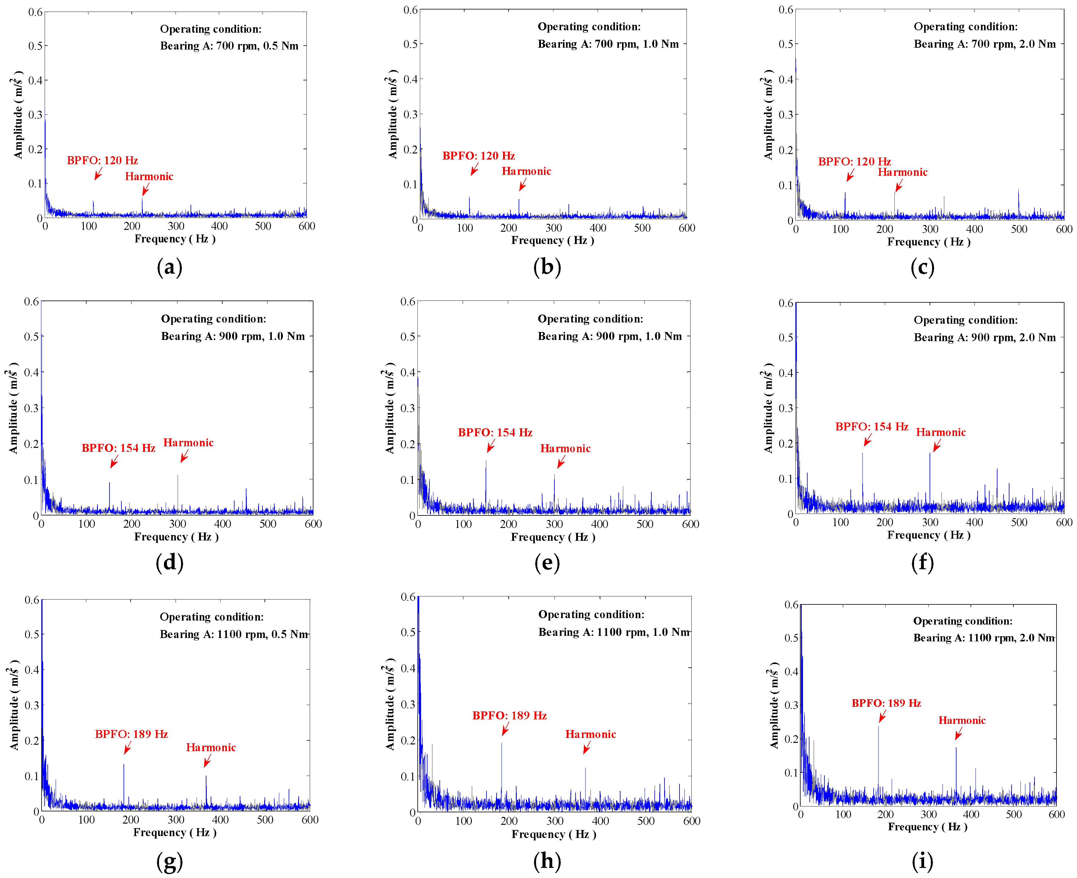
As above-mentioned, time and frequency domain analyses are basic and useful for condition monitoring. The vibration signal waveforms in the time domain combined with the amplitude spectrum for Bearing A in the frequency domain are shown in Figure 5. The peak values of the accelerations were apparent at the characteristic defect frequencies for the wearing bearings. This showed that fluctuating operating conditions affected the amplitude spectrum at the characteristic frequencies. For instance, the amplitudes at the characteristic defect frequencies increased by approximately 0.1 m/s2 as the load torque increased for the 1100 rpm condition in Figure 5g,i. Meanwhile, the amplitudes at the characteristic defect frequencies increased approximately 0.2 m/s2 as the rotation speed increased from 700 rpm to 1100 rpm for the 2 Nm loading condition in Figure 5c,i.
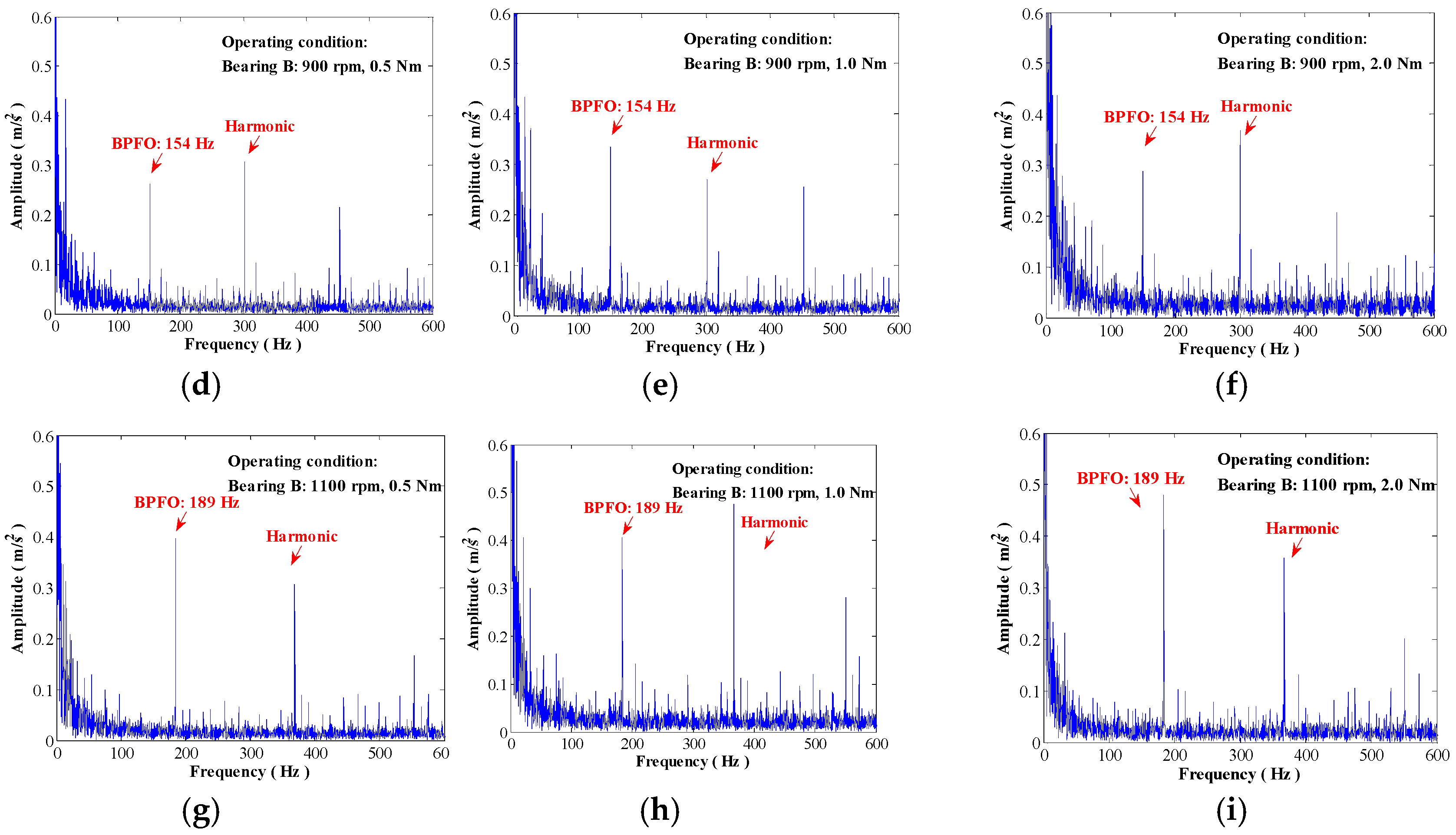
Figure 6 shows the amplitude spectrum for Bearing B for a clear comparison as follows. Based on this observation: (1) for a particular operating condition, Bearing B exhibited a higher amplitude than Bearing A; (2) for a particular bearing, the amplitude at the characteristic defect frequencies increased with the rotation speed of the shaft; (3) amplitude values at these characteristic points also exhibited slow growth as the shaft rotation torque increases; and (4) interestingly, under a high torque load and rotation speed (which is regarded as a serious operating condition), Bearing A exhibited a higher amplitude than Bearing B, which was operated under a low load and rotation speed. Although the wearing status in Bearing B was twice as large as that of Bearing A, the operating condition of the high rotation speed and the heavy torque raised a stronger vibration feature at the characteristic frequency.
It could be referred that the transmission train delivered the higher power energy during the high rotation speed and the heavy torque, which excited the component to act in response to a higher vibration level. In view of this situation, it can be concluded that the operating condition had a significant impact on the vibration signal, which is a vital factor that cannot be ignored during the condition monitoring.
Therefore, the frequency-domain values of the signal not only depend on the health status of the bearings, but also rely on the operating conditions that describe the rotational torque and speed. As a consequence, frequency-domain analysis may lead to an inaccurate or even incorrect prediction for condition monitoring under fluctuating conditions, particularly when evaluating the health condition.
4.3. Decomposition and Health Evaluation
In light of the weakness of the frequency-domain analysis for different operating conditions, the probability distribution of the vibration signal was introduced to evaluate the health condition of the monitored bearing. Based on information theory, the mechanical faults of the bearing and the uncertain operating conditions can both affect the uncertainty of the vibration signal, leading to results with a lower degree of uncertainty. With the above analysis, the proposed health evaluation using VMD Renyi entropy (referred to in Section 3.2) was adopted to analyze the vibrational signal as an alternative approach. Figure 7 shows the decomposed sub signal obtained by the VMD for Bearings A and B. For the VMD processing approach, the decomposition result depends on the parameters α and K. It should be noted that first, when K was too small, the vibration signal was under-binned, thus, the decomposition modes was either shared by the neighboring when α was small, or mostly discarded when α as large. Second, when K was too large, the vibration signal was over-binned. Thus, the extra modes consisted of large noise when α was small, or the key components were shared by two or more modes when α was big. In other words, too few modes by decreasing K led to under-segmentation of the signal, while too many modes led to the duplication of the mode or extra noise in the mode. Fortunately, all these unexpected cases can be identified during the pre-processing stage. Therefore, the optimal process can be reached from a large amount of trial data in the pre-analysis. In this experiment, the optimal parameters were selected as α = 1200 and K = 8. The convergence criterion tolerance was selected as 0.01.
As observed, after the decomposition, the shock components appeared on the higher order sub-component in the time domain. Furthermore, we noted that the magnitude of the higher order sub-components increased with increasing rotation speeds and load torques, proving that the fluctuating condition did influence the time-domain behavior for condition monitoring. Moreover, when comparing Bearings A and B using the same operating condition, the shock components presented more obvious characteristics in terms of the bearing with the greatest degree of wear.
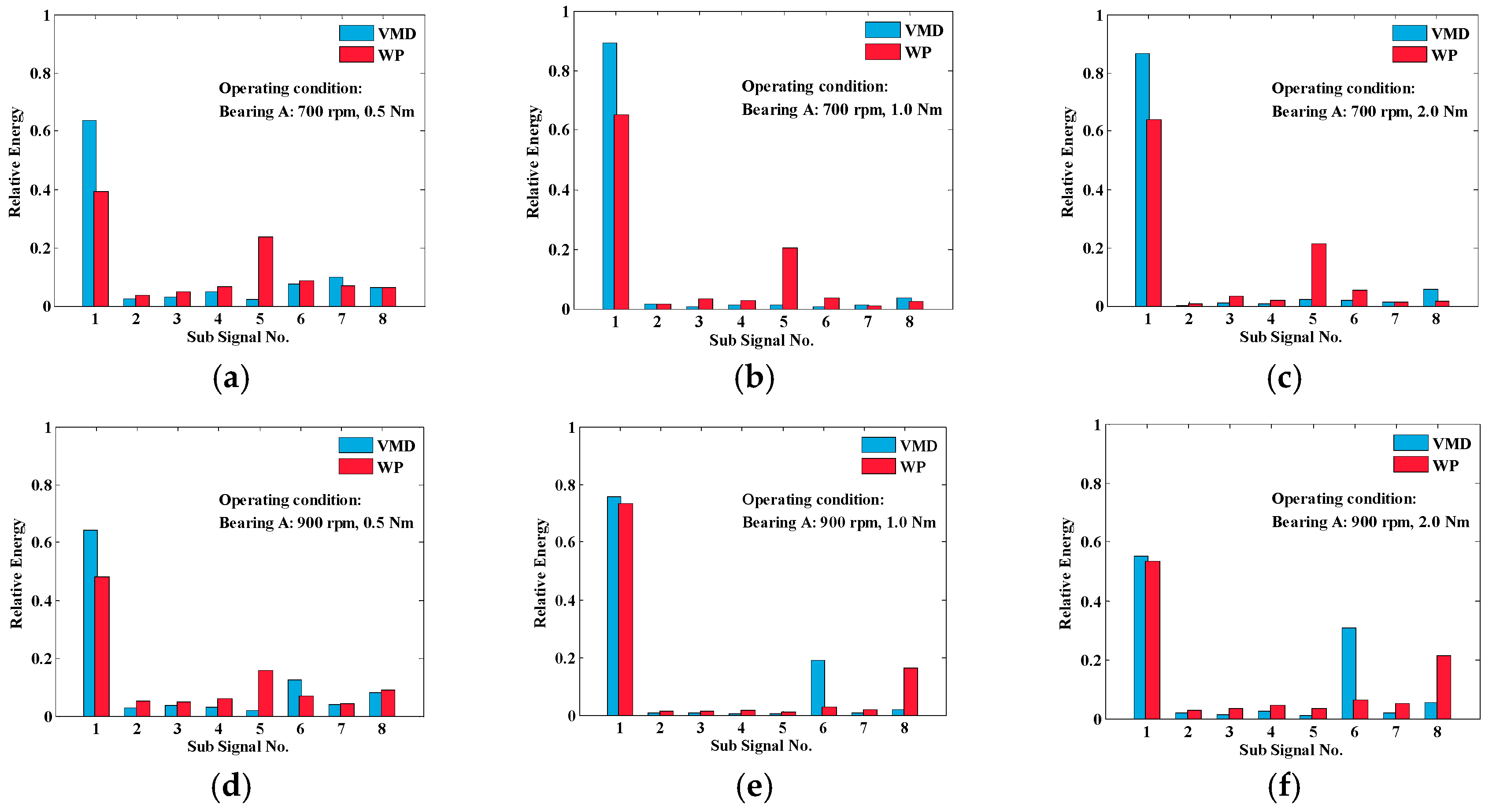
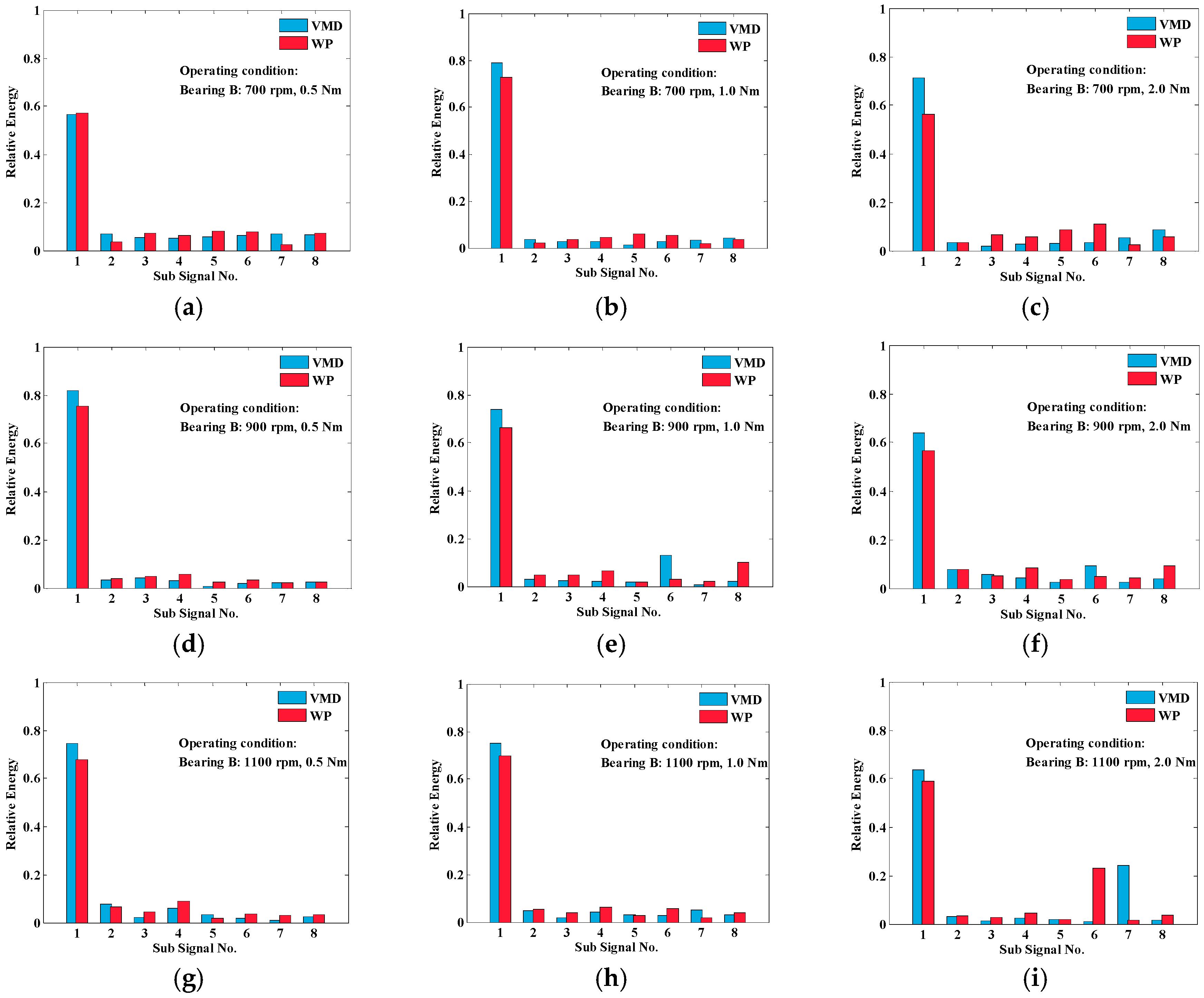
Next, the relative energy distribution was calculated as per Equation (12) based on the decomposed signal shown in Figure 8. Alternatively, wavelet packet decomposition was introduced to evaluate a healthy bearing as a comparison. The vibration signal of the bearings was also decomposed by Dmeyer (dmey) wavelet packet (WP) decomposition, with a level set to three. The terminal mode number for the wavelet packet was eight, as for the VMD numbers. By calculating the power for each node, the relative energy of the decomposed signal at all the terminal nodes was obtained using Equation (8). The relative energy distribution could also be performed using the VMD method.
As mentioned in Section 2, both the VMD and WP can be treated as a band-pass filter. Therefore, the relative energy distribution for each order component can describe the signal within a certain frequency band. As seen in Figure 9, the relative energy distributions for Bearing A calculated from the VMD and WP exhibited different trends.
This difference was mainly attributed to the lowest-frequency component, which is usually caused by the fluctuating operating conditions. In other words, VMD was better at mitigating the impact of the fluctuating conditions.
Additionally, Figure 10 presents the relative energy distribution calculated from the VMD and WP. A comparison with Figure 9 for Bearing A shows that the difference of the relative energy distribution of Bearing B under different operating conditions was relatively small. Therefore, it can be concluded that the increase of the bearing wear degree enhanced the fault characteristics, which led to the decrease of the analysis result.
Moreover, to decrease the random error in these experiments, a vibrational signal-acquisition experiment for each bearing was performed 50 times under different operating conditions, as shown in Table 2. The random condition for the rotation speed and the load torque was independent. For rotation speed, a set of random numbers ranging from 700 to 1100 was generated by the “rand” function on MATLAB. The count of the random number was 50. The generated random numbers were distributed continuously from 700 to 1100. However, the setting operating condition of the rotation speed in the experiments was 700 rpm, 900 rpm, and 1100 rpm, which was located as a separate step. Next, the generated random number was rounded approximately to the nearest discrete step in 700, 900, 1100. The random condition for the load torque as also generated, with the only difference being the random numbers ranging from 0.5 to 2. Finally, the random series of the rotation speed and the load torque were matched in one to one correspondence to generate the random operating condition. Figure 11 shows a histogram of the operational health degree coefficient for both the VMD Renyi entropy and WP Renyi entropy. The operational health degree coefficient exhibited an approximately normal distribution, and the 95% confidence interval is also marked. Since the random condition for the rotation speed was independent of the random condition for the load torque, the combination of the generated operating condition was random, also showing a normal distribution. As a result, the normally distributed result presented in Figure 11 indicated that the achieved result was reliable.
As presented in Figure 11 from the VMD Renyi entropy analysis, the average operational health degree coefficients for Bearings A and B were 0.778 and 0.401, respectively. In addition, the 95% confidence intervals of these health degree coefficients were 0.778 ± 0.055 and 0.401 ± 0.087. Meanwhile, the wavelet Renyi entropy concluded that on average, the operational health degree coefficient of Bearings A and B was 0.759 and 0.434, respectively. The 95% confidence intervals were 0.759 ± 0.122 and 0.434 ± 0.138, respectively. Thus, both analysis methods could represent the health status of the bearing. Bearing A (slight wear) indicated a high safety degree coefficient, whereas Bearing B (medium wear) indicated a lower coefficient. Additionally, we noted that the 95% confidence interval range for VMD entropy was approximately 50% less than for WP entropy.
Figure 12 shows a comparison between the VMD and the wavelet Renyi entropy analysis. The operational health degree coefficient, obtained from the vibrational signals from Bearings A and B for different operational conditions, were compared using the error statistics method. The VMD Renyi entropy had a better resistance performance than the wavelet Renyi entropy analysis. For Bearing A—based on the VMD—the safety degree coefficient decreased approximately 0.05, whereas the value decreased by approximately 0.06 for Bearing B. However, when adopting the WP method, the safety degree coefficient decreased more than 0.2 for Bearing B, which appeared as though the bearing was being continuously damaged under the fluctuating operational conditions. Thus, when the system was operated, the proposed VMD Renyi entropy analysis predicted a monitored bearing state more in-line with the real state, even if the monitored bearing was running at a faster rotation speed or heavier load. The difference in the confidence interval was the intrinsic distinction between the VMD and wavelet packet decomposition. The wavelet packet decomposition was approximately treated as a series of band-pass filters at the specific frequency range, where the bandwidth of each band-pass filter was fixed. Therefore, the probability distribution of the energy in the wavelet packet decomposition was located at each equal bandwidth frequency band. Additionally, as the wavelet packet decomposition relies on the selection of the wavelet base in practice, this would lead to the variation in the analysis result. In contrast, the variational mode decomposition decomposed the signals into a series of modes, where each mode was treated as an AM-FM signal. Each mode had a limited and narrow bandwidth, which shifted to baseband by mixing with a complex exponential of the current center frequency estimate. In this circumstance, the relevant center frequencies of each mode could be captured precisely, and the probability distribution of the energy was less affected under a different operating condition.
5. Discussion
According to Figure 5 and Figure 6, the bearing vibration varied over a wide range due to the influence of rotation speed and load torque. The reason for this is the variations in the transmission power at the macro stage, which led to the spectrum deviating from its normal position. For variable speed pitch-regulated WTs, their rotational speed and torque are precisely controlled to ensure efficient and safe power generation. As a consequence, nonlinearities caused by the pitch control should be considered in the rotation speed and torque.
Concerning the complex rotation speed and torque condition, VMD Renyi entropy analysis was carried out to provide a more reliable indication of the health status of WTs over a wide range of operating conditions. Furthermore, the wavelet Renyi entropy analysis was introduced as a comparison. As shown in Figure 11, both methods could identify the wear level of the bearings from the average values.
However, the average value of the operational health degree coefficient is based on large amounts of data acquisition at random operating conditions. Figure 11c,d shows an interval twice as wide as the one in Figure 11a,b. The operational health degree coefficient based on the wavelet packet Renyi entropy was much more affected by the variable operating conditions. In other words, the operational health degree coefficient based on the wavelet packet Renyi entropy exhibited significantly more variation as the operating conditions fluctuated. As a result, a potentially incorrect result may be generated for the condition monitoring system due to the variable speed or load. However, the VMD Renyi entropy had better clustering performance than the wavelet Renyi entropy analysis due to its compact interval for the fluctuating conditions.
The advantage of the relative energy distribution is that it depends on the variations of the vibration rather than the instantaneous values. Since VMD and WP decomposition may be roughly regarded as a series of band-pass filters, the relative energy distribution for each order component can describe the signal within a certain frequency band. Moreover, Figure 9 and Figure 10 showed that VMD was better at decreasing the impact of the fluctuating conditions in terms of the energy separation in the lowest-frequency component. As a consequence, VMD entropy provided the most reliable indication of the health status of a WT.
Although the proposed CM method of the VMD Renyi entropy presented a better result, there are still several points that need to be improved. As above-mentioned, the parameter K and α was vital to the decomposition result. The decomposition number K needed to be predefined, which is the same as other classical segmentation algorithms like wavelet packet transform. Both over-binning and under-binning had a negative impact on the detected mode. The value α also needs to be properly selected to capture the center frequency. Furthermore, the selection of the convergence criterion tolerance σ is vital to guarantee the success rate and the efficiency of the VMD algorithms. For instance, a low-noise level ensures an optimal result, but costs much more in calculation time. Additionally, given that wind turbines operate with variable speed, the spectrum bands of vibration signal would vary drastically over time. Nevertheless, the VMD does not work with non-stationary signals. An alternative choice is to break the signal composition down in a shorter time block. Hence, the vibration signal is approximately stationary in the short time.
Moreover, considering the control effects and influence of varying operational conditions, a reliable CM of WTs should be based on a review of WT general behavior over a range of operational conditions rather than its instantaneous responses. For instance, a large wind farm may consist of hundreds of WTs, costing millions of pounds to equip each WT. A false alarm caused by the operational conditions may result in long downtimes and high maintenance costs, leading to huge economic losses. In contrast, when vibration does not increase with the continued deterioration of a fault under low loads, the excessively long maintenance periods would lead to irreversible damage to the WT. Therefore, based on both cases, the proposed method to determine the health degree coefficient evaluation is essential and meaningful when properly planning maintenance schedules.
6. Conclusions
This paper presented a method for the health degree coefficient evaluation for a bearing under variable operational conditions. Using variational mode decomposition and optimized process parameters, the vibration signal was decomposed into a number of sub components. The calculation of the power for each component was used to analyze the probability distribution of the energy at each sub-component band. Subsequently, the Renyi entropy was introduced to evaluate the health of the bearings, namely, the operational safety coefficient for an uncertain operating state. Several experimental investigations were performed to validate the effectiveness of the proposed evaluation method for condition monitoring. The conclusions of this study are summarized as follows:
- (1)
- Frequency-domain amplitude of the vibrational signal is not only dependent on the health state of the bearings, but also relies on the operational conditions such as rotation torque and speed.
- (2)
- The evaluation of the probability distribution for the vibrational signal is more efficient than the time and frequency analyses, particularly for fluctuating operating conditions.
- (3)
- The improved evaluation algorithm based on the VMD Renyi entropy may decrease the impact of the fluctuating operating conditions and permit the identification of the real state of the bearing more effectively. The maximum error caused by the variable conditions was relatively small when compared to wavelet packet decomposition. Thus, the reliability of the CM result was significantly enhanced.
In future study, the parameters of the VMD will be optimized with the operating condition in real time using artificial intelligence in a more efficient way than is possible with the empirical method.
Acknowledgments
This work is supported by the National Science Foundation of China (Project Name: Research on fault recognition and diagnosis technology for wind turbines gearboxes based on product test data. No. 51275453).
Author Contributions
Each author contributed extensively to the preparation of this manuscript. Lei Fu and Xiaojun Zhou developed the setup of the experiment test-rig; Sheng Fang and Junqiang Lou performed the experiments; Lei Fu, Xiaojun Zhou, and Yanding Wei analyzed the data; and Lei Fu wrote the paper.
Conflicts of Interest
The authors declare no conflict of interest.
Appendix A

Table A1.
Parameters for the torque-tachometer.
| Specifications | Value |
|---|---|
| Torque range | ±20 Nm |
| Impulse frequency at zero point (torque) | 0 kHz |
| Impulse frequency at positive maximum scale point (torque) | 15 kHz |
| Impulse frequency at negative maximum scale point (torque) | 5 kHz |
| Rotation speed range | 5000 rpm |
| Encoder resolution | 1024 pulse/r |
Table A2.
Parameters for the piezoelectric accelerometer.
| Specifications | Value |
|---|---|
| Acceleration range | 50 g |
| Sensitivity | 96.7 mV/g |
| Frequency response range | 0.5 Hz–5 kHz |
| Constant current source supply | 2 mA |
Table A3.
Parameters for the tapered rolling bearing.
| Specifications | Value |
|---|---|
| Bearing type | 32,206 |
| Manufacturer | SKF, Goteborg, Sweden |
| Inner diameter | 30 mm |
| Outer diameter | 62 mm |
| Contact angle | 14° |
| Rolling element equivalent diameter | 8.5 mm |
References
- Pan, M.C.; Li, P.C.; Cheng, Y.R. Remote online machine condition monitoring system. Measurement 2008, 41, 912–921. [Google Scholar] [CrossRef]
- Hameed, Z.; Hong, Y.S.; Cho, Y.M.; Ahn, S.H.; Song, C.K. Condition monitoring and fault detection of wind turbines and related algorithms: A review. Renew. Sustain. Energy Rev. 2009, 13, 1–39. [Google Scholar] [CrossRef]
- Wei, J.; Liu, C.; Ren, T.; Liu, H.; Zhou, W. Online condition monitoring of a rail fastening system on high-speed railways based on wavelet packet analysis. Sensors 2017, 17, 318. [Google Scholar] [CrossRef] [PubMed]
- Scarf, P.A. A framework for condition monitoring and condition based maintenance. Qual. Technol. Quant. Manag. 2007, 4, 301–312. [Google Scholar] [CrossRef]
- Tchakoua, P.; Wamkeue, R.; Ouhrouche, M.; Slaoui-Hasnaoui, F.; Tameghe, T.A.; Ekemb, G. Wind turbine condition monitoring: State-of-the-art review, new trends, and future challenges. Energies 2014, 7, 2595–2630. [Google Scholar] [CrossRef]
- Liu, W.; Tang, B.; Jiang, Y. Status and problems of wind turbine structural health monitoring techniques in China. Renew. Energy 2010, 35, 1414–1418. [Google Scholar] [CrossRef]
- Cao, M.; Qiu, Y.; Feng, Y.; Wang, H.; Li, D. Study of wind turbine fault diagnosis based on unscented Kalman filter and SCADA Data. Energies 2016, 9, 847. [Google Scholar] [CrossRef]
- Muñoz, C.G.; Márquez, F.G. A new fault location approach for acoustic emission techniques in wind turbines. Energies 2016, 9, 40. [Google Scholar] [CrossRef]
- Feng, Z.; Ma, H.; Zuo, M.J. Vibration signal models for fault diagnosis of planet bearings. J. Sound Vib. 2016, 370, 372–393. [Google Scholar] [CrossRef]
- Roy, S.K.; Mohanty, A.R.; Kumar, C.S. Fault detection in a multistage gearbox by time synchronous averaging of the instantaneous angular speed. J. Vib. Control 2016, 22, 468–480. [Google Scholar] [CrossRef]
- Yen, G.G.; Lin, K.C. Wavelet packet feature extraction for vibration monitoring. IEEE Trans. Ind. Electron. 2000, 47, 650–667. [Google Scholar] [CrossRef]
- Uekita, M.; Takaya, Y. Tool condition monitoring technique for deep-hole drilling of large components based on chatter identification in time–frequency domain. Measurement 2017, 103, 199–207. [Google Scholar] [CrossRef]
- Tang, B.; Liu, W.; Song, T. Wind turbine fault diagnosis based on Morlet wavelet transformation and Wigner-Ville distribution. Renew. Energy 2010, 35, 2862–2866. [Google Scholar] [CrossRef]
- Hu, C.; Yang, Q.; Huang, M.; Yan, W. Sparse component analysis-based under-determined blind source separation for bearing fault feature extraction in wind turbine gearbox. IET Renew. Power Gener. 2017, 11, 330–337. [Google Scholar] [CrossRef]
- Rosso, O.A.; Martin, M.T.; Figliola, A.; Keller, K.; Plastino, A. EEG analysis using wavelet-based information tools. J. Neurosci. Methods 2006, 153, 163–182. [Google Scholar] [CrossRef] [PubMed]
- Liu, S.; Hu, Y.; Li, C.; Lu, H.; Zhang, H. Machinery condition prediction based on wavelet and support vector machine. J. Intell. Manuf. 2017, 28, 1045–1055. [Google Scholar] [CrossRef]
- Rehorn, A.G.; Sejdic, E.; Jiang, J. Fault diagnosis in machine tools using selective regional correlation. Mech. Syst. Signal Process. 2006, 20, 1221–1238. [Google Scholar] [CrossRef]
- Baydar, N.; Ball, A. Detection of gear failures via vibration and acoustic signals using wavelet transform. Mech. Syst. Signal Process. 2003, 17, 787–804. [Google Scholar] [CrossRef]
- Miao, Q.; Makis, V. Condition monitoring and classification of rotating machinery using wavelets and Hidden Markov models. Mech. Syst. Signal Process. 2007, 21, 840–855. [Google Scholar] [CrossRef]
- Ghaderi, H.; Kabiri, P. Automobile engine condition monitoring using sound emission. Turk. J. Electr. Eng. Comput. Sci. 2017, 25, 1807–1826. [Google Scholar] [CrossRef]
- Yang, W.; Little, C.; Court, R. S-Transform and its contribution to wind turbine condition monitoring. Renew. Energy 2014, 62, 137–146. [Google Scholar] [CrossRef]
- Li, H.; Zhang, Y.; Zheng, H. Hilbert-Huang transform and marginal spectrum for detection and diagnosis of localized defects in roller bearings. J. Mech. Sci. Technol. 2009, 23, 291–301. [Google Scholar] [CrossRef]
- Shen, Z.; Chen, X.; Zhang, X.; He, Z. A novel intelligent gear fault diagnosis model based on EMD and multi-class TSVM. Measurement 2012, 45, 30–40. [Google Scholar] [CrossRef]
- Li, Z.; Yan, X.; Tian, Z.; Quan, C.; Peng, Z.; Li, L. Blind vibration component separation and nonlinear feature extraction applied to the nonstationary vibration signals for the gearbox multi-fault diagnosis. Measurement 2013, 46, 259–271. [Google Scholar] [CrossRef]
- Wang, J.; Gao, R.X.; Yan, R. Integration of EEMD and ICA for wind turbine gearbox diagnosis. Wind Energy 2014, 17, 757–773. [Google Scholar] [CrossRef]
- Yang, W.; Court, R.; Tavner, P.; Crabtree, C. Bivariate empirical mode decomposition and its contribution to wind turbine condition monitoring. J. Sound Vib. 2011, 330, 3766–3782. [Google Scholar] [CrossRef]
- Dragomiretskiy, K.; Zosso, D. Variational mode decomposition. IEEE Trans. Signal Process. 2014, 62, 531–544. [Google Scholar] [CrossRef]
- Xue, Y.; Cao, J.; Wang, D.; Du, H.; Yao, Y. Application of the variational-mode decomposition for seismic time–frequency analysis. IEEE J. Sel. Top. Appl. Earth Obs. Remote Sens. 2016, 9, 3821–3831. [Google Scholar] [CrossRef]
- Wang, Y.; Markert, R.; Xiang, J.; Zheng, W. Research on variational mode decomposition and its application in detecting rub-impact fault of the rotor system. Mech. Syst. Signal Process. 2015, 60, 243–251. [Google Scholar] [CrossRef]
- Li, Z.; Chen, J.; Zi, Y.; Pan, J. Independence-oriented VMD to identify fault feature for wheel set bearing fault diagnosis of high speed locomotive. Mech. Syst. Signal Process. 2017, 85, 512–529. [Google Scholar] [CrossRef]
- Aneesh, C.; Kumar, S.; Hisham, P.M.; Soman, K.P. Performance comparison of variational mode decomposition over empirical wavelet transform for the classification of power quality disturbances using support vector machine. In Proceedings of the International Conference on Information and Communication Technologies (ICICT 2014), Kochi, India, 3–5 December 2014; Volume 46, pp. 372–380. [Google Scholar] [CrossRef]
- Zhang, Y.; Liu, K.; Qin, L.; An, X. Deterministic and probabilistic interval prediction for short-term wind power generation based on variational mode decomposition and machine learning methods. Energy Convers. Manag. 2016, 112, 208–219. [Google Scholar] [CrossRef]
- Merabet, A.; Keeble, R.; Rajasekaran, V.; Beguenane, R.; Ibrahim, H.; Thongam, J.S. Power management system for load banks supplied by pitch controlled wind turbine system. Appl. Sci. 2012, 4, 801–815. [Google Scholar] [CrossRef]
- Lai, W.; Lin, C.; Huang, C.; Lee, R. Dynamic analysis of Jacket Substructure for offshore wind turbine generators under extreme environmental conditions. Appl. Sci.-Basel 2016, 6, 307. [Google Scholar] [CrossRef]
- Hussein, M.M.; Senjyu, T.; Orabi, M.; Wahab, M.A.A.; Hamada, M.M. Control of a stand-alone variable speed wind energy supply system. Appl. Sci. 2013, 3, 71–76. [Google Scholar] [CrossRef]
- Simani, S. Overview of modelling and advanced control strategies for wind turbine systems. Energies 2015, 8, 13395–13418. [Google Scholar] [CrossRef]
- Santoso, S.; Le, H.T. Fundamental time–domain wind turbine models for wind power studies. Renew. Energy 2007, 32, 2436–2452. [Google Scholar] [CrossRef]
- Igba, J.; Alemzadeh, K.; Durugbo, C.; Eiriksson, E.T. Analysing RMS and peak values of vibration signals for condition monitoring of wind turbine gearboxes. Renew. Energy 2016, 91, 90–106. [Google Scholar] [CrossRef]
- Baydar, N.; Ball, A. A comparative study of acoustic and vibration signals in detection of gear failures using Wigner-Ville distribution. Mech. Syst. Signal Process. 2001, 15, 1091–1107. [Google Scholar] [CrossRef]
- Fan, X.; Zuo, M. Gearbox fault detection using Hilbert and wavelet packet transform. Mech. Syst. Signal Process. 2006, 20, 966–982. [Google Scholar] [CrossRef]
- Yang, W.; Peng, Z.; Wei, K.; Shi, P.; Tian, W. Superiorities of variational mode decomposition over empirical mode decomposition particularly in time–frequency feature extraction and wind turbine condition monitoring. IET Renew. Power Gener. 2017, 11, 443–452. [Google Scholar] [CrossRef]
- Sawalhi, N.; Randall, R.B.; Endo, H. The enhancement of fault detection and diagnosis in rolling element bearings using minimum entropy deconvolution combined with spectral kurtosis. Mech. Syst. Signal Process. 2007, 21, 2616–2633. [Google Scholar] [CrossRef]
- Tafreshi, R.; Sassani, F.; Ahmadi, H.; Dumont, G. An Approach for the Construction of Entropy Measure and Energy Map in Machine Fault Diagnosis. J. Vib. Acoust.-Trans. ASME 2009, 131, 024501. [Google Scholar] [CrossRef]
- He, Y.; Huang, J.; Zhang, B. Approximate entropy as a nonlinear feature parameter for fault diagnosis in rotating machinery. Meas. Sci. Technol. 2012, 23, 045603. [Google Scholar] [CrossRef]
- Bokoski, P.; Juricic, D. Fault detection of mechanical drives under variable operating conditions based on wavelet packet Rényi entropy signatures. Mech. Syst. Signal Process. 2012, 31, 369–381. [Google Scholar] [CrossRef]
- Randall, R.B.; Antoni, J. Rolling element bearing diagnostics—A tutorial. Mech. Syst. Signal Process. 2011, 25, 485–520. [Google Scholar] [CrossRef]
- Boskoski, P.; Gasperin, M.; Petelin, D.; Juricic, D. Bearing fault prognostics using Renyi entropy based features and Gaussian process models. Mech. Syst. Signal Process. 2015, 52, 327–337. [Google Scholar] [CrossRef]
- Zhang, X.; Wang, B.; Chen, X. Operational safety assessment of turbo generators with wavelet rényi entropy from sensor-dependent vibration signals. Sensors 2015, 15, 8898–8918. [Google Scholar] [CrossRef] [PubMed]
Figure 1.
Nodes of the wavelet packet tree.
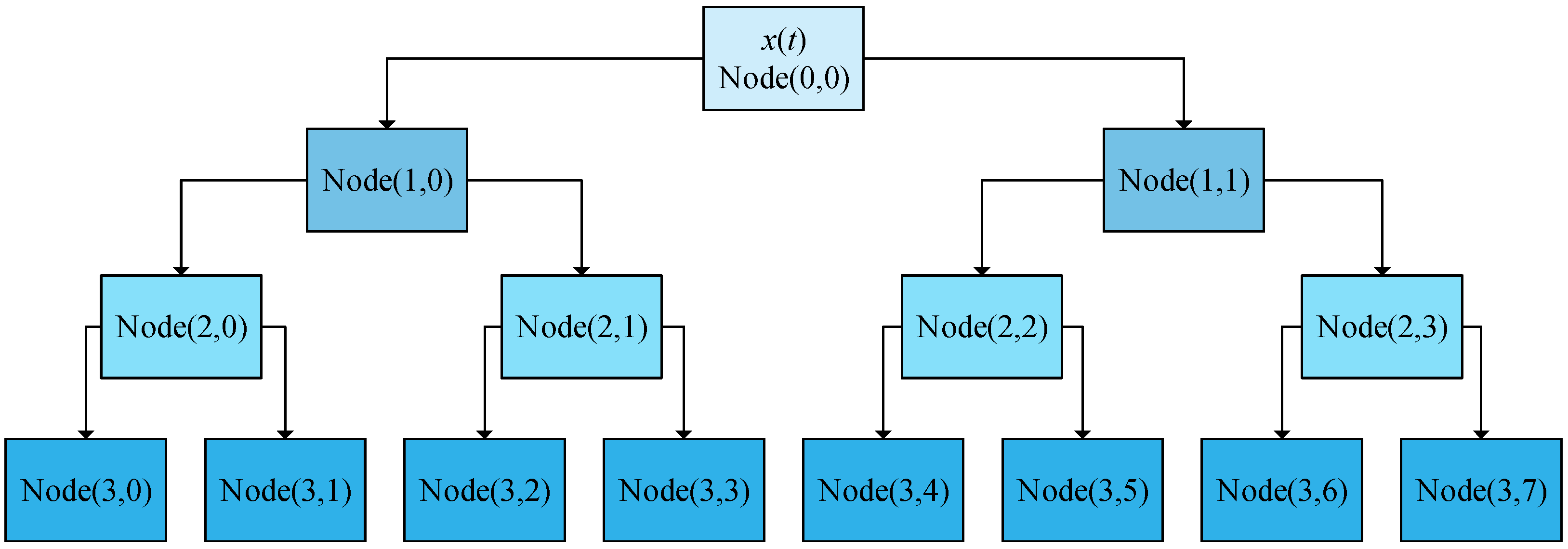
Figure 2.
Schematic diagram of the experimental test-rig.
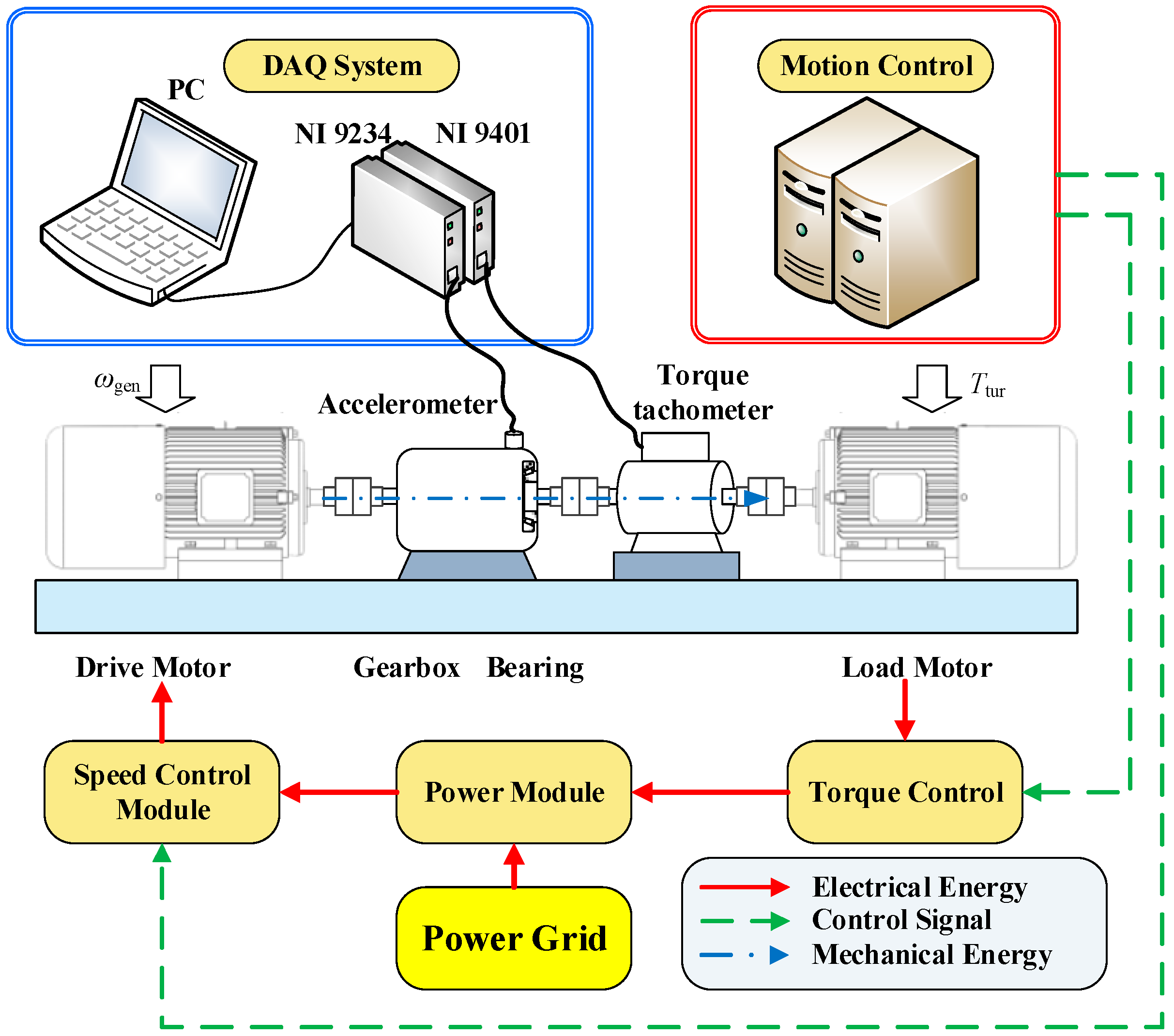
Figure 3.
Setup of the experimental test-rig.
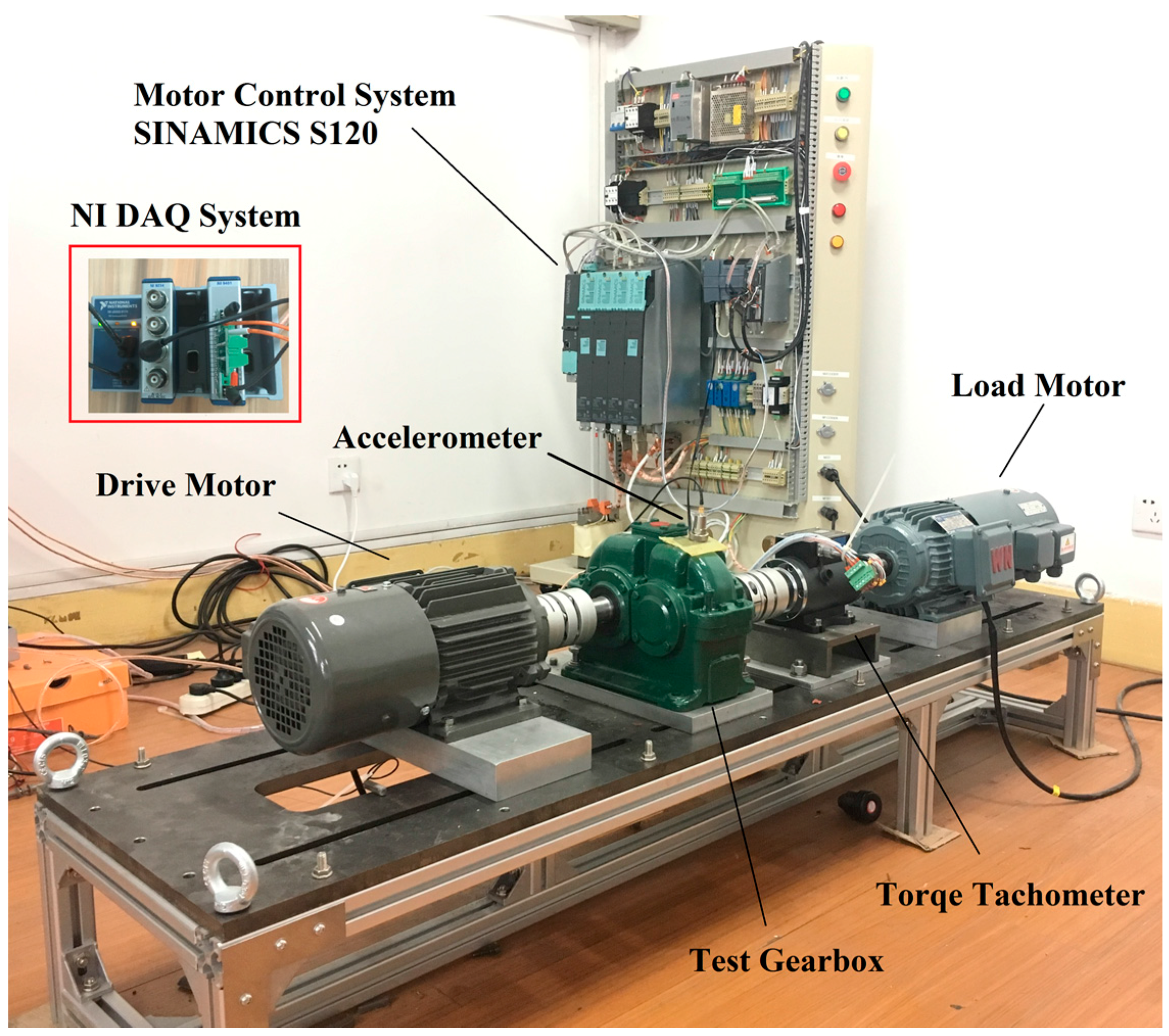
Figure 4.
Schematic diagram of the health evaluation using VMD entropy.

Figure 5.
Waveforms from Bearing A’s vibrational signal in the frequency domain. (a) Running in 700 rpm, 0.5 Nm; (b) Running in 700 rpm, 1.0 Nm; (c) Running in 700 rpm, 2.0 Nm; (d) Running in 900 rpm, 0.5 Nm; (e) Running in 900 rpm, 1.0 Nm; (f) Running in 900 rpm, 2.0 Nm; (g) Running in 1100 rpm, 0.5 Nm; (h) Running in 1100 rpm, 1.0 Nm; and (i) Running in 1100 rpm, 2.0 Nm.

Figure 6.
The waveform of Bearing B’s vibrational signal in the frequency domain. (a) Running in 700 rpm, 0.5 Nm; (b) Running in 700 rpm, 1.0 Nm; (c) Running in 700 rpm, 2.0 Nm; (d) Running in 900 rpm, 0.5 Nm; (e) Running in 900 rpm, 1.0 Nm; (f) Running in 900 rpm, 2.0 Nm; (g) Running in 1100 rpm, 0.5 Nm; (h) Running in 1100 rpm, 1.0 Nm; and (i) Running in 1100 rpm, 2.0 Nm.
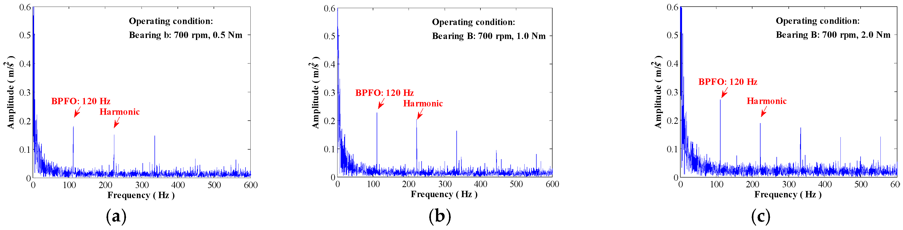

Figure 7.
The vibrational signal from Bearing A decomposed by VMD. (a) Running in 700 rpm, 0.5 Nm; (b) Running in 700 rpm, 1.0 Nm; (c) Running in 700 rpm, 2.0 Nm; (d) Running in 900 rpm, 0.5 Nm; (e) Running in 900 rpm, 1.0 Nm; (f) Running in 900 rpm, 2.0 Nm; (g) Running in 1100 rpm, 0.5 Nm; (h) Running in 1100 rpm, 1.0 Nm; and (i) Running in 1100 rpm, 2.0 Nm.
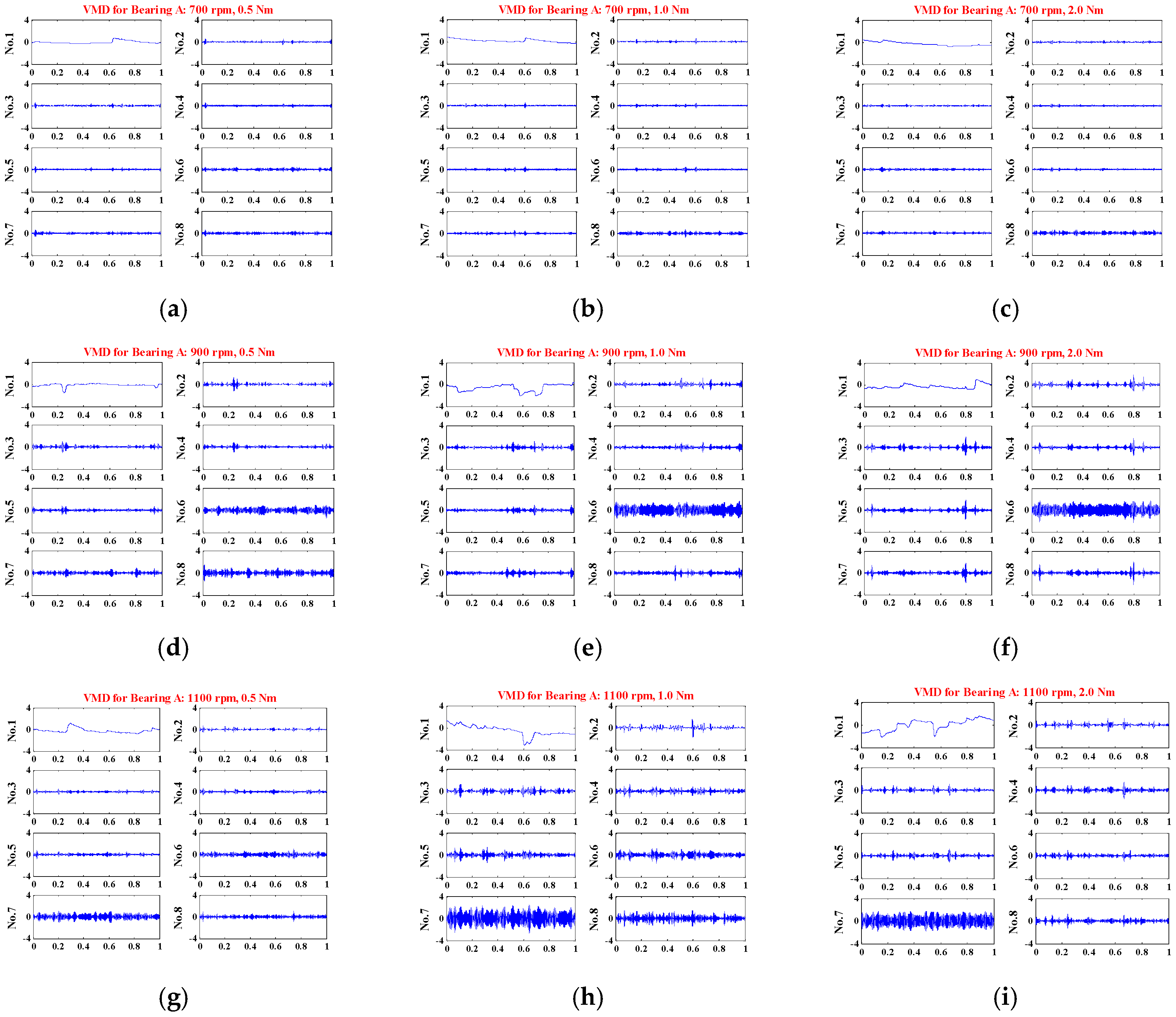
Figure 8.
The vibration signal from Bearing B decomposed by VMD. (a) Running in 700 rpm, 0.5 Nm; (b) Running in 700 rpm, 1.0 Nm; (c) Running in 700 rpm, 2.0 Nm; (d) Running in 900 rpm, 0.5 Nm; (e) Running in 900 rpm, 1.0 Nm; (f) Running in 900 rpm, 2.0 Nm; (g) Running in 1100 rpm, 0.5 Nm; (h) Running in 1100 rpm, 1.0 Nm; and (i) Running in 1100 rpm, 2.0 Nm.
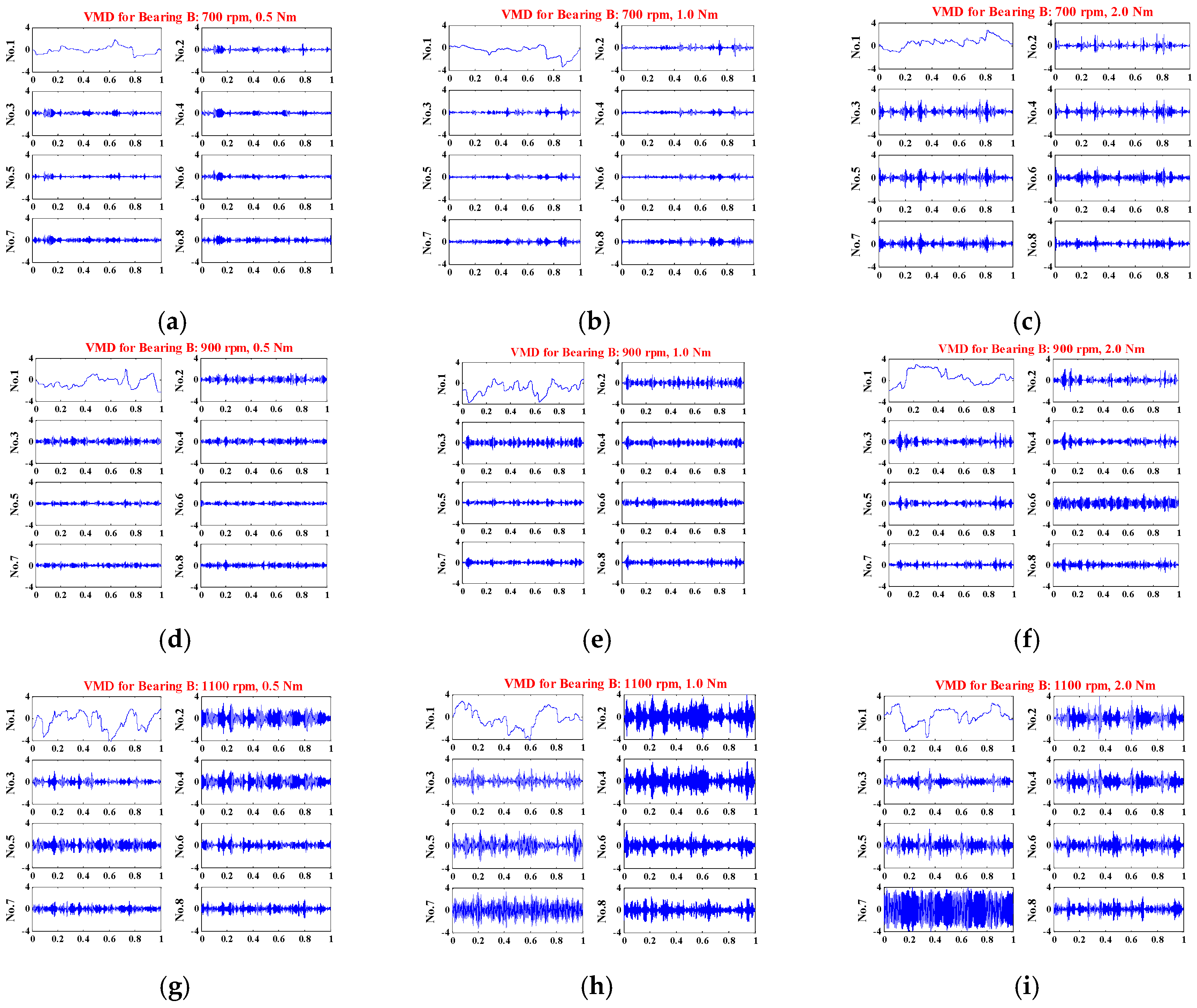
Figure 9.
The vibrational signal from Bearing B decomposed using wavelet packets. (a) Running in 700 rpm, 0.5 Nm; (b) Running in 700 rpm, 1.0 Nm; (c) Running in 700 rpm, 2.0 Nm; (d) Running in 900 rpm, 0.5 Nm; (e) Running in 900 rpm, 1.0 Nm; (f) Running in 900 rpm, 2.0 Nm; (g) Running in 1100 rpm, 0.5 Nm; (h) Running in 1100 rpm, 1.0 Nm; and (i) Running in 1100 rpm, 2.0 Nm.

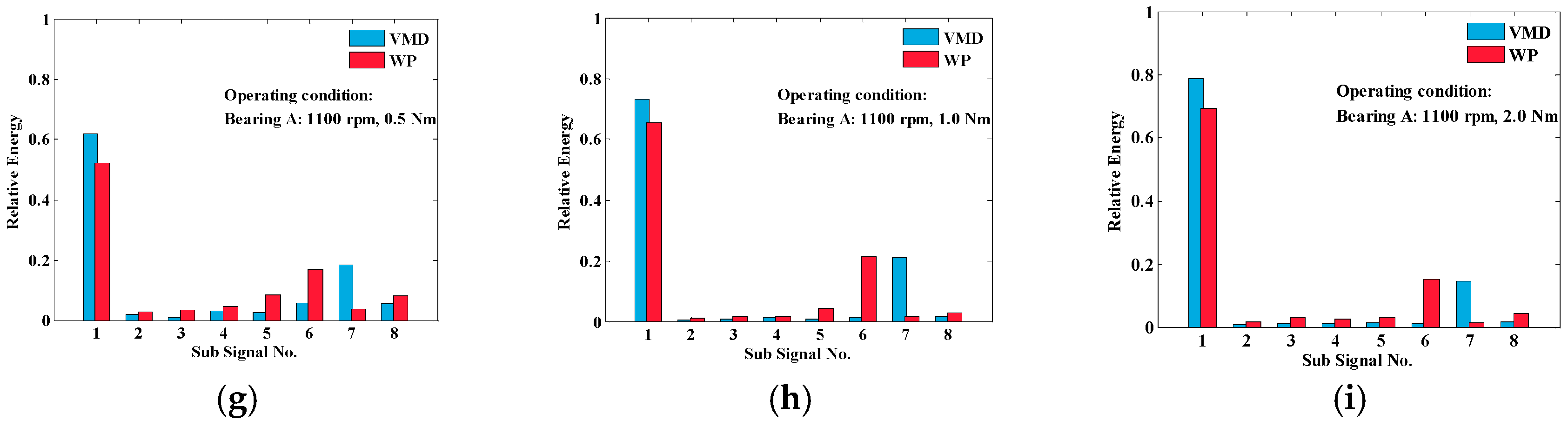
Figure 10.
The vibrational signal from Bearing B decomposed by WP. (a) Running in 700 rpm, 0.5 Nm; (b) Running in 700 rpm, 1.0 Nm; (c) Running in 700 rpm, 2.0 Nm; (d) Running in 900 rpm, 0.5 Nm; (e) Running in 900 rpm, 1.0 Nm; (f) Running in 900 rpm, 2.0 Nm; (g) Running in 1100 rpm, 0.5 Nm; (h) Running in 1100 rpm, 1.0 Nm; and (i) Running in 1100 rpm, 2.0 Nm.

Figure 11.
Histogram comparison of the safety degree coefficient. (a) The histogram of the safety degree based VMD entropy for Bearing A; (b) The histogram of the safety degree based VMD entropy for Bearing B; (c) The histogram of the safety degree based wavelet packets entropy for Bearing A; and (d) The histogram of the safety degree based wavelet packets entropy for Bearing B.
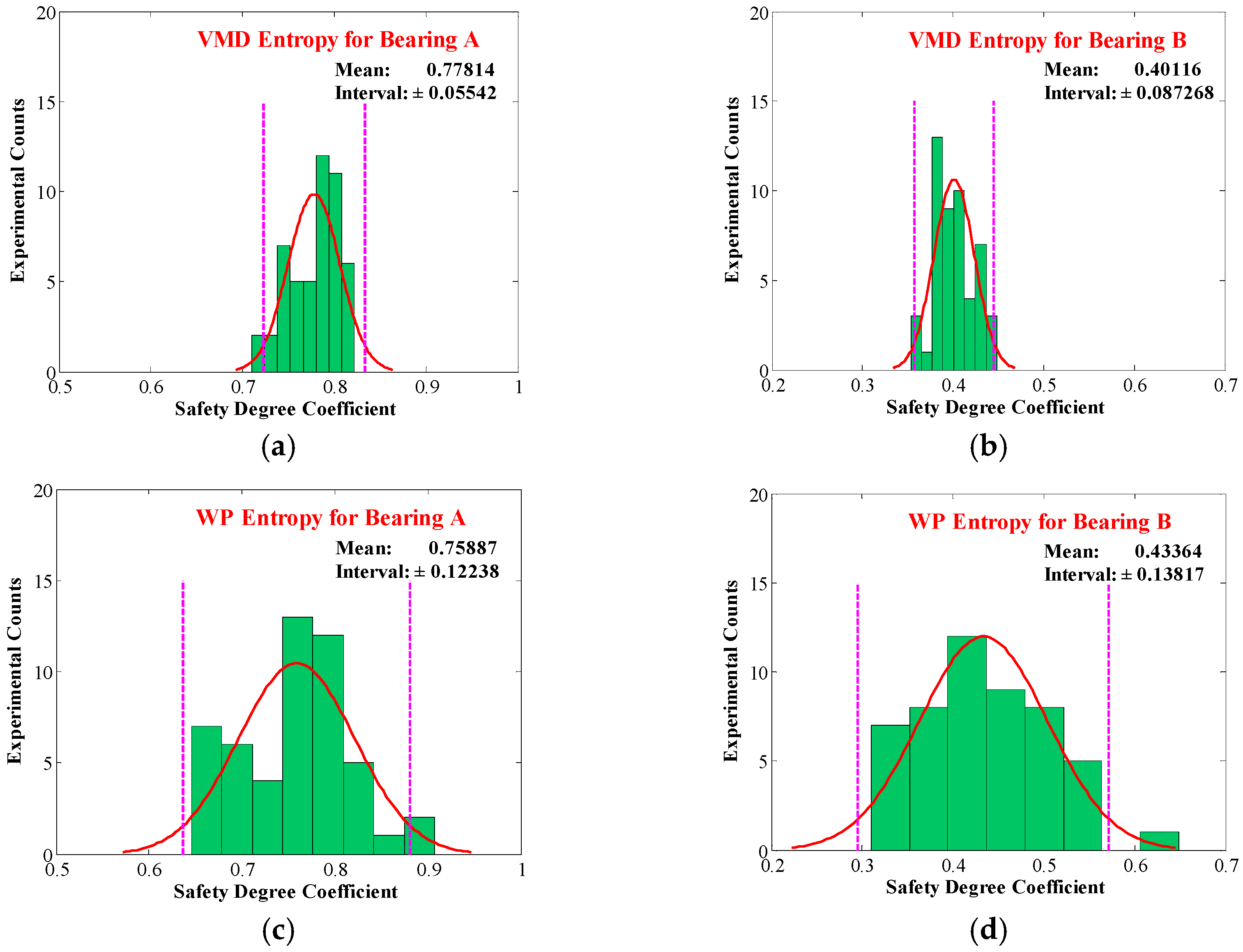
Figure 12.
Comparison of the safety degree coefficient for different conditions. (a) The safety degree based VMD entropy for Bearing A; (b) The safety degree based VMD entropy for Bearing B; (c) The safety degree based wavelet packets entropy for Bearing A; and (d) The safety degree based wavelet packets entropy for Bearing B.
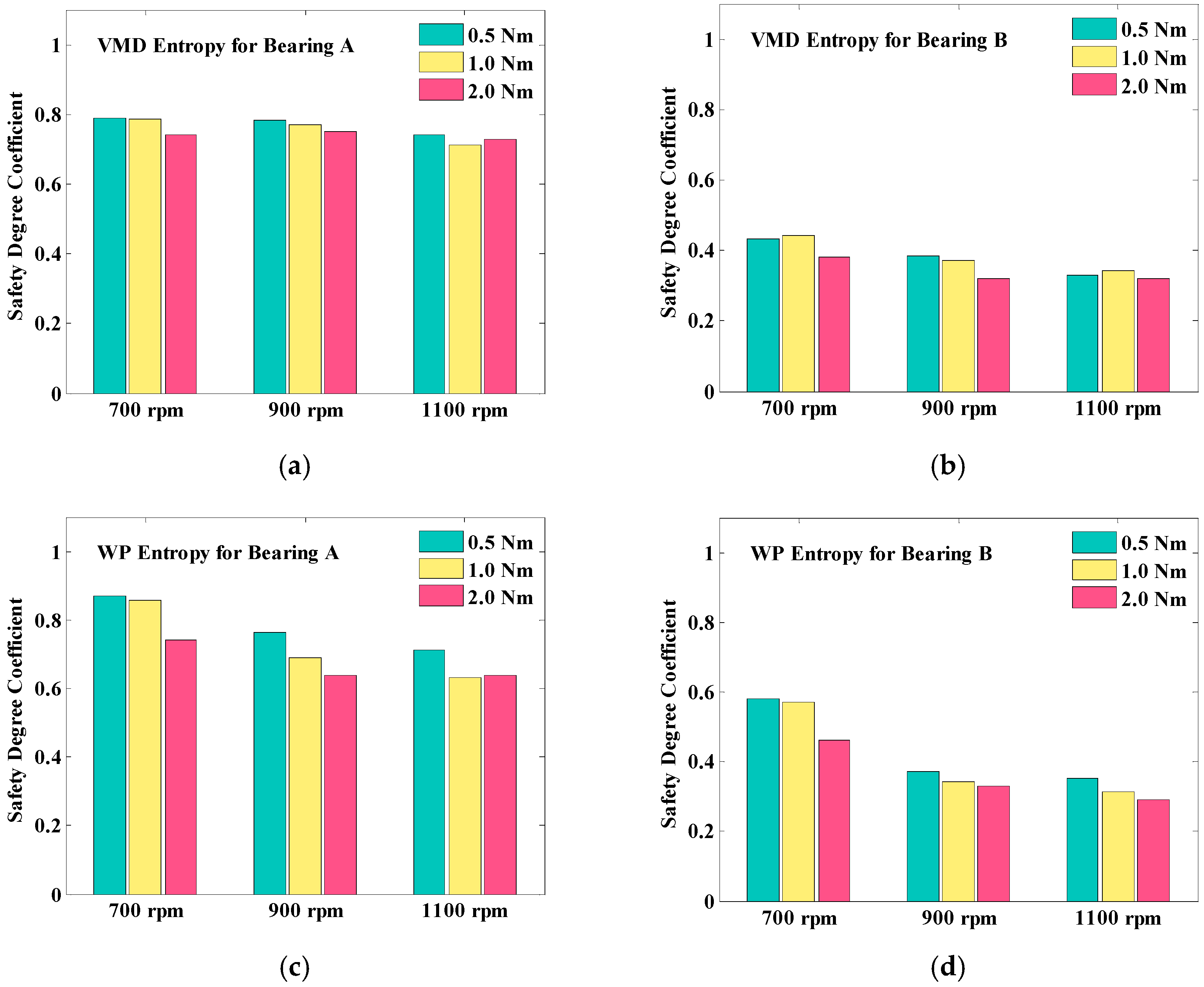
Table 1.
The algorithm steps of variational mode decomposition.
| Step Order | Complete Optimization of VMD |
|---|---|
| Step 1: | Initialize , |
| Step 2: | , n, set values to 0 |
| Step 3: | Update and , based on Equation (13) |
| Step 4: | Update |
| Step 5: | Check Repeat Steps 3 and 4 until the convergence condition |
| Step 6: | End the Decomposition |
Table 2.
Experimental setting and expected defect frequency.
| Setting Operating Condition | Defect Frequency | |
|---|---|---|
| Input Axis Speed | Load Torque | |
| 700 rpm | 0.5 Nm | 120.1 Hz |
| 1.0 Nm | ||
| 2.0 Nm | ||
| 900 rpm | 0.5 Nm | 154.4 Hz |
| 1.0 Nm | ||
| 2.0 Nm | ||
| 1100 rpm | 0.5 Nm | 188.7 Hz |
| 1.0 Nm | ||
| 2.0 Nm | ||
© 2017 by the authors. Licensee MDPI, Basel, Switzerland. This article is an open access article distributed under the terms and conditions of the Creative Commons Attribution (CC BY) license (http://creativecommons.org/licenses/by/4.0/).
Share and Cite
MDPI and ACS Style
Fu, L.; Wei, Y.; Fang, S.; Zhou, X.; Lou, J. Condition Monitoring for Roller Bearings of Wind Turbines Based on Health Evaluation under Variable Operating States. Energies 2017, 10, 1564. https://doi.org/10.3390/en10101564
AMA Style
Fu L, Wei Y, Fang S, Zhou X, Lou J. Condition Monitoring for Roller Bearings of Wind Turbines Based on Health Evaluation under Variable Operating States. Energies. 2017; 10(10):1564. https://doi.org/10.3390/en10101564
Chicago/Turabian StyleFu, Lei, Yanding Wei, Sheng Fang, Xiaojun Zhou, and Junqiang Lou. 2017. "Condition Monitoring for Roller Bearings of Wind Turbines Based on Health Evaluation under Variable Operating States" Energies 10, no. 10: 1564. https://doi.org/10.3390/en10101564
Note that from the first issue of 2016, this journal uses article numbers instead of page numbers. See further details here.