Influence of Dynamic Efficiency in the DC Microgrid Power Balance


Sorbonne University, Université de Technologie de Compiègne, EA7284 Avenues, 60203 Compiègne, France
*
Author to whom correspondence should be addressed.
Energies 2017, 10(10), 1563; https://doi.org/10.3390/en10101563
Submission received: 26 July 2017
/
Revised: 24 September 2017
/
Accepted: 29 September 2017
/
Published: 11 October 2017
(This article belongs to the Section I: Energy Fundamentals and Conversion)
Abstract
:This work aims to enhance the ability of a direct current (DC) microgrid to guarantee the power supply without interruptions by considering the dynamic efficiency of each power converter in the power balance. Previous works show that the converter efficiency varies according to the instant power. If the variable efficiency of the converters in the microgrid is not considered, some extra power must be considered to compensate the losses in the power balance. However, this leads to a waste of available energy and unnecessary load shedding. The work presented here includes the power converters’ dynamic efficiencies in the control of a DC microgrid to improve its performance. MATLAB/Simulink simulations were carried out and the results show that the dynamic efficiency can reduce the load shedding and improve the total DC microgrid efficiency.
1. Introduction
Facing climate change and the public’s awareness of sustainable development, more and more attention has been paid to renewable energy sources. The renewable energy sources, such as photovoltaic (PV) generation and wind turbines, have quite different characteristics from the conventional fossil sources: they are highly variable and intermittent; therefore they cannot directly generate the desired sinusoidal current with a fixed frequency [1]. Thus, besides the high installation cost, there is extra cost to integrate the renewable energy into the conventional electrical power grid, because the needed rapid regulation service is generally provided by natural-gas-fueled power plants. This is one of the main drawbacks of the renewable energy source which limits its penetration in the power grid [2].
In order to resolve these problems, the next-generation power grid, called smart grid, is proposed. Despite the lack of a normalized definition, smart grids are generally believed to have the competence of bidirectional communication and better support for bidirectional power flow [3]. However, the transit from a conventional power grid to a smart-grid can be a long and expensive process. Therefore, a novel distribution technology, the microgrid, can be considered the bridge towards the smart grid. The microgrid aggregates renewable and traditional power generation, storage, and controllable loads at the local level; thus, at the point of common coupling with the power grid, the whole microgrid can be seen as a single element. Due to the storage and controllable loads in the microgrid, the renewable power injected into the grid can be flattened [4].
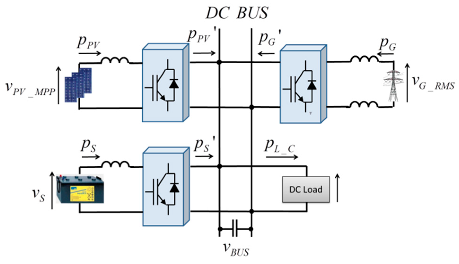
Microgrids can be both alternating current (AC) and DC, depending on the form of the current on the common bus. Noting that the PV generator and the widely applied electrochemical batteries are both native DC components, and the fact that more and more electric equipment can be supplied by DC distribution, the DC microgrid is more energy efficient since it consists of fewer power conversion stages [5]. The simplified architecture of a typical grid-connected DC microgrid is depicted in Figure 1. The renewable energy source, i.e., PV panels, the electrochemical storage, and the AC distribution grid are connected to a common DC bus via dedicated power converters. The loads are also connected to the DC bus, either directly or via their dedicated converters; but, from an energy point of view, the loads and their converters can be seen as a single DC load directly connected on the DC bus. It is noted that νBUS, pPV, pS, pG and pL_C are respectively the common DC bus voltage, the power of the PV source, the electrochemical storage, the power exchanged with the public grid and the constrained load power; and also , and are the powers exchanged with the common bus by the corresponding converters, respectively. More detailed introduction about the variables will be given in Section 3.
As there is no more reactive power and harmonic issues, the power quality of the DC microgrids depends only on the stability of the DC bus voltage. The bus voltage cannot be steady if the power balance inside the microgrid is not well kept [6] and this may lead to power system safety issues and cause more power losses. Therefore, the knowledge of the accurate power flows injected into or withdrawn from the DC bus is important.
In the context of microgrids based on renewable energy, sensors are installed at the output of each source (the input side of each converter), to realize the maximum power point tracking (MPPT), control or monitor the energy use of the storage system and the public grid. However, in most cases no sensors are installed on the output side of the converters, mostly because of the physical constraints (e.g., lack of space in compact converters) or to save on the cost of extra sensors. Thus, the losses in the power converters and the exact power injected into or withdrawn from the DC bus cannot be measured. Furthermore, the efficiency of each power converter is variable, depending on the power, voltage, and the temperature. In this case, accurate knowledge about the power flows on the DC bus is not possible. This problem becomes a key issue in extreme cases, for example when available power supply is not enough for the load power demand and load shedding is necessary. If the power losses are unknown, some extra load power, called safety margin, must be introduced. This safety margin must be large enough to cover the maximal losses of all the power converters but too large a margin will lead to power waste. In order to resolve this problem, the instant power converter loss estimation can be useful to replace or reduce the fixed-value safety margin.
The efficiency of the power converters has been the focus of many research projects for a long time. In [7] a complete converter design procedure was presented, including the choices of the passive and active components, the design of cooling system, and the electromagnetic interference filters. In this procedure, an average power loss estimation method was used to generate the thermal model of the converter, which is essential for the cooling system design. Combining all the physical constraints, a good tradeoff between the efficiency and power density of the converter can be made. A computer-based optimal design procedure of PV inverter was introduced in [8]. The behavioral model of two common types of three phase inverter was established to calculate the power losses of the system. Then, the optimization program would choose the best compromise among the predefined list of semiconductors, inductors, and capacitors, respecting a user-defined weighting function to consider the variable PV power. As well, it is expected to have a good balance between the high efficiency, low cost and high power density.
In [9] a detailed study of the power train efficiency of the electrical vehicle was carried out. It involved the efficiency of the battery, DC/DC converter, inverter, and the motor. This study shows that the global efficiency can be optimized by changing the DC-link voltage and applying different pulse width modulation (PWM) methods. The power loss model is essential for this purpose.
As there are a lot of suitable types of converter for renewable energy applications, the choice must be made according to their performance. In [10] the authors presented the comparison of five non-isolated DC/DC power converters. The state space models were established and the efficiency was analyzed over a large power range. It is noted that the efficiency for a given converter varies according to input power.
Since the power losses of the converter are dissipated in the form of heat, the converter will be heated, and, in turn, the power losses will change too. To take the temperature variation into account, in [11] a precise loss model was proposed with the consideration of the variation of temperature. This model is based on the analysis of the voltage and current waveform during one switching period, so that it is quite precise, but its complexity prevents it from being implemented in real-time systems.
A simple average loss model was used in [12] to estimate the losses in a power converter. The advantage is that it is based on datasheet parameters and the formulas are polynomial, so it can be implemented easily in real-time control systems. Therefore, this average power loss model is applied in this work.
The research works listed above are generally for design and evaluation purposes. However, there are a lot of improvements which can be made by converter efficiency models in real-time control. For example, in [13], a new control method was proposed for an interleaved fly-back converter to improve the efficiency on the low power range. The variable converter efficiency can be used as well to optimize the efficiency of a microgrid if there exist two identical energy storage elements and corresponding converters as stated in [14].
In this work, the instantly efficiency estimation, called dynamic efficiency is presented. This concept will play an important role in the load shedding algorithm and the power control of a DC microgrid. In Section 2, the three load shedding algorithms are introduced. In Section 3, the different load shedding algorithms are compared based on MATLAB/Simulink (The MathWorks, Inc., Natick, MA, USA) simulations. In Section 4, the dynamic efficiency based power converter control is also introduced to improve the microgrid performance. A general conclusion is given in Section 5.
2. Efficiency of the Power Converters in DC Microgrid
In a DC microgrid two kinds of power converters are involved: the DC/DC converter and the DC/AC converter. Their main mission is to interface the sources with the DC bus and to flexibly control the exchanged power. Although a lot of different power converters have been conceived for this purpose, this work studies only the half-bridge DC/DC converter, the full-bridge DC/AC converter and the basic boost converter as illustrated in Figure 2a,b.
The reason is linked to the simplicity of the structure and command, as well as the capability of transferring power in both directions, which is required by the storage and the grid connection. In case of PV panels, there is only unidirectional power flow and the basic boost converter with only one transistor and one diode as shown in Figure 2c is commonly used. When the half bridge DC/DC converter injects energy into the DC bus, it is equivalent to the boost converter and they generate the same amount of power loss. Hence, the loss model of the half bridge DC/DC converter can be also applied to the basic boost converter. The power losses in converters are generated by the semiconductor components and the passive components. The semiconductor losses can be categorized in conduction losses and switching losses, due to the transistors and the diodes respectively. As stated in [15], the copper loss of the inductor is also considered as a main source of power loss. Obviously there are some losses which are not included, such as the core loss of the inductor and the capacitor losses. Some previous research [16,17,18] show that these losses are relatively low compared to the aforementioned major losses so they are neglected in this work.
In [15] an average loss model is used to give a fast and simple estimation of the power losses in the converters in steady state. The estimation is mainly based on the parameters on the datasheet given by the semiconductor manufacturers. The estimated total power loss in a converter, psum_loss, is the sum of five parts: pcondT and pcondD the conduction losses respectively in transistor and diode, pswT and pswD, the switching losses in transistors and diodes, respectively, and pL the copper loss of the inductor.
The formulas of each power loss in the half bridge DC/DC converter are shown in (1):
The voltage drop of the transistor , the voltage drop of the diode , the respective resistances of the transistor and of the diode , the switch-on loss noted and the switch-off loss noted of transistor, and the reverse recovery charge are introduced to describe the semiconductor properties. Among them, the typical values of , , , , and can be found directly on the datasheet. The evolution of and versus the transistor current is also given by the manufacturer (generally, the evolution can be fitted as 2nd order polynomial as ). The other parameters used in (1) are: which is the rated voltage of the semiconductor; which is the switching frequency; which is the duty cycle of converter and for the half bridge DC/DC converter; which is the resistance of the inductor that can be easily measured.
Based on these formulas, the total power loss can be estimated if the source side voltage , bus voltage , and the inductor current are known. Consequently, the instant efficiency can be calculated as follows:
In the case of a single phase full bridge DC/AC converter, the power losses can be estimated in a similar way. However, as the current is AC, modifications must be made. Hence, the formulas for each power loss are as follows:
Besides the parameters introduced before, the formulas include also the average and effective current in the transistor and the diode. These currents can be calculated from the AC current as follows:
where is the modulation index and is the power factor of the AC power. Therefore, the instant efficiency of the DC/AC converter can also be obtained as given by (5).
3. Safety Margin and Dynamic Efficiency
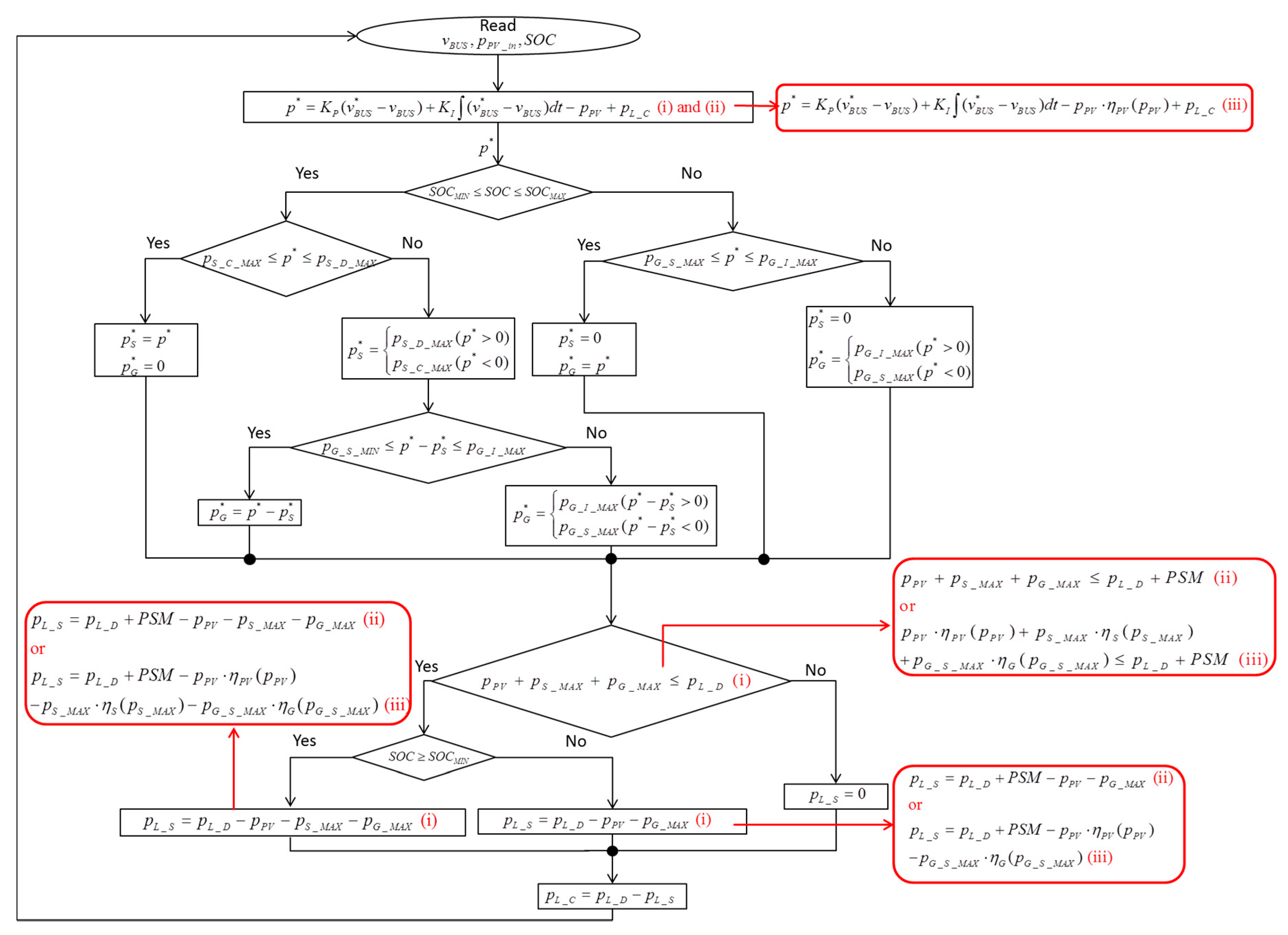
As the solar irradiation is always varying unpredictably and the characteristics of PV panels are nonlinear, a MPPT algorithm is generally used to maximize the PV power generation. Thus, in Figure 1 the PV output power, , is constantly varying; similarly for the constrained load power, , is varying randomly. Hence, the powers of the auxiliary sources, i.e., the storage power, , and the grid power, , are necessary to keep the power balance.
For a DC distribution system, the DC bus voltage is the only indicator of the power quality. Generally, its variation is related to the power balance of the DC microgrid. If the power is well balanced, the bus voltage should be steady within an acceptable fluctuation scope, which is generally ±5% of the DC bus voltage reference . In a previous work [19], without knowledge of the exact injected PV power , the power balance is often realized by applying a voltage loop as follows:
where and are respectively the proportional gain and the integral gain of a proportional-integral (PI) regulator, and is the power reference needed to keep the power balance, i.e., DC bus voltage stabilization. This power reference is then divided into the storage power and grid power references, and , according to the energy management strategy. One popular strategy is the storage-priority strategy, meaning the total power reference will be always assigned to the storage unless the storage is exhausted or exceeds the storage power range.
In order to avoid overdischarging and overcharging, the state of charge noted must be constrained. Moreover, the upper and lower power limits, and , of the storage must be respected to maximize the lifespan of the electrochemical storage. Likewise, the grid power is supposed to be constrained between and , the maximal supply power and the maximal injection power, respectively, either for the physic limits of the devices or for grid operator message via the smart grid communication. In such case, the limited storage and grid power may not meet the need of power balancing, thus a load shedding algorithm is required. The hypothesis in this work is that the load power to be shed pL_S can vary continuously, between zero and 40% of the actual load power demand pL_D. In other words, the total constrained load power pL_C, has a value between 60% and 100% of pL_D.
To balance the power correctly and realize sufficient load shedding, in this study three methods of load shedding are studied. The first one is the classical power balancing, the second one is the power balancing with power safety margin (PSM), and the last one is the power balancing with reduced PSM and dynamic converter efficiency (DCE). All the three methods are depicted in Figure 3.
In this flow the complete classical power balancing procedure is shown by the formulas marked with (i). This method compares simply the reference with the available power of the storage and grid, and then determines the shedding power by the difference. However, this procedure is idealized since it is based on the source powers, such as , , and , instead of the real power arriving at the DC bus, , , and . The difference between the powers on the two sides of each converter is indeed the converter power losses and cannot be neglected even for the high efficiency converters. Therefore, this method often fails to work because it overestimates the available power.
To compensate the converter losses, the second method takes into account some extra consumed power, namely PSM, when comparing and the available power. This can be easily realized by replacing the formulas marked with (i) by those marked with (ii) in Figure 3. However, the sizing of the PSM must be properly made: too high a value leads to unnecessary load shedding and waste of power; a small value can be insufficient to cover all the power losses and avoid the failure of microgrid system. This choice is usually made empirically and mostly as a high value.
As a constant value, PSM should be more than the sum of maximal power losses, but the power converter losses are in fact variable according to the working status of the converters. Unavoidably the PSM method can maintain the safety of power supply but would always cause excessive load shedding. Aiming at more flexible load shedding, the variable efficiency caused by the variable PV generation and load consumption must be considered. Developed in [15], the dynamic efficiency model based on datasheet parameters is suitable for this purpose. Even so, a smaller power safety margin is still needed to compensate the error of estimation. This leads to the third method, the power balancing with reduced PSM and DCE. Based on the instantly measured power of each source, the instant efficiency of each converter, i.e., , and , is estimated and then taken into consideration in the load shedding algorithm, as illustrated in Figure 3 by the formulas marked with (iii). In this third method, the DCE is not only applied to calculate the load power that must be shed, but also influences the calculation of , which lead to more precise power balancing.
4. Simulation Results
For the purpose of comparing the proposed three different power balancing algorithms and to validate the proposed DCE method, simulations under MATLAB/Simulink system were carried out. The simulated microgrid structure is as shown in Figure 1. The parameters of each component are presented in Table 1.
In order to be realistic, real eight-hour PV generation profiles were implemented to simulate the daily DC microgrid operation. Therefore, in this work, the simulated power range is about 1 kW, in order to be compatible with the real PV power profile, and the simulation system parameters are chosen following the test bench presented in [4]. They are also adapted to better fit the presented objectives of the DC microgrid. The energy capacity of the batteries is adapted so that the power cannot exceed 500 W. For the case when the DCE is considered, the PSM is set to be 23 W. Otherwise, it is set to be 85 W. For the safety operation of the DC microgrid, the cut-out of all the sources and the DC load will be taken if the fluctuation of bus voltage exceeds ±5%, meaning allowable bus voltage is between 380 V and 420 V.
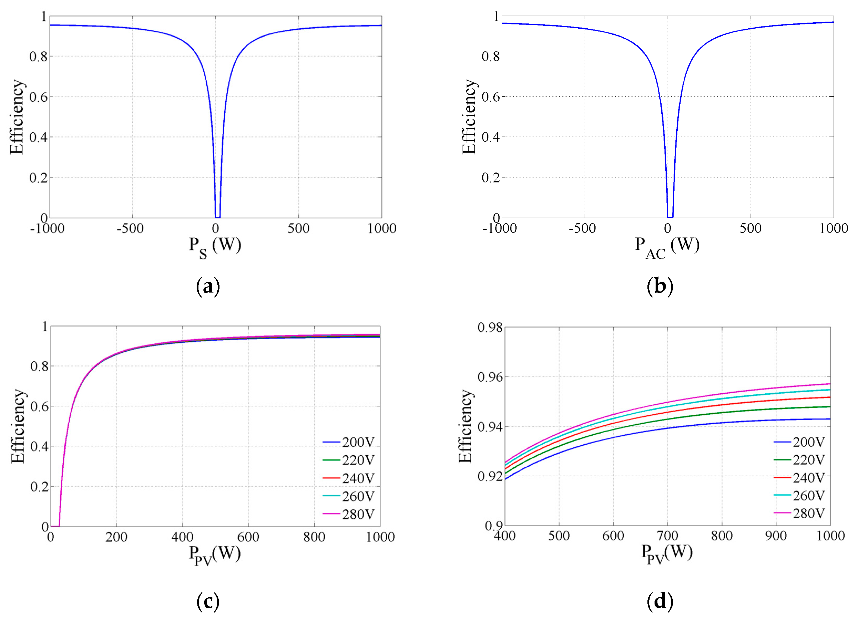
The converter efficiency curves based on the parameters given in Table 1 are shown in Figure 4. Figure 4a,b show that the maximal efficiencies of the converters associated with the storage and grid are both about 96% in the range of 1 kW and the variation of the efficiency is clearly demonstrated by the estimation. It can be noted as well that in a small range of source power above zero, the efficiency keeps at zero. This is because the input power is not more than the generated power loss and output power is zero. Regarding the converter associated with the PV generator, the influence of the input voltage on the efficiency is also given (Figure 4c). Nevertheless, following Figure 4d, it can be concluded that in the scope of 200–280 V the difference of efficiency is really negligible. In addition, as the half bridge DC/DC converter generates the same amount of power loss as the basic Boost converter, the efficiency curve can represent both converters.
4.1. Three Power Balancing Algorithms Comparison
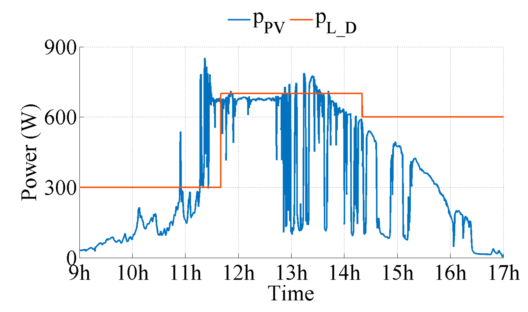
In this first subsection, three algorithms are compared for the same PV MPPT power profile pPV recorded on the 6 November 2014. This day is a typical case of solar irradiation evolution in northern France, which includes relatively high irradiation and the variations caused by clouds. The load power demand profile pL_D is a simplified one to make the analysis easier. These powers are presented in Figure 5.
4.1.1. Classic Power Balancing without Power Safety Margin and No Dynamic Converter Efficiency
Firstly, the classic power balancing without PSM and no DCE is tested. From Figure 6a it is seen that the microgrid has been cut out right before 13:00. This is because the bus voltage has fallen out of the safe range a few minutes before 13 h as shown in Figure 6c. Figure 6b depicts that the lower limit was reached before the failure, so the system relied only on the grid power to keep the power balance. As the grid power is supposed to be limited at 500 W, the output power of grid converter is evidently saturated at a value of less than 500 W.
The zoomed view presented in Figure 6d shows that at the 13854th second, remained 0; since the load shedding algorithm has not been activated before 13855th second, was always keeping 700 W; as the PV power has been decreasing continuously from 276 W to 200 W, consequently and were increasing. However, the load shedding still had not been activated even though arrived at its limit of 500 W and kept still increasing. This is due to the fact that the algorithm ignores the existence of the converter losses and wrongly believed that available power was still enough. Consequently, the bus voltage fell below the safe range and the whole microgrid was shut down.
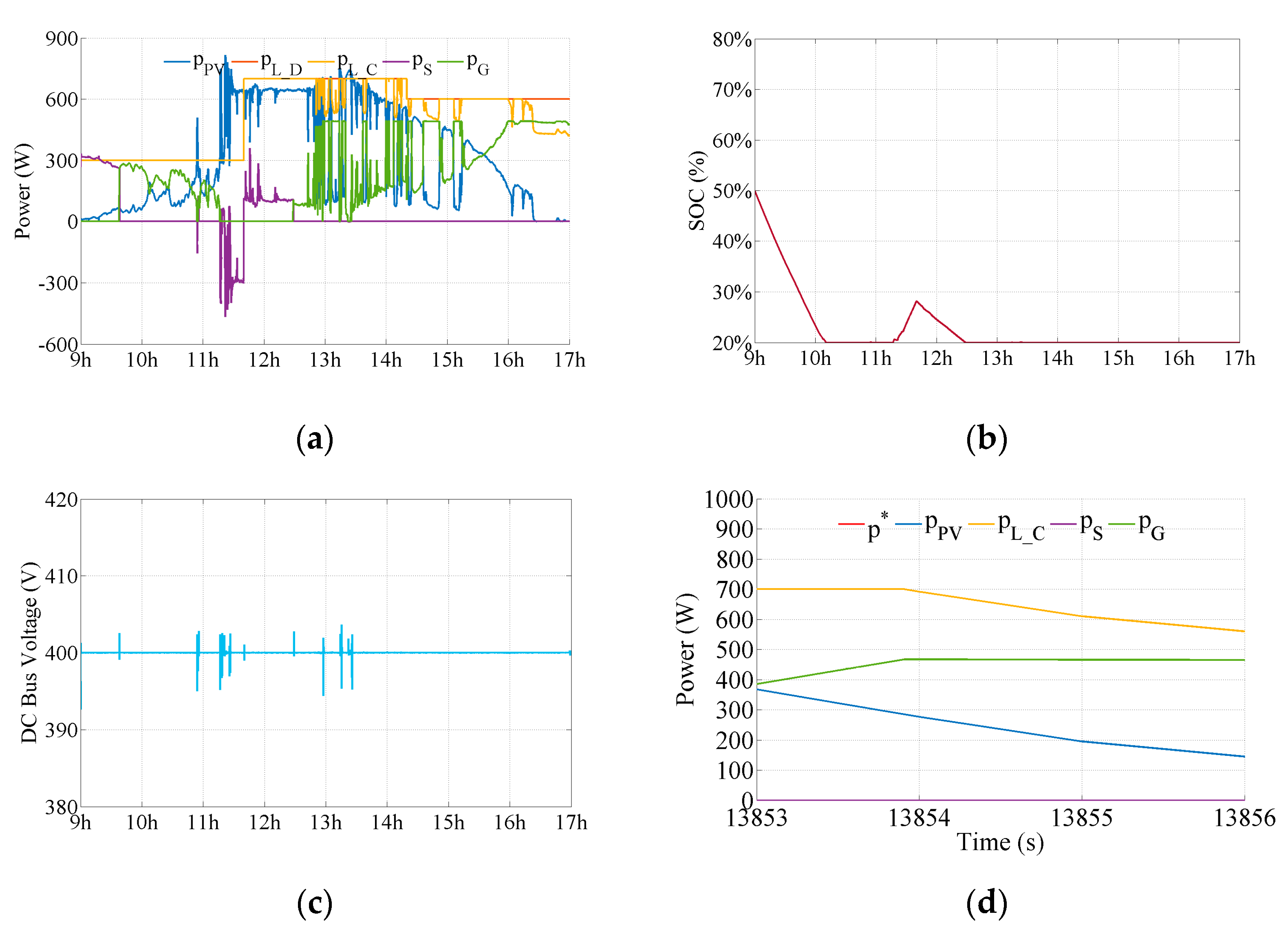
4.1.2. Power Balancing with Power Safety Margin
The second method taking the PSM of 85 W into account is tested with the same profiles. In Figure 7a it is noted the microgrid kept working throughout the eight-hour test, in spite of some bus voltage fluctuations as shown in Figure 7c. The storage has been exhausted since 12h30 as presented in Figure 7b. This time, the bus voltage was steady enough and the microgrid did not stop working because the sufficient PSM activated the load shedding algorithm correctly. It can be seen in Figure 7d that the grid power has never reached the upper limit of 500 W, because of the introduction of PSM. As this PSM is large enough to cover the converter power losses, the load shedding is executed before the saturation of grid power and thus, the bus voltage is kept steady. On one hand, larger this power safety margin becomes, more steady the microgrid would be. On the other hand, a large power safety margin prevents the microgrid from taking full advantage of the potential of energy storage system and grid connection. Moreover, some load power would be shed unnecessarily. It can be expected to approach the source power to their limits and avoid oversizing the sources by minimizing the PSM. But a good compromise between minimizing the PSM and guaranteeing the continuous operation of microgrid can hardly be made in practice unless the converter power losses are well known.
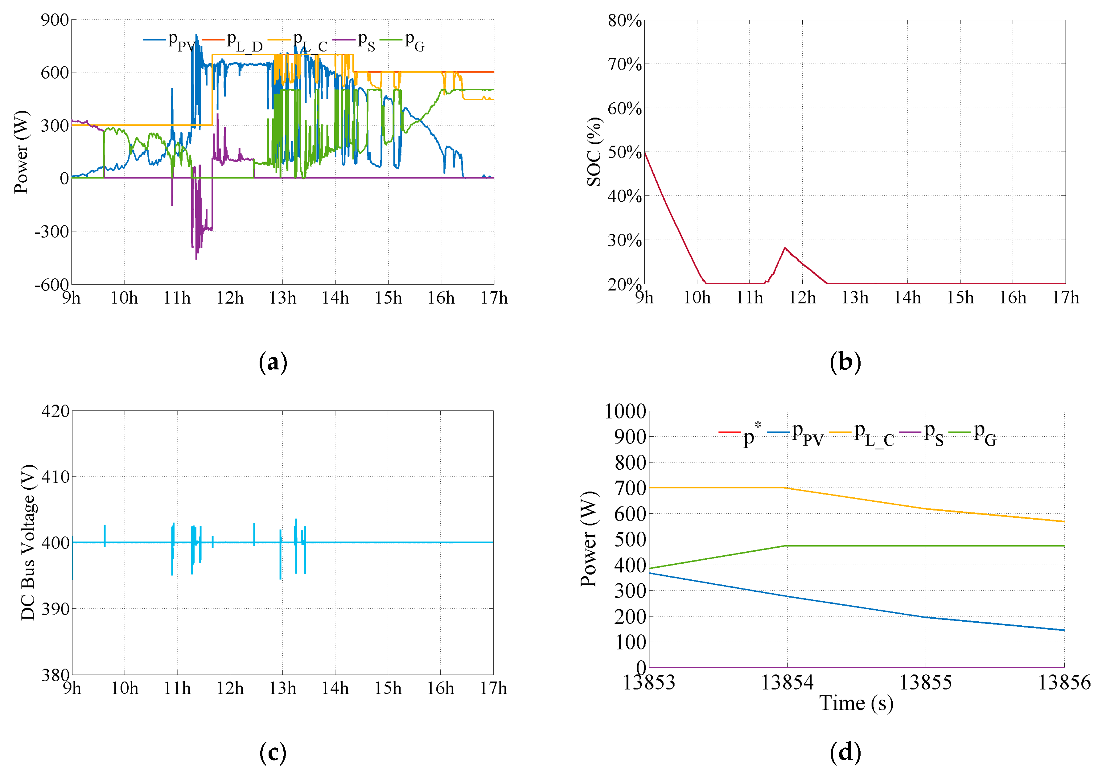
4.1.3. Power Balancing with Power Safety Margin and Dynamic Converter Efficiency
The third method makes the microgrid steady enough even though the safety margin has decreased by 73%, from 85 W to 23 W. This proves that the system has a better knowledge of the power flows. The results shown in Figure 8 can hardly be distinguished from those in Figure 7 because the difference is not at visible at this scale. Some numerical analyses are needed to study the improvements brought by this third algorithm.
To compare bus voltage fluctuation, the standard deviation of the bus voltage is a simple and representative indicator. Concerning the energy performance of the whole microgrid, the averaged global efficiency, defined as , can be utilized.
To evaluate the performance of the microgrid, a virtual microgrid operation cost is proposed according to [20]. Aiming at showing the impacts of the different load shedding algorithms on the energy cost, the total energy cost should be calculated as follows:
where , , and are the energy prices for storage power, grid power, and the virtual price of load shedding, respectively.
The prices are set as in Equation (8) to reflect the high penalization of the load shedding:
The aforementioned numerical indicators are shown in Table 2. The total load energy demand was 4.2667 kWh whilst the load consumed energy was always less due to the partly load shedding. Therefore, Table 2 shows that the load demand was better satisfied in the case of power balancing with DCE and smaller power safety margin. Some other indicators are also chosen to reflect the performance of the microgrid system, such as the global efficiency , the standard deviation of bus voltage as the indicator of fluctuation of the DC bus voltage. Except the classical power balancing which lacks the needed stability, it is concluded that the two other methods of power balancing have little influence on both the global efficiency and the standard deviation of bus voltage of the microgrid. As analyzed before, the DCE reduces the load shedding while still keeping the system stability. Thus, the third method had less total energy cost as the load shedding price was taken into account.
4.2. Tests on Different Day Profiles
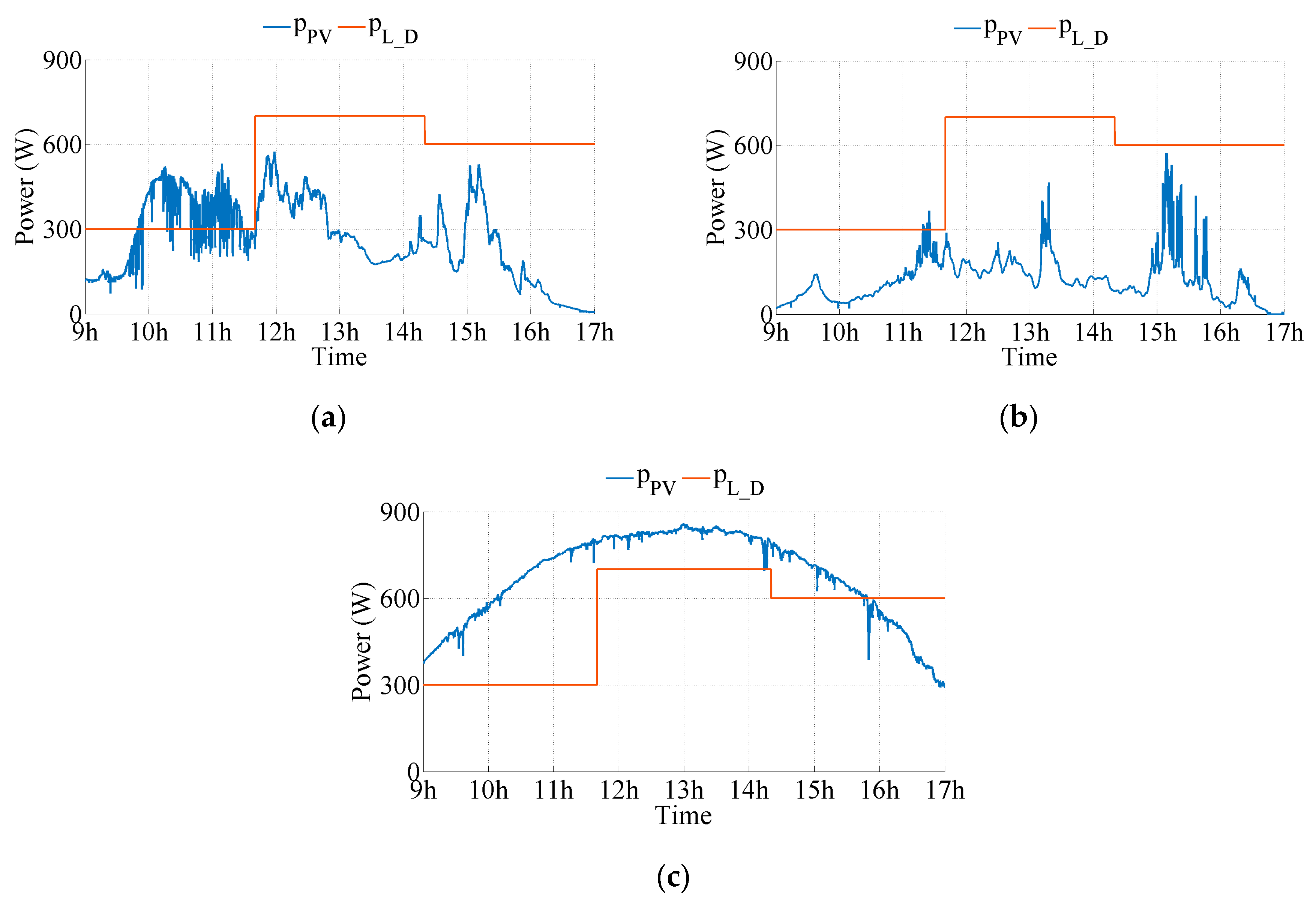
To test the effectiveness of the proposed method in more general scenarios, the simulation of microgrid is tested on three different PV power generation profiles, which are illustrated in Figure 9. They are representative respectively for the cases of: moderate solar irradiation, weak solar irradiation, and strong solar irradiation almost without clouds. The load power demand profile is as same as presented in Figure 5.
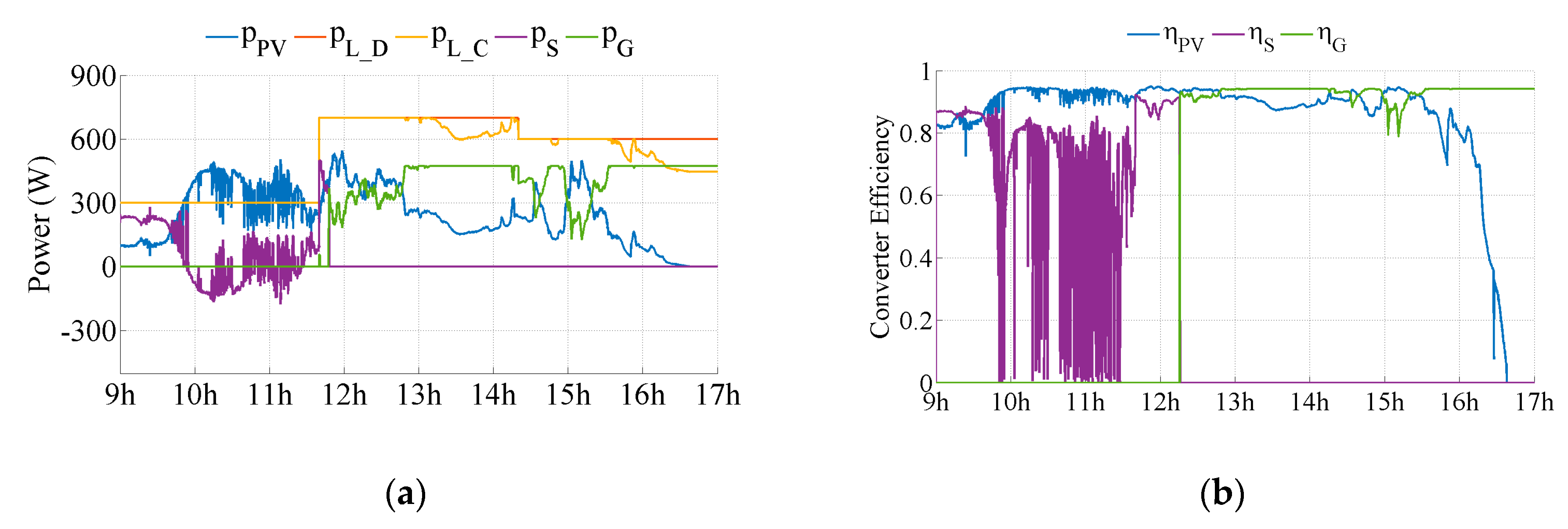
As aforementioned, the classical power balancing without PSM and DCE was still not steady enough, thus only the other two algorithms were tested. The PSM maintains 85 W and 23 W respectively for all the three days to simplify the comparison. With these values, both algorithms succeeded in avoiding failure during all the three days. Considering the similarity of the figures, only the curves of powers evolution and the curves of the converters efficiency evolution of the last method (DCE) are shown in Figure 10.
Figure 10a,c,e show that the load shedding is highly dependent on the PV production. For example, on 27 January 2014, a day when the solar irradiation is obviously low, the load has been severely shed. On the contrary, on 12 March 2015, there was almost no load shedding because of excessive PV power. Figure 10b,d,f demonstrate that the efficiency of the PV converter depends on the PV power as well. On the first and last day, the PV converter worked constantly with high efficiency, except for the end of the day. But on 27 January 2015 the efficiency was highly variable and it should not be treated as a constant. Concerning the power converters of the storage and the grid, the situation is more complicated since the auxiliary source power depends on both the available PV power and load power demand. No matter whether there was a lot of or just a little PV power, the storage and grid associated converters invariably worked with relatively low efficiency for some time. This fact justifies the introduction of DCE in the control of microgrid.
Taking into account the variation of converter efficiencies during the studied period, it is obvious that the global efficiency of the DC microgrid has also some fluctuation. Figure 11 shows the evolution of instant global efficiency, defined as , for the DCE method. It can be seen clearly that the global efficiency does not have a direct relation with PV profile. The fluctuation of the blue curve was evidently caused by the fluctuation of PV power, but the highest PV power on the 12 March 2015 did not correspond to the highest global efficiency. On the contrary, during some period, this day has the lowest global efficiency. This implies that the improvement of the global efficiency may need optimization of power flow dispatching in the microgrid with prediction of PV power generation and load power demand.
In Table 3 the numeric results of the three days are listed. It can be seen that the two methods, PSM and DCE, had nearly no difference in the global efficiency and the fluctuation of . On the contrary, they made a difference on the total consumed energy and total operation cost. The negative cost of the third day means the energy cost of the microgrid was less than the benefits of supplying the grid. The difference mainly lays on the energy consumed by the load. The day with least PV power has the highest energy cost due to the frequent load shedding. The comparison of the two methods illustrates the DCE can effectively reduce the load shedding thus reducing the energy cost, particularly in the days with less PV power.
5. Dynamic Converter Efficiency in Power Balancing and Power Control
The estimation of converter efficiency cannot only be implemented in power balancing algorithm, but also it can be used in local power control loop of storage and grid. In the precedent sections, the outer voltage control loop of the microgrid can be represented by Figure 12.
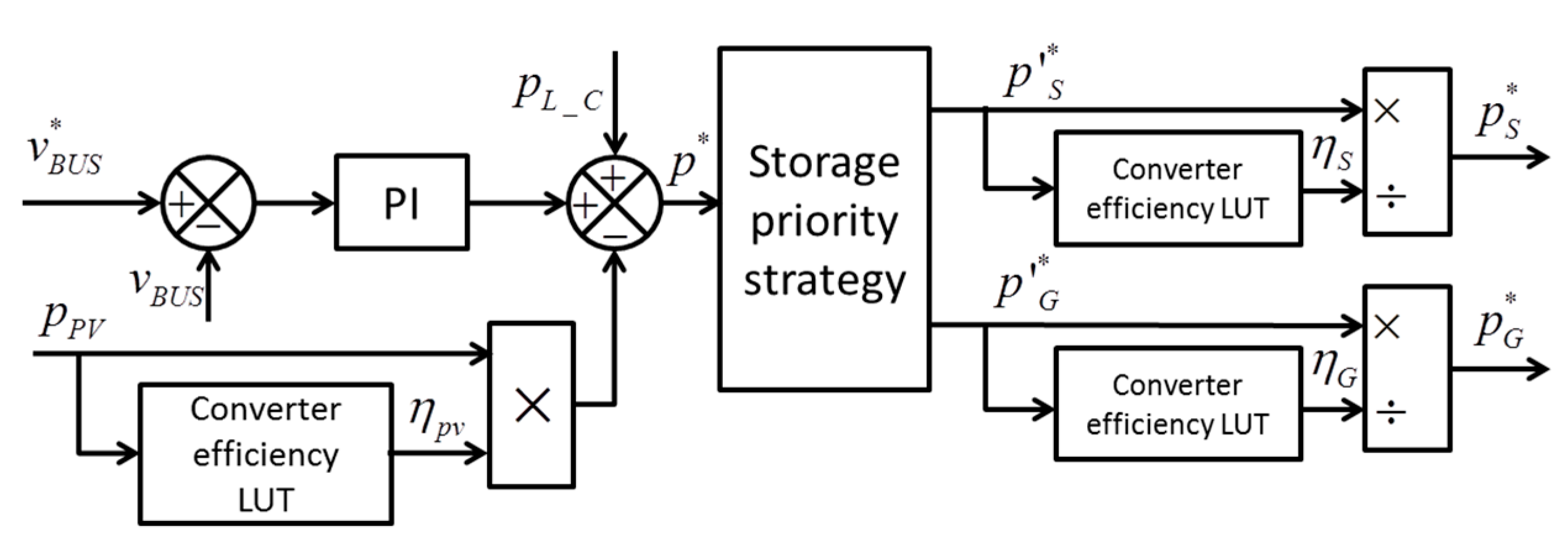
In this way, the total power reference is divided into two parts and , according to the storage priority strategy. However, as stated in Section 4, the strategy does not consider the power losses and it depends on the robustness of the regulator to compensate the power losses. As a result, the process of the convergence will lead to more bus voltage oscillations, thus the power quality is degraded. In order to accelerate the convergence and improve the power quality of the DC microgrid, a feed-forward method based on estimation of efficiency can be introduced in the control loop. Thus, the following loop is implemented instead of the one above (Figure 13).
Adapted to the high frequency execution of the regulation system, the converter efficiency estimation is implemented in form of a Look-up Table, which has the power and voltage as input and the converter efficiency as the output. In this way, the generated power references and contain both the required power and the instant power losses so that the convergence would be accelerated. To prove this, the tests based on the four aforementioned PV power profiles were carried out to compare the three methods: the two methods presented before and a new one which integrate the DCE method and the dynamic efficiency power control (DEPC). The results are shown in Table 4.
From this comparison one can note the DEPC has a complex performance. Except for the last day that had almost no drastic PV power variation, on the other three days this method helped to reduce the DC bus voltage fluctuation, at the expense of slightly decreasing system global efficiency and increasing the energy cost somewhat. In particular, on the day of 27 January 2015 whose PV power generation was weak, the DEPC method improved the global efficiency by 2.3%, signifying this method allowed the DC microgrid to correctly treat the PV converter losses. On the contrary, the DEPC only had negative effects on the day of 12 March 2015. It is because the PV converter worked with nearly constant efficiency and in this case the DEPC method had added unnecessary power fluctuation. From this comparison, it is obvious that the DEPC method can play an important role on the days when solar irradiation is highly variable and weak, which happens often in some regions such as northern France.
6. Conclusions
To ensure the power quality of a DC microgrid, the power balance method including load shedding is essential. Different power balancing methods are proposed and tested in simulation. It is proved that the power balancing cannot work without an appropriate PSM. The dynamic efficiency estimation enables the system to know better the power losses in the microgrid thus making more flexible and precise load shedding. The simulation tests based on different real PV profiles prove it. The dynamic efficiency estimation is also proposed to help treat the converter power loss by changing the power control loop. According to the simulations this method helps reduce the bus voltage fluctuation but increases energy costs on cloudy days. The power range of the simulation can be easily scaled up to a few 100 kW to show more obvious economic benefits, but the conclusions will not be changed compared to the chosen low power range. In future work progress can be made by optimizing the power flow dispatching in the microgrid with consideration of power losses to improve the global efficiency.
Author Contributions
All authors have designed the system, performed the simulations, and analyzed the data. All authors contributed jointly to the writing and preparing revision of this manuscript. All authors have read and approved the manuscript.
Conflicts of Interest
The authors declare no conflict of interest.
References
- Wang, H.; Blaabjerg, F.; Simões, M.G.; Yang, Y. Power control flexibilities for grid-connected multi-functional photovoltaic inverters. IET Renew. Power Gener. 2016, 10, 504–513. [Google Scholar] [CrossRef]
- Liang, X. Emerging Power Quality Challenges Due to Integration of Renewable Energy Sources. IEEE Trans. Ind. Appl. 2017, 53, 855–866. [Google Scholar] [CrossRef]
- Molderink, A.; Bakker, V.; Bosman, M.G.C.; Hurink, J.L.; Smit, G.J.M. Management and control of domestic smart grid technology. IEEE Trans. Smart Grid 2010, 1, 109–119. [Google Scholar] [CrossRef]
- Sechilariu, M.; Wang, B.; Locment, F. Building Integrated Photovoltaic System With Energy Storage and Smart Grid Communication. IEEE Trans. Ind. Electron. 2013, 60, 1607–1618. [Google Scholar] [CrossRef]
- Wu, H.; Sechilariu, M.; Locment, F. Impact of power converters’ efficiency on building-integrated microgrid. In Proceedings of the 17th European Conference on Power Electronics and Applications (EPE’15 ECCE-Europe), Geneva, Switzerland, 8–10 September 2015; pp. 1–10. [Google Scholar]
- Wu, T.F.; Chang, C.H.; Lin, L.C.; Yu, G.R.; Chang, Y.R. DC-bus voltage control with a three-phase bidirectional inverter for DC distribution systems. IEEE Trans. Power Electron. 2013, 28, 1890–1899. [Google Scholar] [CrossRef]
- Wen, B.; Boroyevich, D.; Mattavelli, P. Investigation of tradeoffs between efficiency, power density and switching frequency in three-phase two-level PWM boost rectifier. In Proceedings of the 2011 14th European Conference on Power Electronics and Applications (EPE’11 ECCE-Europe), Birmingham, UK, 30 August–1 September 2011; pp. 1–10. [Google Scholar]
- Pinne, J.; Gruber, A.; Rigbers, K.; Sawadski, E.; Napierala, T. Optimization and comparison of two three-phase inverter topologies using analytic behavioural and loss models. In Proceedings of the IEEE Energy Conversion Congress and Exposition (ECCE), Raleigh, NC, USA, 15–20 September 2012; pp. 4396–4403. [Google Scholar]
- Stempfle, M.; Fischer, M. Loss modelling to optimize the overall drive train efficiency. In Proceedings of the 17th European Conference on Power Electronics and Applications (EPE’15 ECCE-Europe), Geneva, Switzerland, 8–10 September 2015; pp. 1–10. [Google Scholar]
- Sivakumar, S.; Sathik, M.J.; Manoj, P.S.; Sundararajan, G. An assessment on performance of DC-DC converters for renewable energy applications. Renew. Sustain. Energy Rev. 2016, 58, 1475–1485. [Google Scholar] [CrossRef]
- Tang, Y.; Ma, H. An Improved Analytical IGBT Model for Loss Calculation Including Junction Temperature and Stray Inductance. In Proceedings of the IEEE 24th International Symposium on Industrial Electronics (ISIE), Buzios, Brazil, 3–5 June 2015; pp. 227–232. [Google Scholar]
- Lana, A.; Mattsson, A.; Nuutinen, P.; Peltoniemi, P.; Kaipia, T.; Kosonen, A.; Aarniovuori, L.; Partanen, J. On Low-Voltage DC Network Customer-End Inverter Energy Efficiency. IEEE Trans. Smart Grid 2014, 5, 2709–2717. [Google Scholar] [CrossRef]
- Kim, Y.H.; Ji, Y.H.; Kim, J.G.; Jung, Y.C.; Won, C.Y. A new control strategy for improving weighted efficiency in photovoltaic AC module-type interleaved flyback inverters. IEEE Trans. Power Electron. 2013, 28, 2688–2699. [Google Scholar] [CrossRef]
- Meng, L.; Dragicevic, T.; Vasquez, J.C.; Guerrero, J.M. Tertiary and Secondary Control Levels for Efficiency Optimization and System Damping in Droop Controlled DC-DC Converters. IEEE Trans. Smart Grid 2015, 6, 2615–2626. [Google Scholar] [CrossRef]
- Wu, H.; Sechilariu, M.; Locment, F. Operation of a photovoltaic-based DC microgrid with consideration of dynamic efficiency of converters. In Proceedings of the 12th ELECTRIMACS International Conference (ELECTRIMACS 2017), Toulouse, France, 4–6 July 2017; pp. 1–6. [Google Scholar]
- Schirone, L.; Macellari, M. Loss Analysis of Low-Voltage TLNPC Step-Up Converters. IEEE Trans. Ind. Electron. 2014, 61, 6081–6090. [Google Scholar] [CrossRef]
- Chen, Z.; Liu, S.; Shi, L.; Ji, F. Power loss analysis and comparison of two full-bridge converters with auxiliary networks. IET Power Electron. 2012, 5, 1934–1943. [Google Scholar] [CrossRef]
- Guo, Z.; Sun, K.; Zhang, L. Analysis and Evaluation of Dual Half-Bridge Cascaded Three-Level DC-DC Converter for Reducing Circulating Current Loss. IEEE J. Emerg. Sel. Top. Power Electron. 2017, 5, 351–362. [Google Scholar] [CrossRef]
- Locment, F.; Sechilariu, M.; Houssamo, I. DC Load and Batteries Control Limitations for Photovoltaic Systems. Experimental Validation. IEEE Trans. Power Electron. 2012, 27, 4030–4038. [Google Scholar] [CrossRef]
- Santos, L.T.D.; Sechilariu, M.; Locment, F. Prediction-based economic dispatch and online optimization for grid-connected DC microgrid. In Proceedings of the IEEE International Energy Conference (ENERGYCON), Leuven, Belgium, 4–8 April 2016; pp. 1–6. [Google Scholar]
Figure 1.
DC microgrid architecture.

Figure 2.
(a) Half bridge DC/DC converter; (b) Full bridge DC/AC converter (c) Basic Boost DC/DC converter.
Figure 2.
(a) Half bridge DC/DC converter; (b) Full bridge DC/AC converter (c) Basic Boost DC/DC converter.
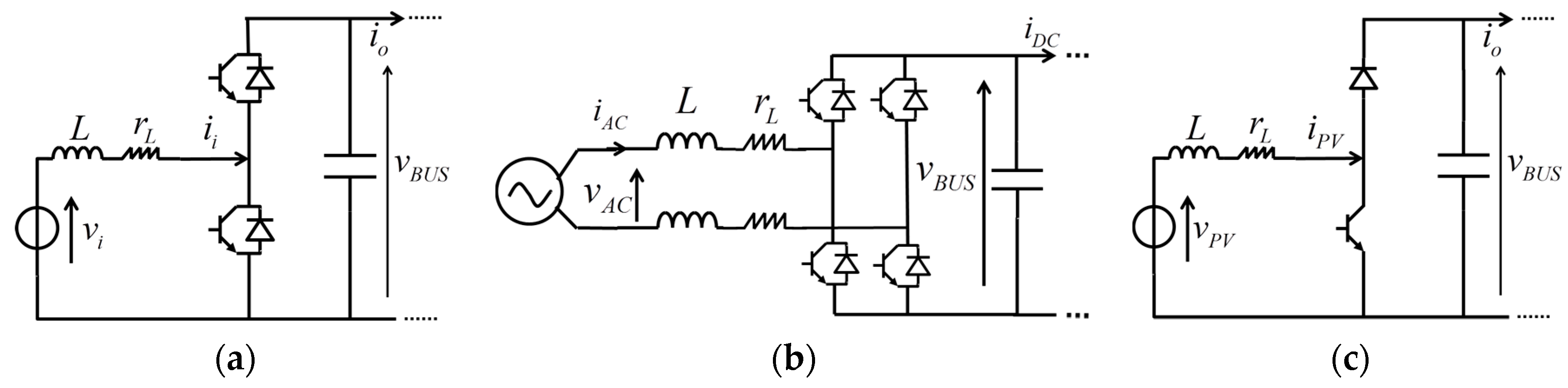
Figure 3.
Power balancing flowchart.

Figure 4.
Converter efficiency curve obtained by the estimation: (a) half bridge DC/DC converter efficiency versus storage power; (b) full bridge DC/AC converter efficiency versus grid power when ; (c) half bridge DC/DC converter efficiency versus PV power for different PV generator voltages; (d) zoomed view of PV converter efficiency for different PV generator voltages.

Figure 5.
PV power profile of 6 November 2014 and load power profile.

Figure 6.
Classical power balancing: (a) evolution of each microgrid power; (b) SOC evolution; (c) bus voltage evolution; (d) zoomed view of powers when the microgrid fails.
Figure 6.
Classical power balancing: (a) evolution of each microgrid power; (b) SOC evolution; (c) bus voltage evolution; (d) zoomed view of powers when the microgrid fails.
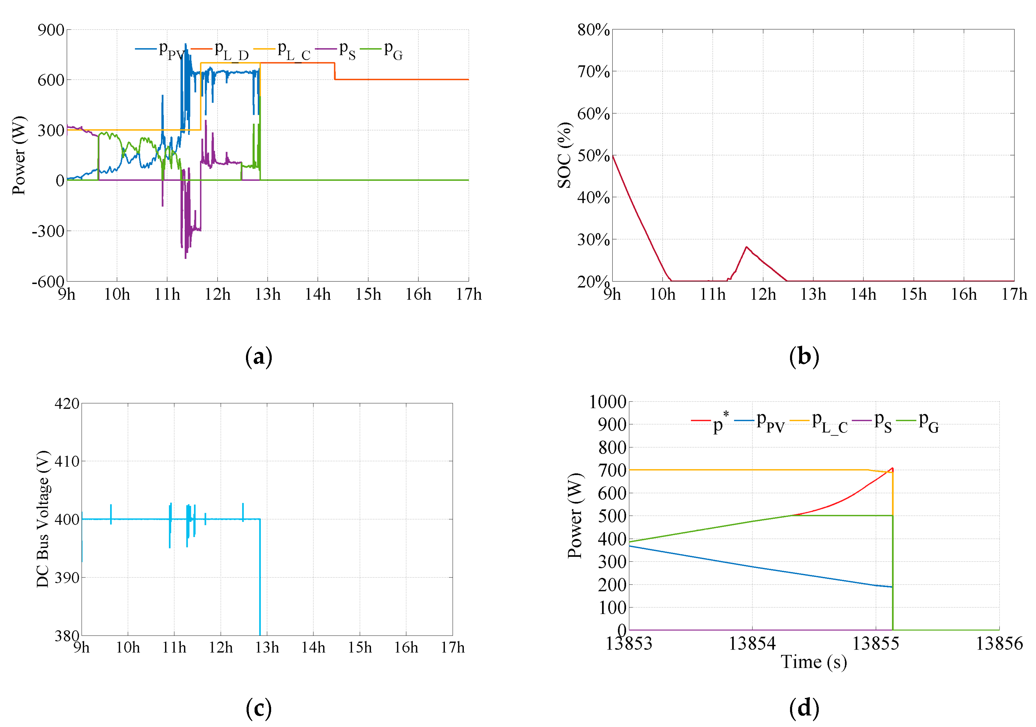
Figure 7.
Power balancing with PSM: (a) evolution of each microgrid power; (b) SOC evolution; (c) bus voltage evolution; (d) zoomed view of power at the time when microgrid failed in first test.
Figure 7.
Power balancing with PSM: (a) evolution of each microgrid power; (b) SOC evolution; (c) bus voltage evolution; (d) zoomed view of power at the time when microgrid failed in first test.

Figure 8.
Power balancing with DCE and smaller PSM: (a) evolution of each microgrid power; (b) SOC evolution; (c) bus voltage evolution; (d) zoomed view of power at the time when microgrid failed in first test.
Figure 8.
Power balancing with DCE and smaller PSM: (a) evolution of each microgrid power; (b) SOC evolution; (c) bus voltage evolution; (d) zoomed view of power at the time when microgrid failed in first test.

Figure 9.
PV and load power profiles: (a) PV power profile of 13 November 2014; (b) PV power profile of 27 January 2015; (c) PV power profile of 12 March 2015.
Figure 9.
PV and load power profiles: (a) PV power profile of 13 November 2014; (b) PV power profile of 27 January 2015; (c) PV power profile of 12 March 2015.

Figure 10.
Power balancing with DCE and smaller PSM: (a) powers evolution and (b) DCE power for 13 November 2014; (c) powers evolution and (d) DCE power for 27 January 2015; (e) powers evolution and (f) DCE power for 12 March 2015.
Figure 10.
Power balancing with DCE and smaller PSM: (a) powers evolution and (b) DCE power for 13 November 2014; (c) powers evolution and (d) DCE power for 27 January 2015; (e) powers evolution and (f) DCE power for 12 March 2015.

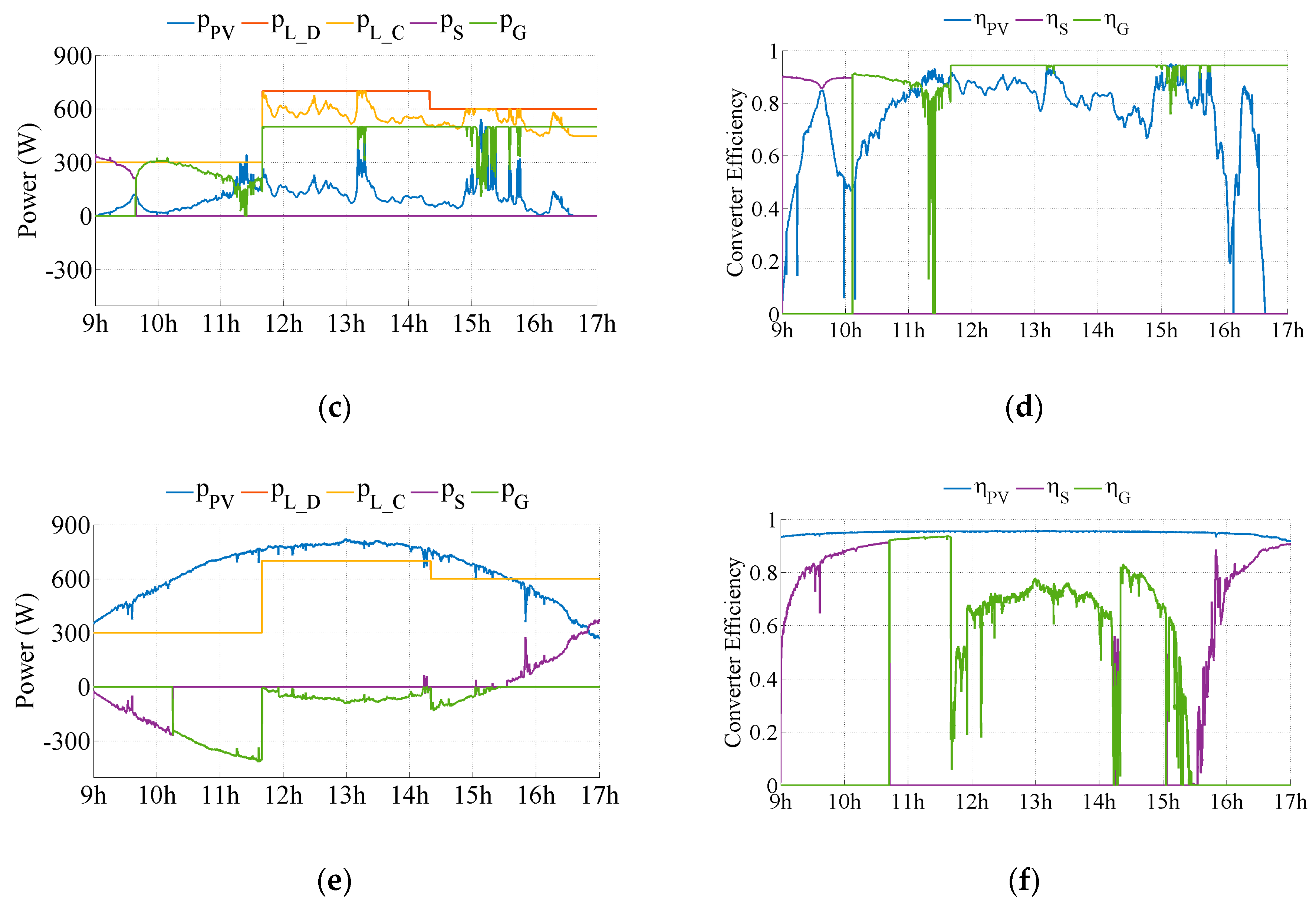
Figure 11.
Comparison of the DC microgrid global efficiencies of the three days for DCE method.
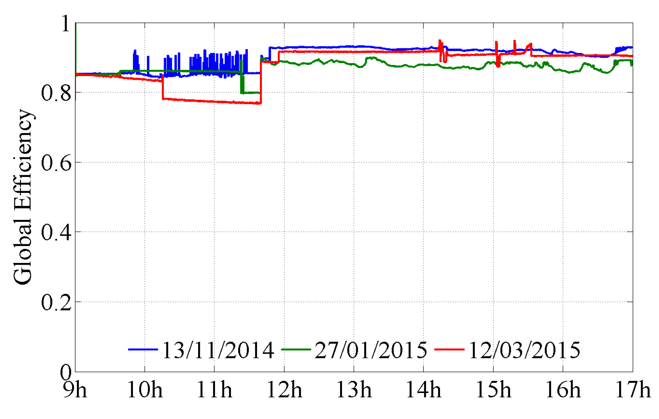
Figure 12.
Control loop without DCE.
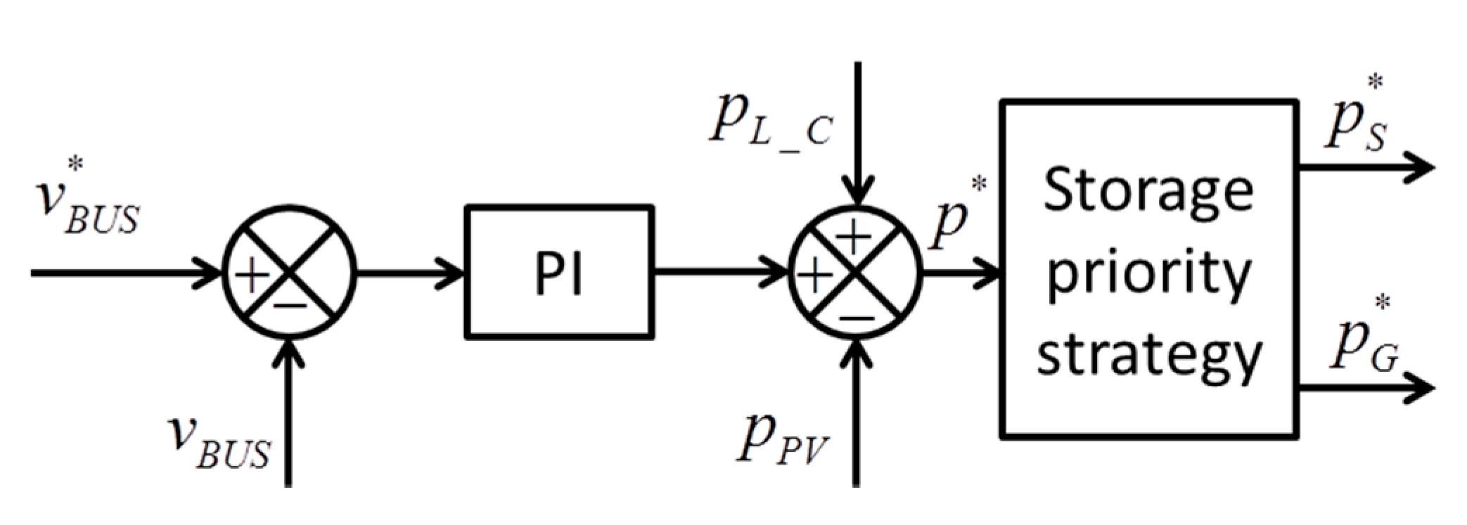
Figure 13.
Improved control loop with converter efficiency estimation.

Table 1.
Simulation system parameters.
| Component | Parameters |
|---|---|
| PV Panels | Maximum power under standard condition tests: 140 V, 7.14 A, 1000 W (Solar-Fabrik, SF 130/2-125, Freiburg, Germany) |
| Batteries | 240 V, 1.35 Ah, power limited to 500 W |
| Grid | Single phase 230 V RMS AC, power limited to 500 W |
| Semiconductor switch + driver | SKM100GB063D + SKH22A (SEMIKRON, Nürnberg, Germany) |
| DC Bus voltage reference | 400 V |
| Bus capacitor | 2200 μF |
| Inductor for PV and batteries | 50 mH, 0.2 Ω |
| Inductor for grid | 40 mH, 0.2 Ω |
| Switching frequency | 10 kHz |
| SOC limits | 20–80% |
| Safe bus voltage fluctuations interval | 380 V–420 V |
Table 2.
Comparison of the three methods.
| Method | PSM (W) | Stability | (V) | (kWh) | (c€) | |
|---|---|---|---|---|---|---|
| Classical | 0 | No | - | - | - | - |
| PSM | 85 | Yes | 0.078 | 4.0562 | 49.95 | 88.06% |
| DCE | 23 | Yes | 0.075 | 4.0736 | 47.56 | 88.02% |
Table 3.
Comparison of the last two methods for the three considered days.
| Date | Method | PSM (W) | (V) | (W) | (c€) | |
|---|---|---|---|---|---|---|
| 13 November 2014 | PSM | 85 | 0.123 | 4.0117 | 58.39 | 90.83% |
| DCE | 23 | 0.119 | 4.0386 | 54.63 | 90.88% | |
| 27 January 2015 | PSM | 85 | 0.046 | 3.6744 | 118.28 | 87.21% |
| DCE | 23 | 0.039 | 3.7214 | 111.70 | 87.34% | |
| 12 March 2015 | PSM | 85 | 0.070 | 4.2667 | −5.83 | 89.12% |
| DCE | 23 | 0.064 | 4.2667 | −5.80 | 88.99% |
Table 4.
Comparison of the three methods for the four considered days.
| Date | Method | PSM (W) | (V) | (W) | (c€) | |
|---|---|---|---|---|---|---|
| 6 November 2014 | DCE | 23 | 0.074 | 4.0736 | 46.29 | 88.09% |
| DCE + DEPC | 23 | 0.060 | 4.0682 | 47.12 | 87.93% | |
| 13 November 2014 | DCE | 23 | 0.119 | 4.0386 | 54.63 | 90.88% |
| DCE + DEPC | 23 | 0.117 | 4.0282 | 56.52 | 89.97% | |
| 27 January 2015 | DCE | 23 | 0.039 | 3.7214 | 111.70 | 87.34% |
| DCE + DEPC | 23 | 0.024 | 3.7026 | 113.22 | 89.63% | |
| 12 March 2015 | DCE | 23 | 0.064 | 4.2667 | −5.80 | 88.99% |
| DCE + DEPC | 23 | 0.083 | 4.2667 | −5.42 | 88.32% |
© 2017 by the authors. Licensee MDPI, Basel, Switzerland. This article is an open access article distributed under the terms and conditions of the Creative Commons Attribution (CC BY) license (http://creativecommons.org/licenses/by/4.0/).
Share and Cite
MDPI and ACS Style
Wu, H.; Sechilariu, M.; Locment, F. Influence of Dynamic Efficiency in the DC Microgrid Power Balance. Energies 2017, 10, 1563. https://doi.org/10.3390/en10101563
AMA Style
Wu H, Sechilariu M, Locment F. Influence of Dynamic Efficiency in the DC Microgrid Power Balance. Energies. 2017; 10(10):1563. https://doi.org/10.3390/en10101563
Chicago/Turabian StyleWu, Hongwei, Manuela Sechilariu, and Fabrice Locment. 2017. "Influence of Dynamic Efficiency in the DC Microgrid Power Balance" Energies 10, no. 10: 1563. https://doi.org/10.3390/en10101563
Note that from the first issue of 2016, this journal uses article numbers instead of page numbers. See further details here.