Estimating the Value of Price Risk Reduction in Energy Efficiency Investments in Buildings

1
VTT Technical Research Centre of Finland Ltd., P.O. Box 1000, 02044 VTT Espoo, Finland
2
OP Financial Group, P.O. Box 308, 00101 Helsinki, Finland
*
Author to whom correspondence should be addressed.
Energies 2017, 10(10), 1545; https://doi.org/10.3390/en10101545
Submission received: 31 August 2017
/
Revised: 21 September 2017
/
Accepted: 3 October 2017
/
Published: 8 October 2017
Abstract
:This paper presents a method for calculating the value of price risk reduction to a consumer that can be achieved with investments in energy efficiency. The value of price risk reduction is discussed to some length in general terms in the literature reviewed but, so far, no methodology for calculating the value has been presented. Here we suggest such a method. The problem of valuating price risk reduction is approached using a variation of the Black–Scholes model by considering a hypothetical financial instrument that a consumer would purchase to insure herself against unexpected price hikes. This hypothetical instrument is then compared with an actual energy efficiency investment that reaches the same level of price risk reduction. To demonstrate the usability of the method, case examples are calculated for typical single-family houses in Finland. The results show that the price risk entailed in household energy consumption can be reduced by a meaningful amount with energy efficiency investments, and that the monetary value of this reduction can be calculated. It is argued that this often-overlooked benefit of energy efficiency investments merits more consideration in future studies.
1. Introduction
This paper presents a method for calculating the value of price risk reduction that can be achieved with investments in energy efficiency by an energy consumer. The main aim of this paper is to show how such a calculation could be done in principle, while the complexities of the problem will require more development work in the future. The value of price risk reduction is largely overlooked so far in literature concerning the costs and benefits of energy efficiency in buildings. While the topic is discussed to some length in general terms in the literature reviewed for this paper, no methodology for calculating the value was presented. Here we suggest such a method with some preliminary results from case examples.
The calculation examples presented in this paper deal with buildings and electricity for heating, but the principles can as well be applied to other contexts. The calculations presented concentrate on heating energy only because there it is relatively easy to find examples of investments that reduce energy consumption, making it well suited for demonstrating the issues at hand. Moreover, they concentrate on electricity as an energy carrier, as volatility data is needed and there is a relatively well functioning electricity market in the Nordic countries. In many cases there is still strong regulation in energy prices but electricity in Nordic countries has had a market price since the 1990s thus providing a rich source of data [1].
The selected case examples deal with measures that owners of single-family homes can implement to reduce their heating electricity bill, namely solar heat collectors, a heat pump and a fireplace for heating. While it can be argued that they can perhaps be more accurately described as substitutions of one energy source for another—of electric heating for heat from solar radiation, outside air and firewood—they nevertheless succeed in reducing the amount of bought energy. In this sense they reach an essential goal of an energy efficiency investment and are indeed in practice treated as such by actors like the Finnish state corporation for the promotion of energy efficiency Motiva (see e.g., [2]) and the International Energy Agency (IEA) (see e.g., [3]). In any case, the method presented here can be applied as well to any investment that succeeds in reducing electricity consumption and, therefore, the exact physical nature of the investment is not relevant from the point of view of the methodology.
In the literature there is a considerable amount of discussion about an energy efficiency gap, meaning underinvestment in energy efficiency due to reasons that are not entirely clear. By this it is meant that there are apparently profitable investment opportunities that are nevertheless not taken by the various decision makers. Possible reasons offered range from information problems to liquidity constraints to misplaced incentives among others. Extensive reviews of the topic have been published by Gillingham et al. [4], Brown [5] and Klemick and Wolverton [6], among others. Moreover, various authors (e.g., [7,8]) include the consumers’ aversion of risky returns as one possible explanation of the energy efficiency gap.
From the economic point of view, investment decisions concerning energy efficiency are evaluated according to the same principles as any other investments: the investment should be made when benefits are greater than costs [9]. In this context, savings in energy costs are the equivalent of a cash flow, to which the investment cost is compared. Or, as Gillingham et al. [4] put it, higher initial capital costs are traded for lower but uncertain future energy operating costs. The uncertainty of operating costs is due to the price of energy which, being in future, is of course unknown.
In practice, according to Jackson [8], those making the investment decisions do tend to take into account the risk of changing costs when making the decision but, rather than quantifying the risk, they opt to demand a short payback period to safeguard a quick profit. Jackson sees this leading into high-risk but likely profitable energy efficiency investments being overlooked and contributing to the energy efficiency gap.
To tackle the uncertainty of various cost components in energy efficiency investments, Abadie et al. [7] offer a real options approach to produce a trigger investment cost to help decision making. Taking a similar approach, Jackson [8] suggests a method for calculating confidence levels for various outcomes based on Monte Carlo simulations of relevant parameters. Vine et al. [10], on the other hand, interestingly list a number of risk reduction opportunities related to energy efficiency investments and recognize the insurance value of these, but they do not include among them the topic of this paper, price risk reduction.
Thompson [11] has recognized the reduction of price risk provided by energy efficiency investments and suggests tweaking discount rates in the investment calculation to take it into account. While he gives a sound argument for doing so, he does not provide a method for deciding what the discount rate should be, i.e., what is the value of the reduced risk.
This paper suggests a novel approach to provide a monetary value to the reduction of price risk with energy efficiency investments. This will allow decision makers to compare the value of risk reduction to other cash flows of the investment. Presently, the value of reduced price risk, while widely recognized in the literature, is commonly excluded from investment calculations.
1.1. Rationale for Price Risk Reduction
It has long been recognized in the literature that energy efficiency improvements entail other benefits in addition to the direct reduction of energy consumption [12]. However, the importance of these other benefits, commonly called multiple benefits, co-benefits, ancillary benefits or non-energy benefits, has been highlighted with the realization that their importance may even outweigh those of the direct energy benefits when summed together [13].
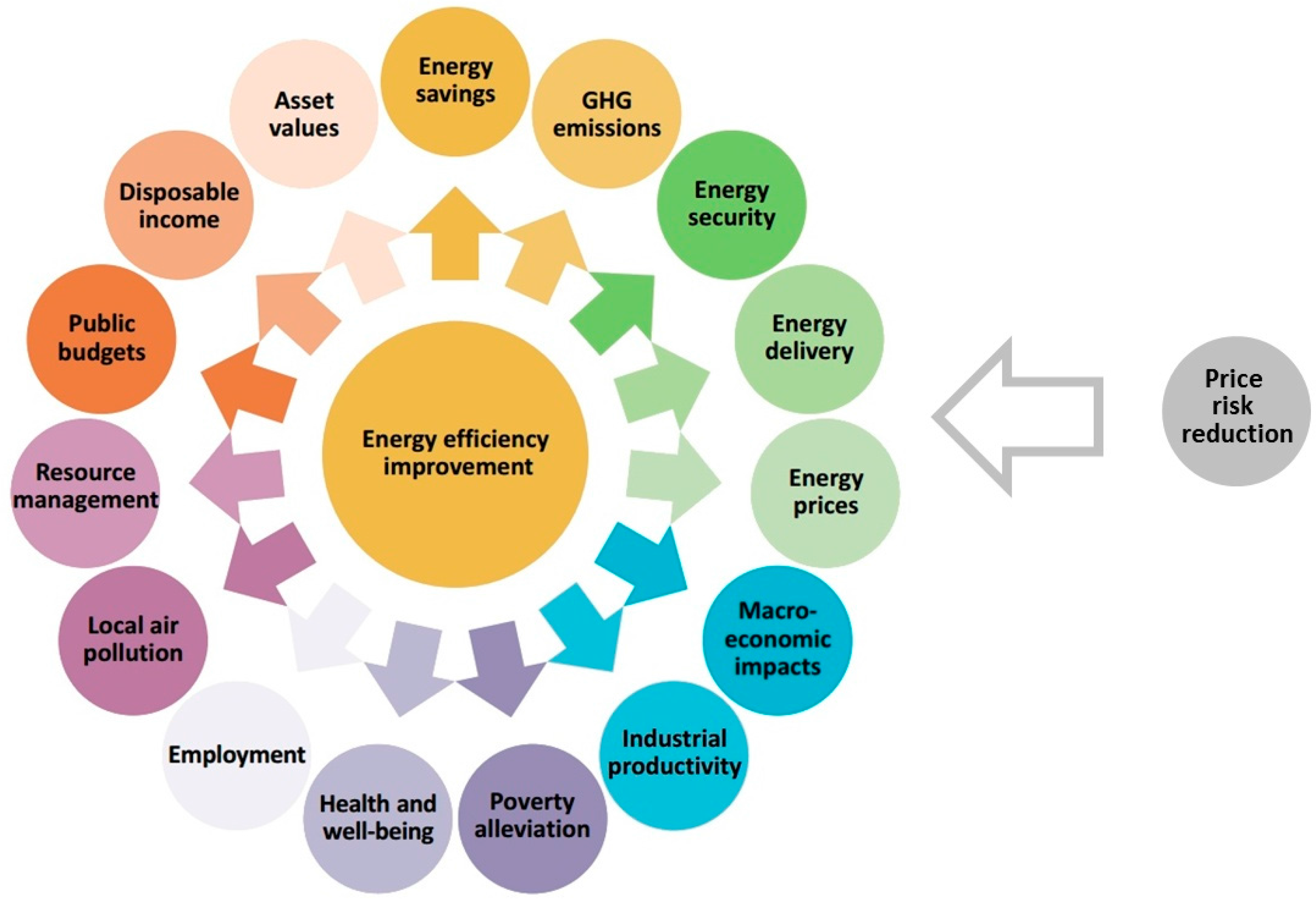
The IEA [14] and the US Environmental Protection Agency [15] are among the organizations that have recently recognized the importance of multiple benefits by producing major studies on the topic. IEA concluded that many of the multiple benefits have not been systematically assessed, in part because of the lack of proper methodologies to do so. Price risk reduction can be seen as one more area where a value to consumers can be recognized but not yet quantified, as is exemplified by Figure 1. This listing of benefits also shows that there are many different reasons why consumers may want to reduce energy consumption and cost savings and price risk reduction are but one of many. In this paper we concentrate on price risk reduction as other benefits have been extensively studied elsewhere in the literature (see e.g., [14,16]).
A consumer has interest in reducing her exposure to price risks in the market [17]. If investments in energy efficiency improvements in buildings are seen from the point of view of a consumer facing price risks from the energy market, then such investments can in part be seen to decrease uncertainty in future energy costs [18]. To state this differently, an energy-efficient building can be seen as protecting the consumer against rising energy costs insofar as energy consumption has been reduced and the consumer avoids paying the rising cost for the avoided share of energy consumption. Naturally this does nothing to remove any of the other types of risk that are inherently included in any construction investment, for instance, those relating to the interest for the capital or the risk that the investment fails to achieve its goals. Nevertheless, a reduction in the consumer’s price risk is an added and commonly overlooked benefit typical to energy-efficiency improvements specifically.
People who buy energy from the markets face the risk of rising energy prices. The standard approach to risky outcomes in economics is the von Neumann–Morgenstern utility function (see e.g., [19]). Utility, as it is meant here, can be defined as individual welfare or happiness or, functionally, as a summary of what guides individual choice [20]. The idea is that there are multiple possible outcomes xi, and for each xi there is a value v(xi) that the consumer assigns to them. The sum of all the values v weighted by their likelihood is the value the consumer assigns to the risky undertaking. Let the probability of each xi be πi. Then the von Neumann–Morgenstern function for economic utility u can be stated as follows:
If energy prices do indeed continue to rise, the payback periods for energy efficiency investments are shortened. After payback, the consumer who invested in an energy-efficient building would be accumulating a net profit that would be higher the higher the energy prices. The total cost for heating depending on the initial investment and energy prices can be treated as xi in Equation (1) and their respective likelihoods as πi.
The value function v of a typical consumer, shown in Figure 2, is thought to have a concave shape whereby higher levels of consumption provide a diminishing marginal utility. Such consumers will exhibit preference to average outcomes compared to random outcomes. This can be clarified with an example.
If the outcomes xa and xb in Figure 2 have a 50% likelihood each and they give the utilities va and vb respectively, then the consumer faces an expected value of utility of vev which is the average of va and vb. If, however, the consumer can instead choose the average outcome xav with a likelihood of 100%, then the consumer would receive the utility vav. Since this holds higher utility than vev, it is preferable compared to the random outcome.
Consumers with such preferences are called risk-averse. This means that the ability to lower the risk holds value to them. Thus, the fact that an energy-efficient building acts as an insurance against shifts in energy prices provides a premium to risk-averse consumers that does not show in simple investment calculations that concentrate on direct cost savings alone. To include this value of price risk reduction, a wider scope is needed in investment appraisal and a well-founded method to study the said value.
1.2. Review of Price Risk Valuation Methods
In financial economics, price risk or market risk is understood as the risk of financial losses caused by movements in market prices [21]. The standard approach to price risk management in the energy markets is through the derivatives market where futures and options allow energy buyers and sellers to protect themselves from adverse price fluctuations [22]. The market also allows defining a price for risk reduction by other means, as one has the alternative approach of insuring oneself against price risk using financial products. Any other approach, say an investment to energy efficiency, to reducing price risk makes economic sense only if it costs the same or less than an equivalent financial product in the derivatives market.
The standard approach to derivatives pricing in modern financial theory is the Black–Scholes model. The model is based on the assumption that the prices of traded assets follow a Brownian motion with constant drift and volatility [23]. In the context of finance, Brownian motion also called Wiener process refers to a random walk or succession of random steps that a financial variable, such as energy price, takes. Volatility refers to the rate at which the said financial variable moves up or down over time while drift refers to the change of the average value of the variable over time [20]. The applications of the Black–Scholes methodology in energy markets concentrate on options trading where the greatest financial interests are at stake [22].
Brennan and Schwartz [24] approach the problem of valuing uncertain cash flows of an investment project by trying to find a self-financing portfolio of traded securities whose cash flows replicate those which are to be valued. This approach is unsuitable for our case because its output is heavily dependent on market movements and does not produce a stable, simple and practical way of evaluating the value of the investment.
Woo et al. [25] offer a practical approach from a seller’s perspective where the seller’s risk premium is calculated by asking the following question: “What is the size of the per MWh risk premium that would allow a positive profit over some pre-determined time period with probability P?” While this is a very practical approach from a company’s perspective, it does not give any concrete estimate for the value of price risk reduction and hence cannot be used here.
Deng and Oren [26] suggest that due to the unique physical and operational characteristics of electricity production and transmission processes, classical derivative pricing methods based on geometric Brownian motion, such as the one used in this paper, may not work very well. Instead, they have suggested two alternative approaches. The “fundamental approach” relies on simulation of system and market operation to arrive at market prices, while the “technical approach” attempts to model directly the stochastic behavior of market prices from historical data and statistical analysis. Nevertheless, as our goal here is to present how such a calculation could be done in principle, we have chosen to use the most common method in financial industry utilizing geometric Brownian motion suggested by Black. The methods discussed by Deng and Oren [26] may offer a more well-founded approach in the case of electricity and, thus, offer a clear avenue for further study.
2. Methods
2.1. Calculating the Value of Price Risk Reduction
In this paper a variation of the Black–Scholes model is used to calculate the value of price risk reduction. This approach is selected because, for the purposes of this study, an approach that can be used to evaluate the price of price risk reduction in the electricity spot market is needed. It is postulated that with the emergence of market-priced spot electricity markets in the Nordic countries since the 1990s, it is possible to find the necessary data to employ the Black–Scholes methodology to produce useful results. Calculation examples are presented to show practical applications of the approach presented in this paper.
The problem is approached by considering a hypothetical financial instrument that a consumer would purchase to insure herself against unexpected price hikes. A rational consumer is prepared for a certain amount of growth in energy prices. If, however, the energy price rises more than expected, it might be very undesirable for the consumer. The consumer could, at least in theory, prepare for the unexpected rise by buying a cap contract on energy prices which would provide compensation for the unexpected rise. A cap contract bought from the financial markets means that the consumer is guaranteed never having to pay net prices over the agreed cap level. If market prices of energy are higher for a period of time, the consumer only pays a price equal to the cap, the rest being covered by the seller of the cap contract. This can be seen as an insurance policy against energy prices higher than the cap.
The value of a cap contract for the amount of saved energy consumption by an efficiency investment is the value of price risk reduction for the consumer. This is the theoretical fair economic value of the price risk reduction, meaning that in well-functioning financial markets it represents the price of buying capped price security for the same amount of energy consumption that the said energy efficiency investment has allowed to avoid altogether. However, such a cap contract should be viewed as hypothetical, as the practical options for consumers to protect themselves against unexpectedly high energy price rises depend on the market availability of such financial products.
To calculate the value of price risk reduction we use the Black [27] model—also called the Black–Scholes model—for pricing of commodity contracts, which is the standard approach used in the financial industry [28]. To be able to use the Black–Scholes model, a number of assumptions are made that are explained here. The underlying asset is the Spot price for Nord Pool (Nordic electricity exchange) energy price and historical data allows the calculation of volatility in the market. Risk-free interest rate is taken from Euribor yield curve. The expected future prices are estimated based on reasonable energy price inflation expectation, 2.5% for the examples presented here. The average electricity price inflation for single-family homes has been 3.3% annually since the liberalization of the Finnish electricity market in 1995, but in recent years the pace of inflation has been slowing down leading to 2.5% being used as a reasonable estimate [29]. The strike price for the cap contract, meaning the price at the level of the cap, depends on the consumer’s personal preference of tolerable energy pricing. For the calculation example we use 40% higher than expected as the tolerance level.
As any economic model, the Black–Scholes model is based on certain simplifications compared to real markets. These assumptions may not apply exactly for energy prices, but are nevertheless market practice and selected as a practical approach for the purposes of this paper [30]. The limitations of the Black–Scholes model mean that the results represent a theoretical fair economic value, meaning that while the results of the model are subject to inherent uncertainties, they are at the same time the standard approach in the market for valuating risky investments, and thus the valuation that both an informed seller and buyer would use in the absence of better information.
The Black–Scholes model assumes there are no taxes, margins or transaction costs. Moreover, the Black–Scholes model assumes that the volatility is constant and that the underlying asset price follows a lognormal distribution. This assumption can be used for the calculation of the theoretical fair economic value, but should be borne in mind when interpreting the results as real markets of course entail such costs. With these caveats in mind, the cap price can be stated as follows:
Here C is the price of the cap contract, meaning how much a customer would pay for the hypothetical price cap protection described above, t is the start time of the said cap contract (years from present), T is the end time of the cap contract, N is the energy consumption between t and T measured in kWh, P(0, T) is the value of a T maturity zero-coupon bond at present time, meaning the value of a bond that does not accrue interest but rather is sold at lower market price than its face value, F is the expected price of electricity at time T, K is the maximal tolerated price of electricity by the consumer at time T, meaning the cap value specified in the cap contract discussed above, N(x) is the cumulative normal distribution function and δ is the annualized electricity price volatility.
To calculate P(0, T), we use the current Euribor yield curve. To calculate δ, we use the historical electricity market prices for Finland [31]. To make the volatility figure realistic for our purposes, we have used average daily prices of working days and calculated the annualized volatility by multiplying the standard deviation of daily logarithmic returns, meaning logarithm of the quotient of the average prices of two consecutive working days, where Monday is considered as the next day after Friday, with the square root of yearly working days. For the years 2007–2012, this results in a volatility value of 2.0.
2.2. Electricity Price
As volatility is central to our reasoning, the consumer price used for the electricity consumed is based on daily prices in Nord Pool rather than on long-term fixed-price contracts. Even though the latter contract type is more commonplace, consumers in Finland do have the possibility to buy exchange-priced electricity through a number of power companies. In the case of the fixed-price contract, the energy company carries the price risk and it charges the customer a premium in return. However, as the energy company cannot affect the level of energy efficiency of the end user, at least not directly, this method is not applicable to it. Thus, a consumer with a market-priced contract is selected for applying the method.
The price data used in the calculations, summarized in Table 1, spans five years from 2007 to 2012 [31]. The consumer price is composed from the average daily spot price in Nord Pool for Finland, the average electricity tax, average value-added tax, typical power company’s price marginal and average transmission fee.
2.3. Case Buildings and Energy Consumption
The case buildings are variations on a typical Finnish single-family house, which is assumed to be electrically heated with direct electric radiators. This mode of heating remains the most common one in newly constructed single-family houses in Finland [34]. The buildings are assumed to have four dwellers, a typical size for a Finnish family, and to have a net area of 147 m² which is likely to be very close to the current average for new buildings. Sizes of new houses have been growing and were reported to be on average 144 m² in 2010 [35]. The buildings’ energetic properties were assumed to follow the 2010 government building regulations [36] and they are assumed to be located in southern Finland.
The different case buildings are as follows:
- Business as usual (BAU), with direct electric radiators as the only source of heat;
- BAU + fireplace, with a fireplace supplementing the radiators;
- BAU + heat pump, with an air source heat pump supplementing the radiators; and
- BAU + solar collectors, with roof-mounted solar heat collectors supplementing the radiators.
The building energy and financial calculations were done with the heating energy calculation tool of Motiva [37]. The calculation tool estimates that such a building would consume 4000 kWh/a for domestic water heating and 12,387 kWh/a for space heating, totaling 16,387 kWh/a. The heat pump is of air-to-air heat pump meaning that it uses as a heat source the outside air and heats directly the indoor air without circulation. It supplements the direct electric radiators in the BAU case. In the tool, the solar collectors have been sized so that they produce about 50% of domestic hot water and 30% of space heating over the year, which is roughly the optimum sizing for Finnish conditions. The sizing of the supplementary heat sources in the Motiva tool are based on Motiva corporation’s experiences from past energy efficiency projects and a study of 250 Finnish electrically heated single-family homes with implemented energy efficiency measures [2].
More details about the various heating systems are given in Table 2. Investment costs as well as energy consumption figures are those given as typical in the Motiva tool. In addition to electricity costs, the firewood is estimated to cost 200 €/a. No other running costs are assumed during the 20-year calculation period or, stated differently, it can be assumed that other running costs of the different alternatives are of similar scale and thus do not affect the calculations. In all the cases, the total delivered energy stays the same but the extra investments done in cases other than BAU allow a reduction in the amount of purchased electricity and thus, as the argument goes, also a reduction in the price risk the consumer faces in the electricity markets.
Table 3 shows the costs of the different cases in an annualized form. Investment costs have been annualized using an interest rate of 3%, which is typical for a Finnish housing loan [38]. Project lifespan used for financing calculations is set at 20 years. Variable costs are in this case cost of electricity purchasing to the consumer, consisting of the electricity spot price, electricity tax, VAT, power company’s price marginal and transmission costs.
3. Results
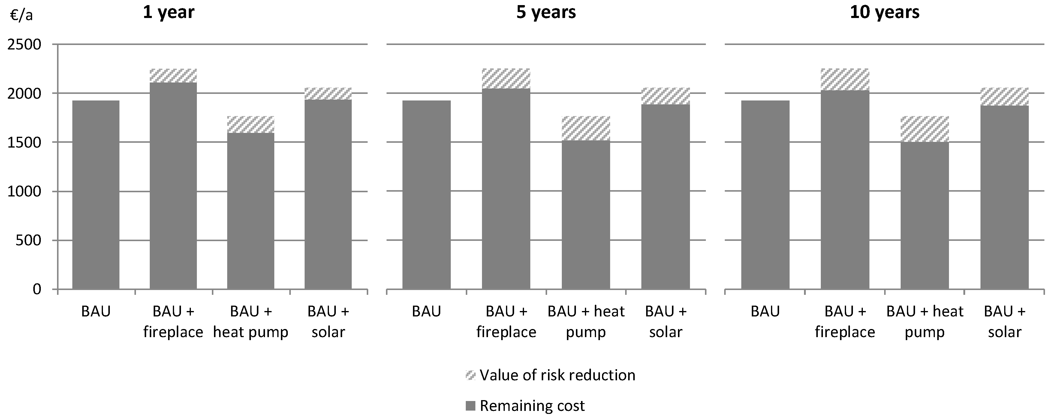
Value of price risk reduction to the consumer has been calculated in the case buildings listed in chapter 2.3. The results of the price risk reduction calculation are shown in Table 4 and in Figure 3. Total annualized cost of the project, excluding the value of risk reduction, has been carried from Table 3. The value of price risk reduction, presented as a negative figure, is subtracted from the total cost to produce remaining cost for each timespan. Three different timespans, extending 1 year, 5 years and 10 years to the future, are shown as the amount of price risk and thus the value of risk reduction is higher over longer periods of time according to the Black–Scholes model. The results in Table 4 show that the value of price risk reduction for the various investment alternatives appears to be around 10% of the total annualized costs: 6% at least and 15% at most.
4. Conclusions
This paper presents a method for calculating the value of price risk reduction to a consumer that can be achieved with investments in energy efficiency. It is based on the Black–Scholes model of pricing. Calculation examples are given for a case building with three investment alternatives for conserving purchased energy and thus reducing the risk of adverse effects from future price changes.
The calculation example demonstrates that a working valuation model for quantifying the value of price risk reduction is possible to construct given the information available from the markets. From the results concerning the case building, it can be seen that the value of the risk reduction provided by an energy efficiency improvement can be calculated using the proposed method. Using the method presented here, a similar calculation can be reproduced for any case where the necessary parameters for the Black–Scholes model can be found. In practice this means an energy efficiency investment that reduces energy consumption for an energy carrier that has the market price data available necessary for defining the implied volatility. This is also the main limitation of this approach because many energy forms do not have such markets where they are traded freely. In this case, electricity price history in the Nordic electricity market provided the needed data.
Based on the examples calculated in this paper, the value of price risk reduction is estimated to be around 10% of the total annualized costs for typical energy efficiency investments in typical single-family homes in Finland. As Figure 3 demonstrates, this can be interpreted as making the investment more attractive when the value of price risk reduction is included in the total. Because of discounting, reduction of risks further away in the future appears more valuable and thus expanding the timespan of the calculation from one year to five or ten increases the value of price risk reduction. Therefore, the exact value of price risk reduction is dependent on how long a view the consumer takes on her investment.
While the examples presented in this paper deal with heating electricity, the same principle is applicable to other efficiency improvements in electricity use or other forms of energy. After all, improving levels of insulation in new buildings means that heating consumption tends to decrease while electricity consumption for appliances may continue to increase. Additionally, it should be noted that the choice of examples was partly done for simplicity. While protecting oneself against energy price increases is also relevant for homeowners, perhaps in reality the likeliest early adopters of this type of approach to managing price risk are corporations or institutions that own large amounts of real estate and thus have significant exposure to fluctuations in the energy market.
In the case studied, the value of price risk reduction is large enough to have an effect on the decision whether to invest. Especially in cases where investments appear marginally profitable, even a benefit of about 10% can have a pivotal role. Moreover, there are circumstances in which the value of price risk reduction can be higher, such as more volatile markets or investments with smart control of the energy consumption to compensate for fluctuating energy prices.
There is also a methodological issue that means that this value estimate can be somewhat conservative: the Black–Scholes model may underestimate the value of price risk reduction in energy markets because it is based on the use of interest rates from the financial markets as reference, and energy commodities often possess more heavy-tailed price distributions in comparison. Overall, the study shows that price risk reduction is a quantifiable benefit of energy efficiency investments in buildings that is large enough to be non-trivial.
As was discussed in the introduction, it is recognized that the Black–Scholes model may harbor other shortcomings for analyses dealing with electricity prices. Thus, other potential methodological approaches should be further explored, including the possible tweaking of the Black–Scholes equation or the use of the Deng and Oren [26] approach. To have a fuller accounting of the benefits of energy efficiency investments, the issue of price risk reduction merits further research.
Acknowledgments
This research has been supported by the project Assessing the intangibles: the socioeconomic benefits of improving energy efficiency (IN-BEE) funded by the Intelligent Energy Europe program of the European Commission.
Author Contributions
Pekka Tuominen has been mainly responsible for the parts dealing with energy efficiency while Tuomas Seppänen has been mainly responsible for the financial parts in this study.
Conflicts of Interest
The authors declare no conflict of interest.
References
- Al-Sunaidy, A.; Green, R. Electricity deregulation in OECD countries. Energy 2006, 31, 769–787. [Google Scholar] [CrossRef]
- Kokkonen, A. Sähkölämmityksen Tehostamisohjelma Elvari Loppuraportti; Motiva: Helsinki, Finland, 2015. [Google Scholar]
- Laustsen, J. Energy Efficiency Requirements in Building Codes, Energy Efficiency Policies for New Buildings; International Energy Agency: Paris, France, 2008. [Google Scholar]
- Gillingham, K.; Newell, R.G.; Palmer, K. Energy Efficiency Economics and Policy. Annu. Rev. Resour. Econ. 2009, 1, 597–620. [Google Scholar] [CrossRef]
- Brown, M. Obstacles to Energy Efficiency. In Encyclopedia of Energy; Cleveland, C., Ed.; Elsevier: San Diego, CA, USA, 2004; pp. 465–475. [Google Scholar]
- Klemick, H.; Wolverton, A. Energy-efficiency gap. In Encyclopedia of Energy; Cleveland, C., Ed.; Elsevier: San Diego, CA, USA, 2004. [Google Scholar]
- Abadie, L.M.; Chamorro, J.M.; González-Eguino, M. Valuing uncertain cash flows from investments that enhance energy efficiency. J. Environ. Manag. 2013, 116, 113–124. [Google Scholar] [CrossRef] [PubMed]
- Jackson, J. Promoting energy efficiency investments with risk management decision tools. Energy Policy 2010, 38, 3865–3873. [Google Scholar] [CrossRef]
- Tuominen, P.; Reda, F.; Dawoud, W.; Elboshy, B.; Elshafei, G.; Negm, A. Economic appraisal of energy efficiency in buildings using cost-effectiveness assessment. Proced. Econ. Financ. 2015, 21, 422–430. [Google Scholar] [CrossRef]
- Vine, E.; Mills, E.; Chen, A. Energy-efficiency and renewable energy options for risk management and insurance loss reduction. Energy 2000, 25, 131–147. [Google Scholar] [CrossRef]
- Thompson, P. Evaluating energy efficiency investments: Accounting for risk in the discounting process. Energy Policy 1997, 25, 989–996. [Google Scholar] [CrossRef]
- Weinsziehr, T.; Skumatz, L. Evidence for Multiple Benefits or NEBs: Review on Progress and Gaps from the IEA Data and Measurement Subcommittee. In Proceedings of the International Energy Policy & Programme Evaluation Conference, Amsterdam, The Netherlands, 7–9 June 2016. [Google Scholar]
- Ürge-Vorsatz, D.; Novikova, A.; Sharmina, M. Counting good: Quantifying the co-benefits of improved efficiency in buildings. In Proceedings of the ECEEE 2009 Summer Study, Stockholm, Sweden, 1–6 June 2009. [Google Scholar]
- International Energy Agency. Capturing the Multiple Benefits of Energy Efficiency; International Energy Agency: Paris, France, 2014. [Google Scholar]
- U.S. Environmental Protection Agency. Assessing the Multiple Benefits of Clean Energy; U.S. Environmental Protection Agency: Washington, DC, USA, 2011.
- Tuominen, P.; Holopainen, R.; Eskola, L.; Jokisalo, J.; Airaksinen, M. Calculation method and tool for assessing energy consumption in the building stock. Build. Environ. 2014, 75, 153–160. [Google Scholar] [CrossRef]
- Conchar, M.; Zinkhan, G.; Peters, C.; Olavarrieta, S. An Integrated Framework for the Conceptualization of Consumers’ Perceived Risk. J. Acad. Mark. Sci. 2004, 32, 418–436. [Google Scholar] [CrossRef]
- Electricity Authority. Managing Electricity Price Risk; Electricity Authority: Wellington, New Zeeland, 2012. [Google Scholar]
- Mas-Colell, A.; Whinston, M.; Green, J. Microeconomic Theory; Oxford University Press: New York, NY, USA, 1995. [Google Scholar]
- Black, J.; Hashimzade, N.; Myles, G. A Dictionary of Economics; Oxford University Press: Oxford, UK, 2009. [Google Scholar]
- Bank for International Settlements. A Glossary of Terms Used in Payments and Settlement Systems; Bank for International Settlements: Basel, Switzerland, 2003. [Google Scholar]
- James, T. Energy Markets: Price Risk Management and Trading; John Wiley & Sons: Singapore, 2012. [Google Scholar]
- Profeta, C.; Roynette, B.; Yor, M. Option Prices as Probabilities: A New Look at Generalized Black-Scholes Formulae; Springer: Berlin, Germany, 2010. [Google Scholar]
- Brennan, M.; Schwartz, E. Evaluating natural resource investments. J. Bus. 1985, 2, 135–157. [Google Scholar] [CrossRef]
- Woo, C.-K.; Horowitz, I.; Hoang, K. Cross hedging and forward-contract pricing of electricity. Energy Econ. 2001, 23, 1–15. [Google Scholar] [CrossRef]
- Deng, S.; Oren, S. Electricity derivatives and risk management. Energy 2006, 31, 940–953. [Google Scholar] [CrossRef]
- Black, F. The pricing of commodity contracts. J. Financ. Econ. 1976, 3, 167–179. [Google Scholar] [CrossRef]
- Zvi, B.; Kane, A.; Marcus, A. Investments; McGraw-Hill/Irwin: New York, NY, USA, 2008. [Google Scholar]
- Statistics Finland. Energian hinnat. Available online: http://stat.fi/til/ehi/tau.html (accessed on 20 September 2017).
- Eydeland, A.; Wolyniec, K. Energy and Power Risk Management: New Developments in Modelling, Pricing and Hedging; John Wiley & Sons: Hoboken, NJ, USA, 2003. [Google Scholar]
- Nord Pool. Elspot Prices. Available online: http://www.nordpoolspot.com/Market-data1/Elspot/Area-Prices/ (accessed on 1 April 2014).
- Energy Authority. Sähkön hintatilastot. Available online: http://www.energiavirasto.fi/sahkon-hintatilastot (accessed on 12 May 2014).
- Energiapolar. Polar Spot Hinnat ja Ehdot. Available online: https://www.energiapolar.fi/loader.aspx?id=4f88ac11-60ba-4160-8d5a-9f86a1e2a168 (accessed on 12 May 2014).
- Vilhola, J.; Heljo, J. Lämmitystapojen kehitys 2002–2012; Tampere University of Technology: Tampere, Finland, 2012. [Google Scholar]
- Tiihonen, A. Asumisväljyys Lisääntyy Hitaasti; Statistics Finland: Helsinki, Finland, 2011. [Google Scholar]
- Ministry of the Environment. D3 Energy Management in Buildings, Regulations and Guidelines 2010; Ministry of the Environment: Helsinki, Finland, 2010.
- Motiva. Lämmitystapojen Vertailulaskuri. Available online: http://lammitysvertailu.eneuvonta.fi (accessed on 21 March 2014).
- Bank of Finland. Monetary Financial Institutions Annual Review 2013; Bank of Finland: Helsinki, Finland, 2014. [Google Scholar]
Figure 1.
The most prominent types of multiple benefits of energy efficiency improvements, as listed by the International Energy Agency (IEA) [14], are supplemented by the value of price risk reduction. This figure is adapted from a graphic by IEA [14].

Figure 2.
The utility function of a risk-averse consumer.
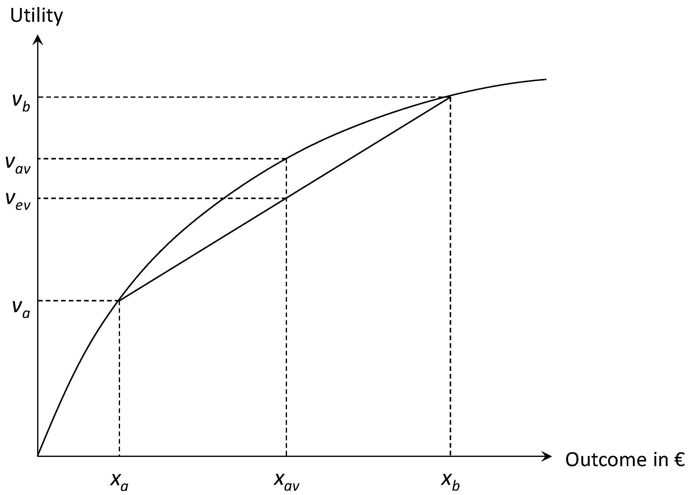
Figure 3.
The value of price risk reduction and remaining cost in each case for three different timespans used in the calculation.
Figure 3.
The value of price risk reduction and remaining cost in each case for three different timespans used in the calculation.

Table 1.
The average makeup of the electricity price for consumers during the period studied (2007–2012).
Table 1.
The average makeup of the electricity price for consumers during the period studied (2007–2012).
| Price Component | Amount (c/kWh) | Source |
|---|---|---|
| Electricity spot price | 4.34 | [31] |
| Electricity tax | 1.39 | [32] |
| Value-added tax | 0.97 | [31] |
| Power company price marginal | 0.25 | [33] |
| Transmission fee | 3.16 | [31] |
| Total consumer price | 10.11 | - |
Table 2.
Key figures concerning the heating systems in the different cases. BAU stands for Business as usual.
Table 2.
Key figures concerning the heating systems in the different cases. BAU stands for Business as usual.
| Indicator | BAU | BAU + Fireplace | BAU + Heat Pump | BAU + Solar |
|---|---|---|---|---|
| Investment cost (€) | 4000 | 9500 | 6000 | 10,000 |
| Electricity consumption (kWh/a) | 16,387 | 13,984 | 13,488 | 14,370 |
| Other heat sources (kWh/a) | 0 | 2403 | 2899 | 2017 |
Table 3.
Annualized costs (€/a) of the heating system in the different cases.
| Cost Type | BAU | BAU + Fireplace | BAU + Heat Pump | BAU + Solar |
|---|---|---|---|---|
| Variable cost | 1655 | 1612 | 1362 | 1451 |
| Capital cost | 269 | 639 | 403 | 605 |
| Total cost | 1924 | 2251 | 1765 | 2056 |
Table 4.
Accounting of annualized costs to the investor in the four cases over three different time periods. Total annualized cost (€/a) shows annualized cost of each type of heating system, value of risk reduction (€/a) shows the value of risk reduction in each case and time period as a negative cost, remaining cost (€/a) shows the total cost of the heating system after subtracting the value of price risk reduction and, finally, relative value (%) shows the relative value of price risk reduction compared to the total cost of the heating system in each case and for each time period.
| Time Period | Type of Cost or Value | BAU | BAU + Fireplace | BAU + Heat Pump | BAU + Solar |
|---|---|---|---|---|---|
| - | Total annualized cost | 1924 | 2251 | 1765 | 2056 |
| 1 year | Value of risk reduction | 0 | −140 | −168 | −117 |
| Remaining cost | 1924 | 2111 | 1597 | 1939 | |
| Relative value | 0% | 6% | 10% | 6% | |
| 5 years | Value of risk reduction | 0 | −204 | −247 | −172 |
| Remaining cost | 1924 | 2047 | 1518 | 1884 | |
| Relative value | 0% | 9% | 14% | 8% | |
| 10 years | Value of risk reduction | 0 | −218 | −263 | −183 |
| Remaining cost | 1924 | 2033 | 1502 | 1873 | |
| Relative value | 0% | 10% | 15% | 9% |
© 2017 by the authors. Licensee MDPI, Basel, Switzerland. This article is an open access article distributed under the terms and conditions of the Creative Commons Attribution (CC BY) license (http://creativecommons.org/licenses/by/4.0/).
Share and Cite
MDPI and ACS Style
Tuominen, P.; Seppänen, T. Estimating the Value of Price Risk Reduction in Energy Efficiency Investments in Buildings. Energies 2017, 10, 1545. https://doi.org/10.3390/en10101545
AMA Style
Tuominen P, Seppänen T. Estimating the Value of Price Risk Reduction in Energy Efficiency Investments in Buildings. Energies. 2017; 10(10):1545. https://doi.org/10.3390/en10101545
Chicago/Turabian StyleTuominen, Pekka, and Tuomas Seppänen. 2017. "Estimating the Value of Price Risk Reduction in Energy Efficiency Investments in Buildings" Energies 10, no. 10: 1545. https://doi.org/10.3390/en10101545
Note that from the first issue of 2016, this journal uses article numbers instead of page numbers. See further details here.