Dynamic Process Model Validation and Control of the Amine Plant at CO2 Technology Centre Mongstad


1
Department of Energy and Process Engineering, NTNU—Norwegian University of Science and Technology, NO-7491 Trondheim, Norway
2
CO2 Technology Center Mongstad, NO-5954 Mongstad, Norway
*
Author to whom correspondence should be addressed.
Energies 2017, 10(10), 1527; https://doi.org/10.3390/en10101527
Submission received: 24 August 2017
/
Revised: 21 September 2017
/
Accepted: 26 September 2017
/
Published: 1 October 2017
Abstract
:This paper presents a set of steady-state and transient data for dynamic process model validation of the chemical absorption process with monoethanolamine (MEA) for post-combustion CO2 capture of exhaust gas from a natural gas-fired power plant. The data selection includes a wide range of steady-state operating conditions and transient tests. A dynamic process model developed in the open physical modeling language Modelica is validated. The model is utilized to evaluate the open-loop transient performance at different loads of the plant, showing that pilot plant main process variables respond more slowly at lower operating loads of the plant, to step changes in main process inputs and disturbances. The performance of four decentralized control structures is evaluated, for fast load change transient events. Manipulation of reboiler duty to control CO2 capture ratio at the absorber’s inlet and rich solvent flow rate to control the stripper bottom solvent temperature showed the best performance.
1. Introduction
Carbon capture and storage (CCS) is a group of technologies that can significantly contribute to the reduction of anthropogenic CO2 emissions from thermal power generation and other carbon-intensive industries [1]. There are two commercial-scale coal-fired power plants with post-combustion CO2 capture (PCC) using amines being operated today, at Boundary Dam in Canada [2] and at Petra Nova project at the Parish Power Station in the US [3]. These projects prove the technical feasibility of the technology at commercial scale. Among the different options and technologies for CO2 capture in thermal power generation, post-combustion CO2 capture with chemical absorption is considered the more mature technology that can contribute to significantly reducing the carbon intensity (kgCO2/kWhel) of fossil-fueled thermal power plants. In future energy systems with a high penetration of renewable energy sources, the variability in demand and generation will introduce a change in the operating patterns of thermal power generation plants, which will have to change operating conditions [4,5,6]; there will also be a higher frequency of significant transient events including load changes, and start-up and shut-down events [7,8]. In this regard, Boot-Handford et al.’s carbon capture and storage update 2014 concludes that the financial case for CCS requires that it operates in a flexible manner and that load-following ability is extremely important to the long-term economics [9].
Among the different features of flexible operation of power plants with CCS, an important aspect is the transient behavior of the system when varying operating conditions. This means that efficient operation and emissions and the related operational costs during transient operation will gain importance. However, the operational experience from commercial-scale power plants with post combustion CO2 capture is scarce and the published transient pilot plant data from test campaigns is limited. Therefore, there is a need for the development of dynamic process models. Dynamic process models can contribute to developing the learning curve for flexible operation of PCC plants. These tools can assist in evaluating the feasibility of flexible operation strategies as well as design process configurations and operational strategies that can lead to the reduction of operational costs and increased revenue during power plant operation. The study of the transient performance with dynamic process models can contribute to identifying process bottlenecks and ease the process scale-up.
Dynamic process models allow the study of the open-loop transient performance of the plant [10], the evaluation of different process configurations and designs [11], the development and implementation of optimal control strategies [12,13,14,15,16,17,18,19,20], as well as the study of the plant behavior under different operational flexibility scenarios [21,22]. In addition, the power plant and the PCC unit can be treated as an integrated system and dynamic process models can be utilized to analyze the response of the capture unit to changes that occur upstream in the power plant [12,15,19,23,24,25]. Furthermore, the operational flexibility of the PCC plant can be improved with plant design or using control strategies [26,27,28,29]. The core purpose of dynamic process models is to capture the time-dependent behavior of the process under transient conditions. However, the validation of dynamic process models with experiments and pilot plant data is necessary in order to assess the reliability of simulation results.
Kvamsdal et al. [30] developed a dynamic process model of a CO2 absorber column and used steady-state data from a pilot plant to validate liquid temperature profiles, capture ratio % and rich loading. That work highlighted the necessity of building up a dynamic process model of the integrated system (including stripper, lean/rich heat exchanger, mixing tank and main process equipment), to understand the complexities of dynamic operation of the plant. Gaspar and Cormos [31] developed a dynamic process model of the absorber/desorber process and validated with steady-state plant data. Several publications are available, in which the models were validated only with steady-state pilot plant data [11,32,33,34,35]. Biliyok et al. [36] presented a dynamic model validation study where transient data was driven by decrease in solvent flow rate to the absorber, fluctuating concentration of CO2 at absorber inlet and a varying absorber’s feed flue gas stream temperature to the absorber. A dynamic process model developed in Modelica language was validated with transient data from the Esbjerg pilot plant by Åkesson et al. [37]. That data consisted of the transient performance after one step-change in flue gas mass flow rate. An extensive review work by Bui et al. [38] concluded that research efforts are required on producing transient pilot plant data.
More recent works have included validation of dynamic process models with transient plant data from pilot plants. A K-Spice model by Flø et al. was validated with pilot plant data from the Brindisi pilot plant [39]. Flø et al. [40] validated a dynamic process model of CO2 absorption process, developed in Matlab, with steady-state and transient pilot plant data from the Gløshaugen (Norwegian University of Science and Technology (NTNU)/SINTEF) pilot plant. Van de Haar et al. [41] conducted dynamic process model validation of a dynamic process model in Modelica with transient data from a pilot plant located at the site of the coal-fired Maasvlakte power plant in the Netherlands. Gaspar et al. [42] conducted model validation with transient data from two step changes in flue gas volumetric flow rate from the Esbjerg pilot plant. Other works include the validation of equilibrium-based models such as that of Dutta et al. [43]; or the work by Chinen et al. [44] which conducted dynamic process model validation of a process model in Aspen Plus® with transient plant data from the National Carbon Capture Center (NCCC) in the US. Manaf et al. [45] developed a data-driven black box mathematical model, based on transient pilot plant data, by means of system identification. In addition, dynamic process models have been developed to study the transient behavior of the chemical absorption CO2 capture process using piperazine (PZ) as chemical solvent [19,20]. It should be noted that the majority of work has been conducted for typical flue gas compositions from coal-based power plants with CO2 concentration around 12 vol % [38].
From the literature review it can be concluded that dynamic process model validation is a challenging process due to:
- The scarce availability of transient or dynamic pilot plant data.
- Most available data is found from small-scale pilot plants. That has implications for the reliability of simulation results when applying dynamic process models to scaled-up applications.
- The works involving transient data generally include the response of the plant to disturbances in a few process variables.
- Most of the validation work was done for flue gas with a typical CO2 content from coal-based power plants.
Flexible operation of PCC plants has been studied with pilot plant test facilities in test campaigns. Faber et al. [46] conducted open-loop step change responses at the Esbjerg pilot plant; this type of analysis helps in understanding the transient performance of the process. They concluded that the overall system acts as a buffer to perturbations at the plant inlet and that the coupled operation of the absorber/desorber unit led to fluctuations in the system when all parameters—flue gas and solvent mass flow rates and reboiler duty—are changed simultaneously. Bui et al. [47] presented a flexible operation campaign conducted at the Commonwealth Scientific and Industrial Research Organization (CSIRO)’s PCC pilot plant in Australian Gas Light Company (AGL) Loy Yang, a brown-coal-fired power station in Australia. The generated transient data included step changes in flue gas flow rate, solvent flow rate and steam pressure. The purpose of the study was to generate a set of data for validation of dynamic process models, and to gain insight into process behavior under varying operating conditions. A different approach was taken by Tait et al. [48] who conducted experiments that simulated flexible operation scenarios on a pilot plant to treat synthetic flue gas with a CO2 concentration of 4.3 vol%, typical of a natural gas combined cycle (NGCC) plant. Tests for transient operation have been conducted at the amine plant at CO2 Technology Center Mongstad (TCM DA). De Koeijer et al. presented two cases: a first case with controlled stop-restart of the plant, driven by a controlled stop of flue gas and steam sent to the PCC plant; and a second case with sudden stop of the blower upstream of the absorber [49]. Nevertheless, a limited amount of transient testing can be conducted during test campaigns. A thoroughly validated dynamic process model can help to study the transient performance, controllability, and flexible operation of the plant and process dynamics via dynamic process simulation.
In this work, a suitable set of steady-state and transient plant data, collected from a MEA campaign at CO2 Technology Center Mongstad, is selected for dynamic process model validation purposes. The plant was operated with flue gas from a natural gas fueled combined heat and power plant. The selected data is utilized to validate a dynamic process model of the amine-based CO2 absorption-desorption process at TCM DA. Then, the validated model is employed to carry out two case studies on the process dynamics of the TCM DA amine plant. In the first case study, the open-loop transient response of the pilot plant at different operating loads of the plant is analyzed. In the second case study, the performance of four decentralized control structures of TCM DA amine pilot plant is evaluated for fast disturbances in flue gas volumetric flow rate.
2. Materials and Methods
2.1. Plant Description
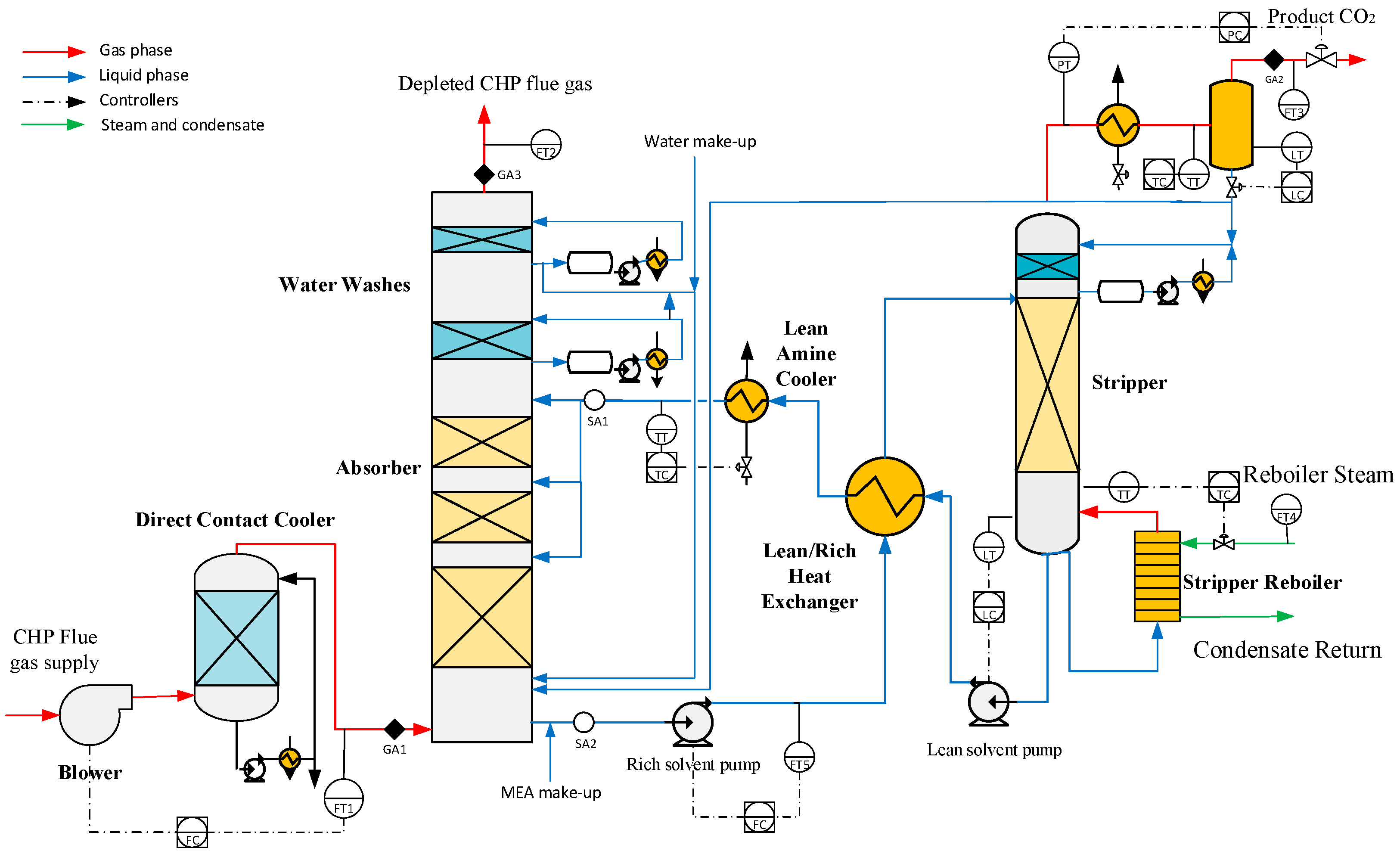
CO2 Technology Center Mongstad test site has a pilot-scale amine-based chemical absorption process plant. The amine plant can be configured to treat flue gas from a catalytic cracker from the Mongstad refinery, with CO2 content of around 13–14 vol%, typically found in flue gas from coal-fired power plants, and also to treat exhaust gas coming from a combined cycle gas turbine combined heat and power plant (CHP), with CO2 content of around 3.5 vol%. A fraction of the product CO2 mass flow rate can be re-circulated back upstream of the direct contact cooler (DCC) to increase the CO2 content, so CO2 concentrations of between 3.5 and 13–14 vol% could be fed to the plant to simulate the effects of exhaust gas recirculation [50]. Table 1 presents data of the main process equipment of TCM DA amine plant when configured to treat CHP flue gas, which has a total flue gas capacity of 60,000 Sm3/h and can capture around 80 ton CO2/day. Figure 1 shows a simplified process flow sheet of the amine plant at TCM DA when configured for CHP gas. A slipstream of exhaust gas is extracted from the CHP plant placed next to the TCM DA facility, and it consists of about 3% of the total exhaust gas. An induced draft blower is utilized to blow the flue gas flow. It has variable speed drives that allow the flue gas volumetric flow rate fed to the absorber column to be manipulated. Upstream the absorber column, a direct contact cooler cools down and saturates the flue gas with water, by means of a counter-current flow stream of water.
A chemical absorption process occurs in the absorber column, where the chemical solvent, flowing from top to bottom, meets the flue gas flowing in counter-current. The absorber column consists of a rectangular polypropylene-lined concrete column with a height of 62 m and a cross-section of 2 × 3.55 m. The absorber-packed sections consisting of Flexipac 2X (Koch-Glitsch Italia, Vimercate, Italy) structured stainless-steel packing are distributed from bottom to top in three sections of 12 m, 6 m and 6 m. Two water-wash systems are installed in the top of the absorption column, consisting of two sections of Flexipac 2Y HC (Koch-Glitsch Italia, Vimercate, Italy) structured stainless-steel packing. The water-wash sections limit emissions and are used to keep the water balance of the plant. The upper water-wash sections can be operated as acid wash [51]. In addition, the plant can be configured to use different packing heights in the absorber column resulting in 12, 18 or 24 m. This can be implemented at TCM plant by introducing all the lean solvent flow at 12 m of absorber packing, 18 m of absorber packing (12 + 6) m or 24 m of absorber packing (12 + 6 + 6) m.
A 10.4 MW plate and frame heat exchanger is present at the plant where the cold rich amine solution coming from the absorber sump cools down the hot lean amine solution coming from the stripper. In addition, a 5.2 MW lean amine cooler is utilized to set the temperature of the lean solvent conducted to the top of the absorber packing sections, by using a stream of cooling water. The rich solvent is pumped to the top of the stripper column, where it meets the stripping vapors generated in the reboiler. The CHP stripper with overhead condenser system consists of an 8 m column of Koch Glitsch Flexipac 2X structured stainless-steel packing of 1.3-m-diameter, and a water-wash system with Koch Glitsch Flexipac 2Y HC structured stainless-steel packing of 1.6 m of height. The stripper reboiler consists of a 3.4 MW thermosiphon steam-driven system that supplies the heat required for the desorption process. The steam supplied to the reboiler comes from the refinery situated next to the TCM DA facility. Details on the steam supply system can be found in Faramarzi et al. [51].
2.2. Pilot Plant Configuration and Instrumentation
The TCM DA amine plant can be utilized to test various chemical solvents. In this work, the tests were conducted with 30 wt. % aqueous monoethanolamine (MEA). During the tests conducted in the test campaign, the responses and performance of the pilot plant were logged and extracted every 30 s. Gas composition was logged with gas analyzers at the inlet of the absorber, outlet of the absorber, and the product CO2. A gas chromatograph (GC) installed at TCM DA plant can measure concentrations of CO2, N2, H2O and O2 at the three locations in a nearly simultaneous manner, which is a desired feature for transient tests; refer to GA1, GA2 and GA3 in Figure 1. Details on gas analyzers and instrumentation at TCM DA plant can be found in [51].
Gas phase flow rates were measured at the plant during the tests. The flue gas volumetric flow rate fed to the absorber is measured with an ultra-sonic flow meter (FT1). As discussed by Faramarzi et al. in [51], the depleted flue gas flow meter (FT2) had a higher degree of variability than FT1, and some transients were observed on the FT2 measurement that were not explained by changes in process parameters at the plant. Therefore the depleted flue gas flow rate was calculated in the test campaign by considering that all O2 and N2 fed to the absorber goes out of the plant with the depleted flue gas. The cooled product CO2 discharge flow (FT3) was measured with a vortex flow meter. Other flow rates measured at the plant include the steam fed to the reboiler, the lean amine flow rate at the absorber inlet and the rich amine flow rate at the absorber outlet. For flue gas flow meters, the standard conditions are 15 °C and 101.3 kPa [51].
Pressures and pressure drops at different components of the plant were logged. In addition, main process temperatures were logged. For process model validation, it is common to assess the model prediction of the absorber and stripper temperature profiles. Within the absorber and stripper columns of TCM DA’s amine plant there are four temperature sensors distributed in the radial plane per meter of packing in the axial direction. Thus, there are 96 temperature sensors within packed segments of absorber column and 28 temperature sensors within the packed segment in the stripper column. These measurements allow the creation of clear temperature profiles of the absorber and stripper columns in the axial direction (at each column height, the resulting temperature value is the average of the four measurements distributed in the radial plane).
Online solvent analysis measurements (SA) were taken at the inlet (SA1) and outlet of the absorber (SA2); refer to Figure 1. The measurements include pH, density and conductivity. In addition, solvent samples were regularly taken manually and analyzed onsite. These analyses allow MEA concentration and CO2 loadings to be calculated at the sampling points on a periodic basis. The actual reboiler duty was estimated as suggested in Thimsen et al. [52]. Equation (1) shows the calculation of the actual reboiler duty, where is the logged measurement data of steam mass flow rate (refer to FT4 in Figure 1), is the condensate temperature, is the superheated steam inlet temperature, is the steam pressure at inlet, and is the condensate pressure. Enthalpy was calculated with the use of accurate steam tables, with the condensate at the reboiler outlet assumed to be saturated liquid at or . The specific reboiler duty (SRD) in kJ/kgCO2 is calculated as in Equation (2), where Fprod is the CO2 rich product mass flow rate; refer to FT3 in Figure 1.
During the tests presented in this work, the averaged total inventory of aqueous MEA was around 38.2 m3. Averaged values of liquid hold-ups and its distribution at different components of the plant during the steady-state tests included in this work are presented in Table 2. Detailed data on solvent inventory distribution throughout the plant is of importance in order to obtain suitable dynamic process simulation results. The regulatory control layer of the plant was active during the tests conducted in the MEA campaign. The main control loops of the regulatory control layer are presented in Figure 1. Note that the actual regulatory control layer of the amine plant at TCM DA is more complex and includes more control loops for auxiliary equipment, stable and safe operation of the plant, and start-up and shut-down sequences. The control loops included here are those the authors found relevant for the purposes of dynamic process modeling and simulation of this plant during online operation, and considering the time scales of interest for process operation.
2.3. Dynamic Process Model
Dynamic process modeling was carried out by means of the physical modeling language Modelica [53]. Modelica allows development of systems of differential and algebraic equations that represent the physical phenomena occurring in the different components of the system. The process models of the equipment typically found in a chemical absorption plant were obtained from a Modelica library called Gas Liquid Contactors (Modelon AB, Lund, Sweden) [54], and the commercial tool Dymola (Dassault Systèmes, Vélizy-Villacoublay, France) [55] was utilized to develop the models and carry out the simulations. The component models include absorber and stripper columns, sumps, lean and rich heat exchanger, stripper reboiler, overhead condenser, condensers, pipe models, pumps, valves, measurements and controllers. The dynamic process model of the amine plant at TCM DA presented in Figure 1 was developed by parameterizing, modifying and connecting the different models. For this purpose, the main process equipment, size, geometry and materials were considered; refer to Table 1. A key aspect for obtaining suitable dynamic simulation results is the consideration of the distribution of solvent inventory at the different equipment of the plant. Therefore, solvent inventory distribution was implemented in the dynamic process model; refer to Table 2. Finally, the equivalent regulatory control layer of the plant was applied in the dynamic process model; discussed later in Section 5.2. The models contained in the library have been presented elsewhere [56,57]; therefore only an overview of the models is presented in the following. Numerical integration of the resulting system of differential and algebraic equations was carried out in Dymola with the differential algebraic system solver (DASSL) implemented in Dymola [55]. The main assumptions applied are [56]:
- All chemical reactions occur in the liquid phase and are assumed to be in equilibrium.
- The flue gas into the absorber contains only CO2, O2, H2O and N2.
- MEA is non-volatile and not present in the gas phase.
- The total amount of liquid in the column is defined as the packing hold-up and the sump liquid hold-up.
- The reboiler is modeled as an equilibrium flash stage.
- The liquid in the column sumps and other large volumes are assumed to be ideally mixed.
- Mass and heat transfer between liquid and gas phase is restricted to packed section.
- Negligible temperature difference between the liquid bulk and interface to gas phase.
- No storage of mass and energy in the gas phase.
- All liquid from the packing bottom in the stripper is fed to the reboiler with a constant liquid level.
- Constant target packing hold-up.
The models of the absorber and stripper columns are developed based on the two-film theory; therefore, at the gas and liquid interface thermodynamic equilibrium is assumed. Interface mass transfer phenomena is modeled in packed sections with a rate-based approach with enhancement factor E [30], which takes into account the enhanced mass transfer due to chemical reactions; refer to Equations (3) and (4), where ci,if and ci,b are molar concentrations at liquid bulk and interface, Aif is the contact area, ki are the mass transfer coefficients by Onda [58], T is the bulk phase temperature, and pi are the partial pressures of the species in the gas phase. The pseudo-first order enhancement factor E is calculated as in Equation (5), where is the overall reaction constant for CO2 and CMEA the molar free MEA-concentration taken from [59], the diffusivity of CO2 in aqueous MEA is calculated by the Stokes-Einstein relation and the diffusivity of CO2 in water from [60]. Cef is a pre-multiplying coefficient for calibration of enhancement factor. The packing characteristics of Koch Glitsch Flexipac 2X were considered for parameterizing the packing segments of the dynamic process model for absorber and stripper columns, with a surface area of 225 m2/m3 and a void fraction of 0.97.
Phase equilibrium at the gas-liquid interface is calculated as in Equations (6) and (7), where the solubility of CO2 in water is considered by Henry’s law, with Hei from [61]; activity coefficients γi are implemented from [61]; chemical equilibrium is assumed at the interface and liquid bulk, and the chemical equilibrium constants Ki implemented in the process model are obtained from Böttinger [61]. The Van’t Hoff equation is utilized in order to infer the heats of reaction from the equilibrium constant; refer to Equation (8). The Chilton-Colburn analogy was employed to correlate sensible heat transfer between phases with the gas phase mass transfer coefficient. Latent heat connected to the transferred mass flow from one phase to the other is considered in the specific enthalpies of the individual species. The heat of evaporation and heat of solution are a function of temperature but are considered constant with solvent CO2 loading. The gas phase model assumes ideal gas law, and the pressure of the column p is determined by the gas phase pressure drop.
The lean-rich heat exchanger is modeled as a static heat exchanger model with the ɛ-NTU (effectiveness—number of thermal units), and pure transport delay models are used to account for dead times included by the solvent hold-up within piping’ volumes.
At the top of the absorber column a washer model is implemented, consisting of a volume model with phase separation that saturates the gas with water at the targeted temperature. A make-up stream of water is injected in the absorber sump to keep the H2O mass balance of the system. MEA is assumed non-volatile in the model and therefore it is only present in the liquid phase. However, in the actual plant make-up MEA is required for operation and it is injected upstream the rich amine pump; refer to Figure 1.
3. Steady-State Validation of Dynamic Process Model
3.1. Steady-State Operating Cases
A test campaign was conducted at the amine plant at TCM DA using MEA, operated from 6 July until 17 October 2015. Table 3 shows the steady-state cases generated during the test campaign that were used in this work for dynamic process model validation purposes. The plant was operated with 30 wt. % MEA for all cases. The objective was to select a set of steady-state cases from the MEA campaign that could represent a wide range of steady-state operating conditions, including data from full capacity of volumetric flow rate fed to the absorber column. The steady-state cases were generated by varying the set points of the main pilot plant inputs, namely solvent circulation flow rate Fsolv (refer to FT5 in Figure 1), reboiler duty (), and flue gas volumetric flow rate (Fgas). The steady-state cases represent a variation in operating conditions of the plant, especially on the flue gas volumetric flow rate load of the absorber, CO2 capture rate, L/G ratio in the absorber and absorber packing height. Cases 1 to 5 are operated at absorber full flue gas capacity of around 60,000 Sm3/h. A similar mass-based L/G ratio, of around 0.89, is kept in the absorber column during the steady-state operating cases with full capacity, with the exception of Case 4, where it is changed to 0.8, by varying the rich solvent mass flow rate. The main process variability in these cases is the change in reboiler duty, with CO2 capture rate ranging from 85 to 68%. CO2 capture rate was calculated with the method 1 described by Thimsen et al. [52]; refer to Equation (9), where Fprod refers to the product CO2 flow rate (FT3 in Figure 1), and is the mass fraction of CO2 in the absorber inlet (measured at GA1 in Figure 1). Note that here CO2 capture rate has been named Des as it defines the desorption ratio utilized in Section 5.2. In addition, Cases 2 to 5 were operated with 18 m absorber packing, i.e., the uppermost absorber-packing segment is kept dry. Cases 6 to 10 are operated with 24 m absorber packing and the absorber column at 80% volumetric flue gas flow rate capacity. The mass-based L/G ratios on the absorber range from 1.34 to 0.75 for Cases 6 to 10, by varying solvent circulation mass flow rate. The capture rate is kept constant at around 85% by varying the reboiler duty.
The first series of tests during the MEA campaign were dedicated to verification of mass balances of the plant [50]. CO2 mass balance gives results close to 100%, and Gjernes et al. [50] conclude that CO2 mass balance based on gas phase can be maintained at a level better than 100 ± 5%. In this work, the suggested method in [50] was used during data selection in order to ensure that the steady-state data cases presented in Table 3 have acceptable CO2 mass balance.
In order to develop the overall dynamic process model of the plant, the steady-state data for Case 1, refer to Table 3, was used as a reference to calibrate the dynamic process model, and the main outputs from the model simulations were compared with the plant data. This data set was chosen since it represents the baseline operating conditions of the amine plant at TCM DA when using aqueous MEA as chemical solvent, as presented in Faramarzi et al. [51]. The models of the different subsystems of the plant consisting of (i) absorber column; (ii) lean/rich heat exchanger; and (iii) stripper column with overhead condenser and reboiler were calibrated separately, and then linked to form the overall dynamic process model. The model was calibrated by tuning a pre-multiplying coefficient Cef for the enhancement factor E. It was set to 0.28 in absorber packed segments and 0.01 in stripper packed segments. The validation section included in this work extends on work conducted previously [62].
3.2. Validation Results of Dynamic Process Model with Steady-State Plant Data
The results from the simulated dynamic process model for the steady-state operating cases, described in Section 3.1, are displayed in Table 4. The results shown are for main process variables during pilot plant operation, namely CO2 lean (Ll) and rich (Lr) loadings, product CO2 flow rate (Fprod), specific reboiler duty (SRD) and stripper bottom temperature Tstr. Possible deviations in dynamic process model prediction arise from errors related to measurement uncertainty and to modeling uncertainty, the latter being related to the fact that a physical model is always a simplification of reality. This means that it is natural to observe some deviation in the prediction of the dynamic process model simulation. Therefore, it is of importance to quantify these errors so that they are kept within reasonable bounds. The absolute percentage errors (AP) and the mean absolute percentage errors (MAP) are calculated as in Equations (10) and (11), where is the value of the process variable predicted by the process model simulation, is the value of the process variable measured at the pilot plant at the given steady-state operation case, and n is the number of steady-state cases studied.
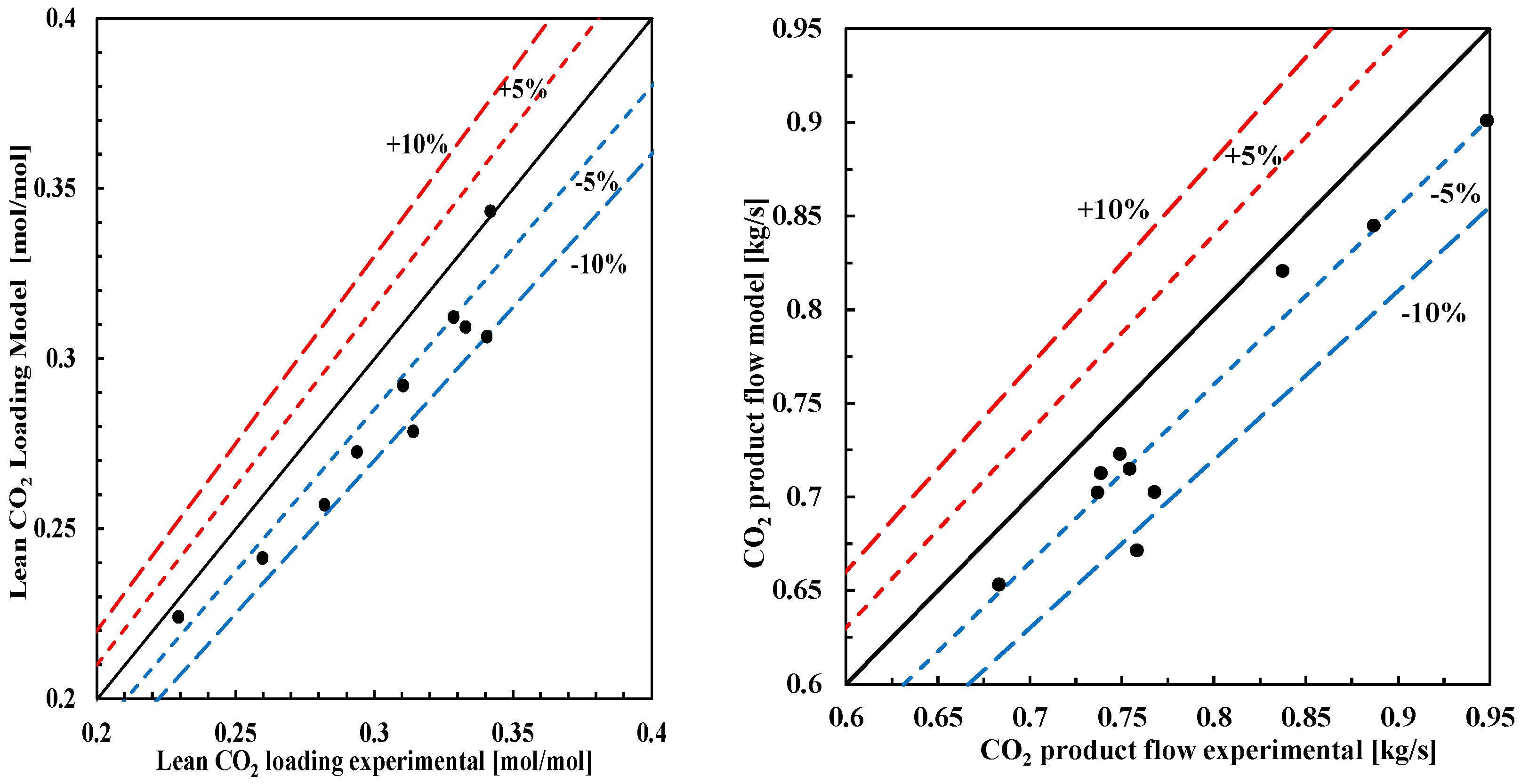
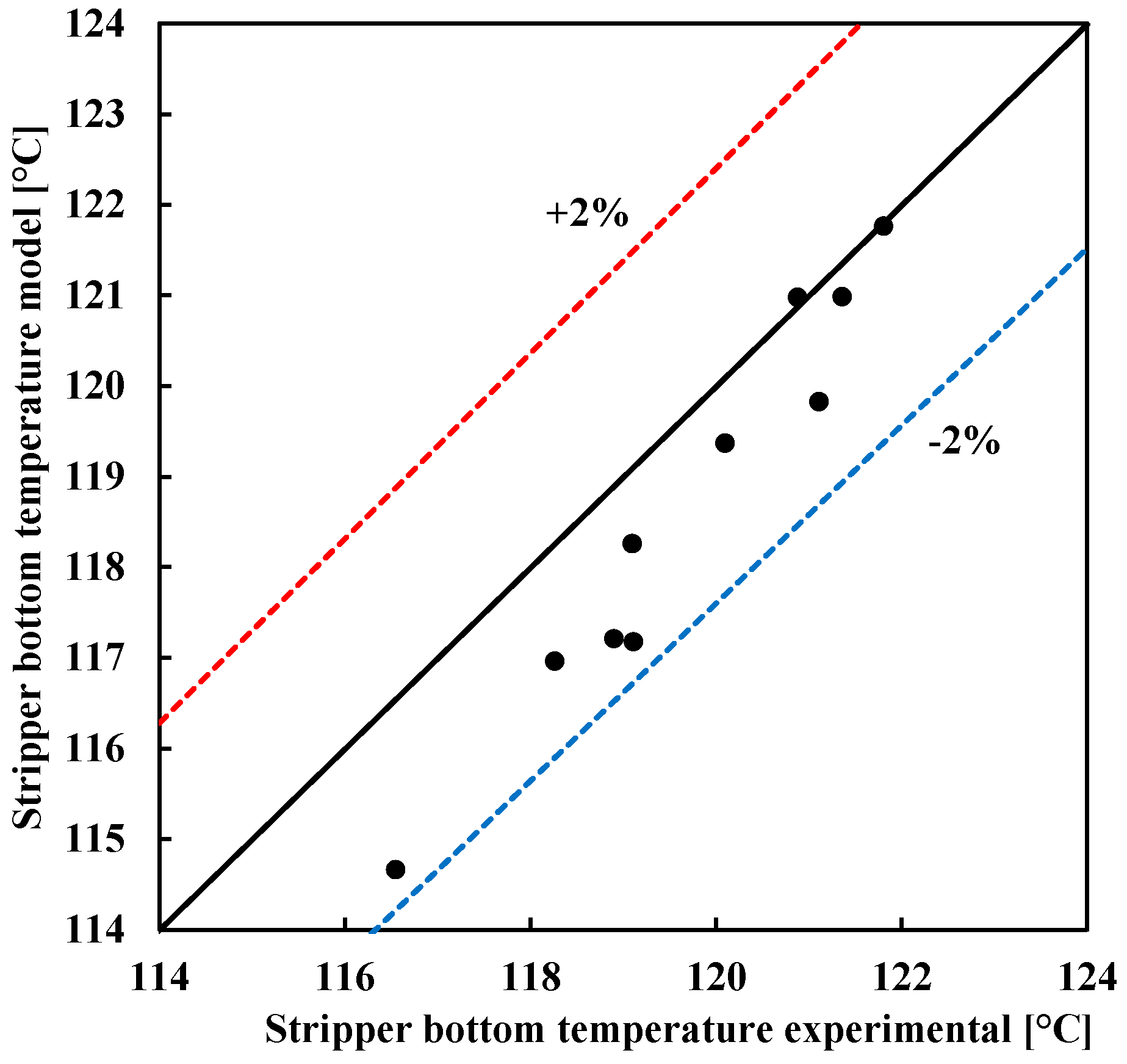
The results for lean CO2 loading are presented in Figure 2 with a parity plot, where ±5% and ±10% error lines are also shown. It is clear that the dynamic process model under-predicts lean loading for most of the cases, with a MAP < 6.6%. In addition, Figure 2 shows the parity plot for CO2 product flow rate; in this case, the CO2 product flow rate is also under-predicted by the dynamic process model, with a MAP < 5.3%. Figure 3 shows the parity plot for stripper bottom temperature, with the ±2% error lines plotted; stripper bottom temperature Tstr presented a MAP < 1%. From the parity plots, one can observe that, despite the errors found in the absolute values predicted by the dynamic process model with respect to the reference plant data, the dynamic process model can predict the variability in the main process variables for a wide range of steady-state operating conditions.
Temperature within absorber and stripper column is an important process variable since it affects phase equilibrium at liquid and gas-liquid interface. Some important model parameters and thermophysical properties depend on temperature, including heat capacity, water heat of condensation, heats of reaction, equilibrium constants and CO2 solubility. Therefore, it is desirable that the dynamic process model can predict with good accuracy absorber and stripper columns’ temperature profiles. Figure 4 shows the comparison between the pilot plant temperature profiles of the absorber and desorber columns with the predictions from the simulation of the dynamic process models. Two steady-state operating cases are presented: Case 1 (Table 3) with absorber flue gas volumetric capacity of 100%, mass-based L/G ratio of 0.89 and capture target of 85%; and Case 6 (refer to Table 3) with 80% flue gas volumetric capacity, mass-based L/G ratio of 1.34 and capture target of 85%. Both cases were operated with 24 m of wet absorber packing, and represent two operating cases with different flue gas capacities and L/G ratios.
Validation of absorber and stripper temperature profiles is normally considered a challenging task for several reasons. At TCM DA the temperature profiles are the resulting averaged values of the 4 measurements distributed radially in a given axial position within the column; refer to Section 3. A given pilot plant temperature value presented in Figure 4 is the resulting average over time during one hour of steady-state operating conditions, of the averaged 4 temperature measurements radially distributed within the absorber or stripper column, at the given axial position of the column. The individual temperature measurements are considered reliable and the resulting temperature profiles are reasonable. However, some sensors are located closer to the center of the packing while others closer to the wall. This results in a maximum variation (<6 °C) which is observed between the measurements in the same radial plane, which depends on operating conditions and is different at different radial planes. Based on the results presented in Figure 4, the dynamic process model can properly predict absorber and stripper column temperature profiles with sufficient accuracy considering the purpose of application. Absorber temperature profiles predicted by the model show a good agreement with the experimental pilot plant data, and the model is capable of properly predicting the trends in temperature along the column. The absorber temperature profiles have a mean absolute percentage error (<2.5%) for Case 1 and (<2.1%) for Case 6, which is within the observed maximum variability of the temperature measurements in a given radial plane. In addition, desorber temperature profiles have a mean average error (<0.6%) for Case 1 and (<3.6%) for Case 6. It is the desorber temperature profile for Case 6 that presents the less accurate prediction. In addition, it can be concluded that the process model is capable of properly predicting the variation of temperature profiles for various steady-state operating conditions.
4. Validation of Dynamic Process Model with Transient Plant Data
For dynamic process model validation purposes transient tests are conducted by means of open-loop step changes in the main process inputs to the plant. The transient behavior occurs between the initial steady-state operating conditions until the new steady-state operating conditions are reached. In this work, the experiments consist of set-point changes in rich solvent flow rate, flue gas volumetric flow rate fed to the absorber and reboiler duty. The output trajectories of main process variables are observed and compared with the model output trajectories. In order to obtain good sets of data for validation, it is desired to apply the step changes in plant inputs in a non-simultaneous manner. However, this is not normally easy to implement in practice. In order to compare the pilot plant experimental output trajectories with the output trajectories predicted by the dynamic process models, input trajectories were utilized in the dynamic simulations. This means that the measured time series of the inputs applied to the pilot plant during the tests were applied as disturbances or inputs to the dynamic process model; refer to Figure 5a, Figure 6a and Figure 7a. During the three tests, the regulatory control layer of the plant was active. In Figure 5 and Figure 6, the time t = 0 corresponds to the point from which the set point of flue gas volumetric flow rate was changed. In Figure 7 the time t = 0 is the point from when the set point of rich solvent flow rate was changed.
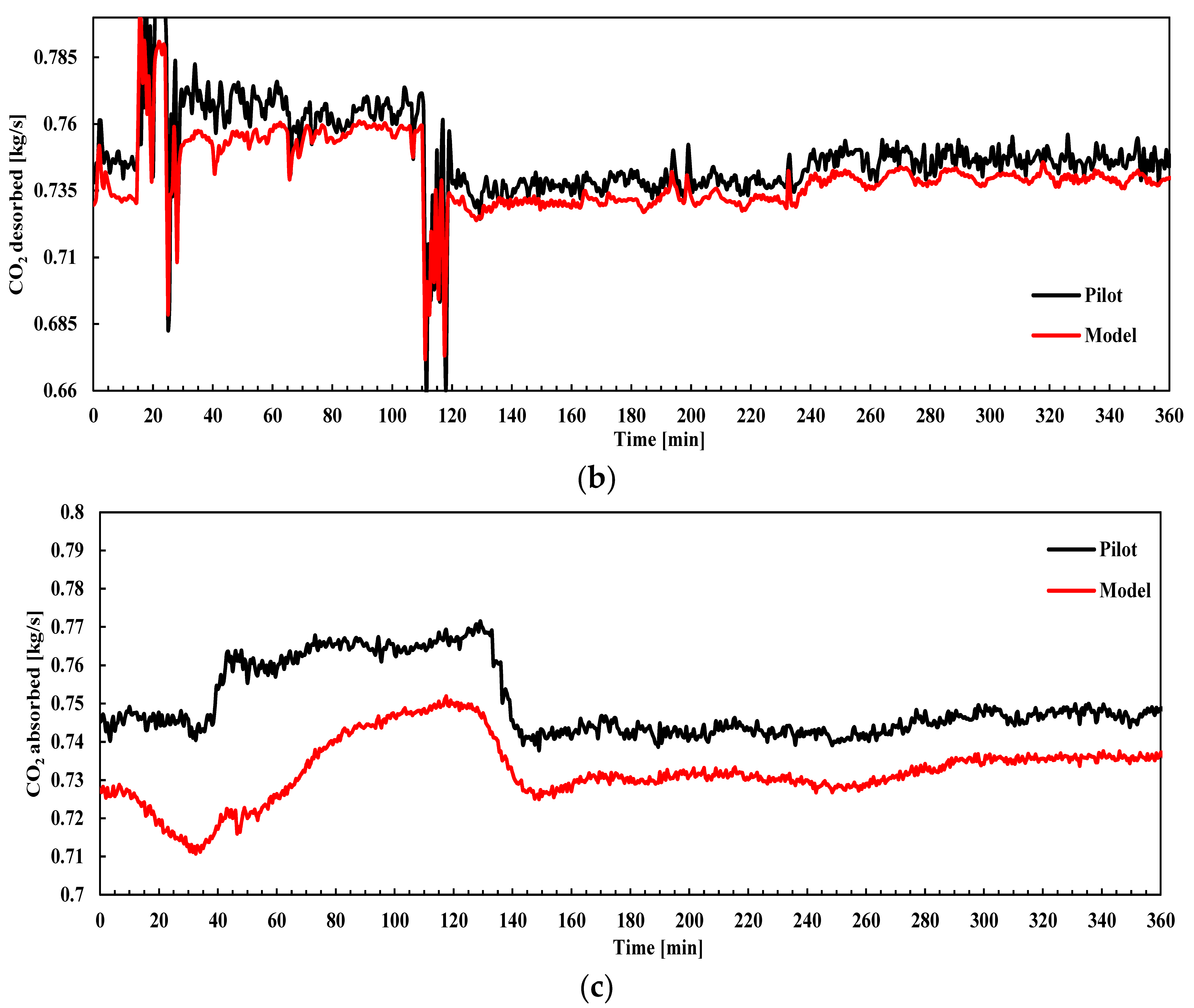
4.1. Flue Gas Flow Rate Ramp-Down
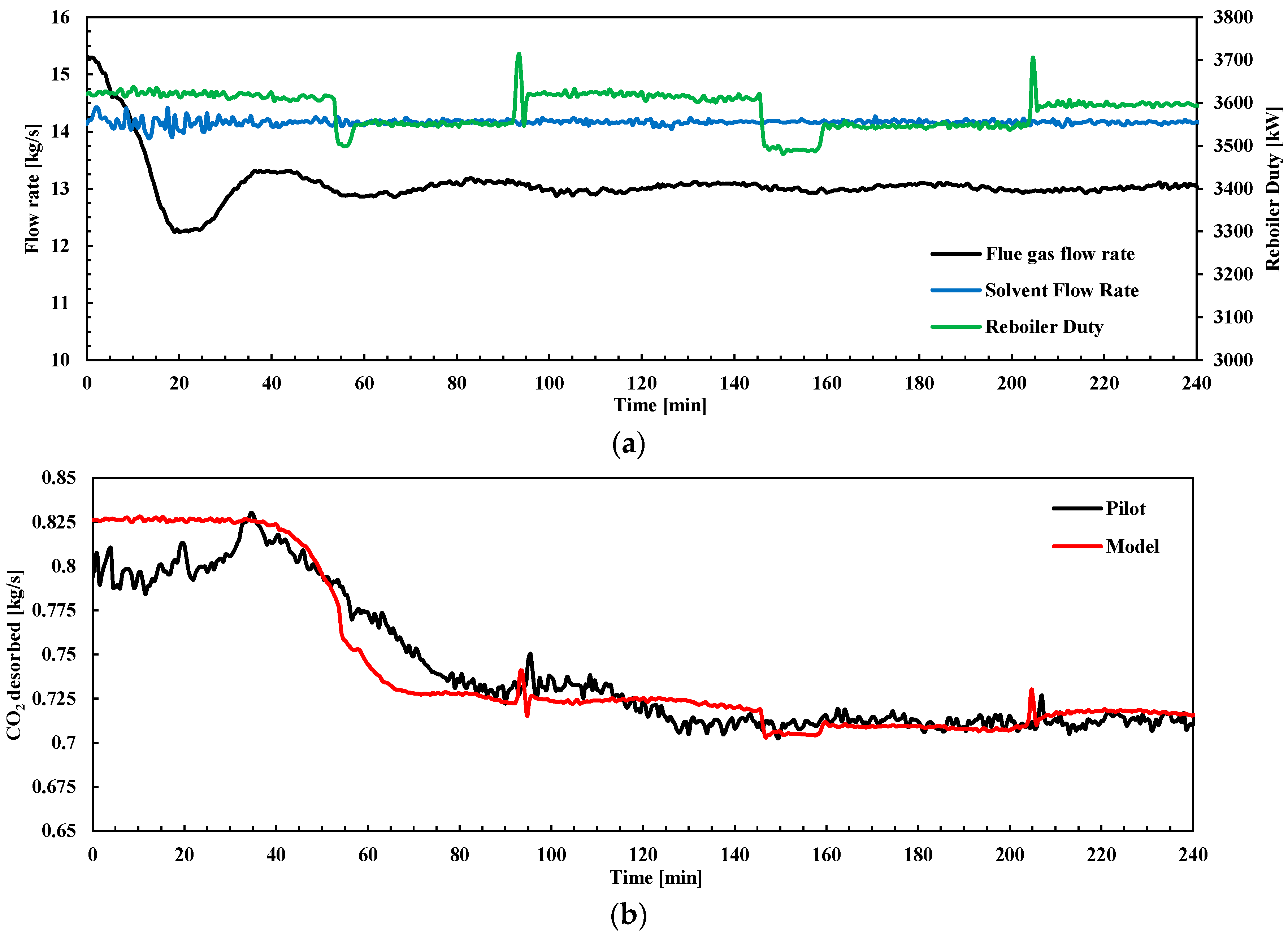
The main disturbance applied in this transient test consisted of a reduction in flue gas volumetric flow rate at the inlet of the absorber. It was implemented at TCM DA pilot plant by changing the set point of the blower cascade controller from 47,000 Sm3 to 40,000 Sm3; refer to FT1 in Figure 1. This corresponds with flue gas volumetric flow capacities in the absorber column of 80% and 67% respectively. Figure 5a shows the three main inputs of the plant for this test. During the test, reboiler duty was changed in steps around the value of 3550 kW; this might be due to the effects of the regulatory control layer on steam mass flow rate. The solvent mass flow rate had small amplitude oscillations around the set point.
Figure 5b,c show the output trajectories of CO2 product flow rate (or CO2 desorbed) and CO2 absorbed to the disturbance applied in this test. CO2 absorbed is calculated as the difference between CO2 mass flow rate at the absorber inlet and the CO2 mass flow rate leaving the absorber with the depleted flue gas at the top of the absorber; refer to Equation (12). In Figure 5b, a dead time of around 40 min was observed, i.e., no significant changes are found in the CO2 desorbed until around 40 min after the disturbance was applied to the pilot plant. In addition, the plant did not reach steady-state operating conditions until around 4 h later. As shown in Figure 5c, there is not significant dead time in the response of CO2 absorbed. The difference observed between the output trajectories is characteristic of the coupled transient performance of the absorber and stripper columns. Figure 5b,c shows that the process model is capable of predicting the main process dynamics for CO2 product mass flow rate (CO2 desorbed), including an adequate prediction of dead times and stabilization time. In addition, the CO2 absorbed transient performance trends are predicted in a satisfactory manner.
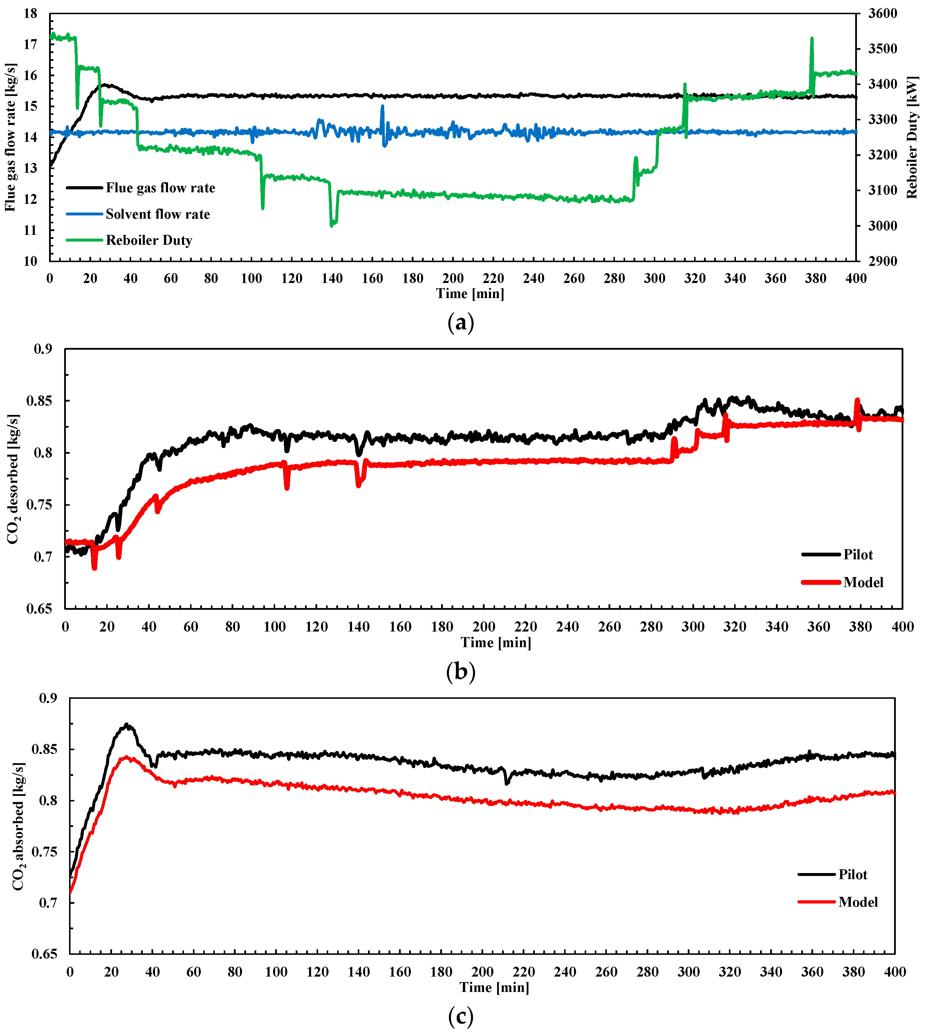
4.2. Flue Gas Flow Rate Ramp-Up and Step Changes in Reboiler Duty
These tests consist of combined input changes to the plant in terms of flue gas volumetric flow rate and reboiler duty. A set-point increase of the flue gas volumetric flow rate fed to the absorber from 40,000 to 47,000 Sm3/h was applied. This corresponds with 67% and 80% of the absorber column capacity, respectively. In addition, step-changes in reboiler duty were applied during the transient test. Figure 6a shows the three main inputs of the plant during the test. Figure 6b,c show the CO2 product flow and CO2 absorbed for the model and the pilot plant data. In this test a dead time of around 20 min in the response of CO2 desorbed was observed. This confirms the buffering effect by the chemical process in terms of the response of CO2 desorbed when the flue gas volumetric flow rate is changed. There is evidence to support this observation in previous pilot plant studies [46,47,48]. The delay in the response is partly attributed to solvent circulation time and the redistribution of liquid. Despite the steady-state offset shown on CO2 absorbed in Figure 6b, a good prediction of the main transient response is seen. It is possible that the reduction in reboiler duty at around 10 min flattens out the response in CO2 product flow rate.
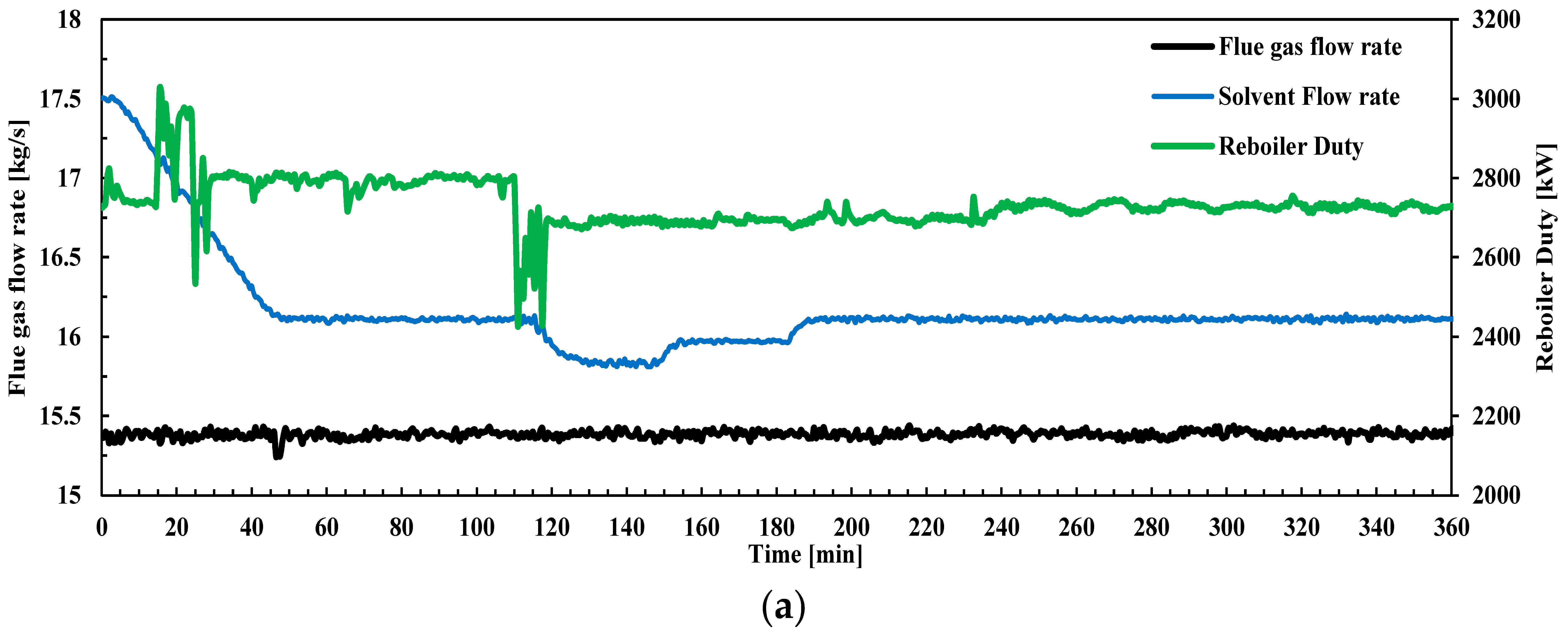
4.3. Solvent Flow Rate Ramp-Down
In this test, the plant is operated in steady-state until the rich solvent mass flow rate set point is ramped down from around 17.5 kg/s to around 16.1 kg/s; refer to FT5 in Figure 1. The reboiler duty and flue gas volumetric flow rate were intended to be kept constant. Figure 7a shows the three main inputs of the plant during this transient test. In addition, the pilot plant performance in terms of product CO2 mass flow Fprod (or CO2 desorbed) and absorbed CO2 flow rate are presented, together with the dynamic process model simulations for this test. Again, a satisfactory agreement is found between the plant trajectories and the output trajectories predicted by the dynamic process model.
From the three transient tests presented above, it can be concluded that the dynamic process model predicts the transient trends of the main output trajectories of the process for different inputs to the plant. In addition, the dead times and stabilization times of the process are properly predicted by the dynamic process models, despite the steady-state deviations observed and already quantified in Section 3.2. This means that the dynamic process model is suitable for simulation studies at the plant scale, including dynamic process simulations to analyze the plant transient performance, and for control tuning and advanced control layer design, including control structure studies.
5. Case Study: Open-Loop Performance and Decentralized Control Structures
5.1. Open-Loop Step Responses at Different Plant Flue Gas Capacities
A power plant operated in a power market with a high penetration of renewables will most likely be operated in load-following mode [7,63]. This means that the power plant with PCC will be operated during a significant amount of its lifetime at part loads. In the case of a natural gas combined cycle power plant with post-combustion CO2 capture it means that, at part-load operation, the gas turbine (GT) load will be reduced, generating a reduced mass flow rate of flue gas that would be conducted to the PCC unit. The purpose of this case study is to investigate the transient performance of the PCC pilot plant via dynamic process simulation by implementing open-loop step changes to the dynamic process model, and to compare the response of the plant at different part-load operating points, defined by different mass flow rates of flue gas to be treated. The analysis will assess the transient response of the plant to multiple and non-simultaneous step changes in three key inputs to the plant, namely (i) flue gas flow rate Fgas (ii) solvent flow rate Fsolv; and (iii) reboiler duty , at different flue gas mass flow rate capacities of the plant. In order to define the part-load operating points, a decentralized control structure was utilized, in which reboiler duty was the manipulated variable to control stripper bottom temperature Tstr to 120.9 °C, and the solvent flow rate was the manipulated variable to control CO2 capture ratio Cap to 0.85, as defined in Equation (13). When operating the plant at different flue gas mass flow rates, corresponding to 100%, 80% and 60% of nominal mass flow rate, this results in the three steady-state operating points presented in Table 5 and Table 6. The control structure is defined as control structure A in Table 7.
The open-loop response was studied for the process variables (i) CO2 absorbed CO2,abs, in Equation (11); (ii) CO2 desorbed CO2,des (or Fprod); (iii) lean CO2 loading Ll at the inlet of the absorber; and (iv) rich CO2 loading Lr at the outlet of the absorber. To characterize the transient response, dead time θ, settling time ts, total stabilization time tt, and relative change (RC) were calculated:
- Dead time θ: it is the time that takes before a process variable starts to change from the initial steady-state conditions as a response to the disturbance or input.
- Settling time: The 10% settling time ts is the time taken from when the process variable begins to respond to the input change (dead time) until it remains within an error band described by 10% of the change in the process variable Δy and the final steady-state value of the process variable y∞, i.e.: −0.1 Δy + y∞ < y∞ < 0.1 Δy + y∞.
- Total stabilization time: the sum of the dead time θ and the settling time ts is the resulting total stabilization time tt.
- Relative change RC: Change in the observed process variable from initial steady-state conditions y0 to the final steady-state conditions; refer to Equation (14).
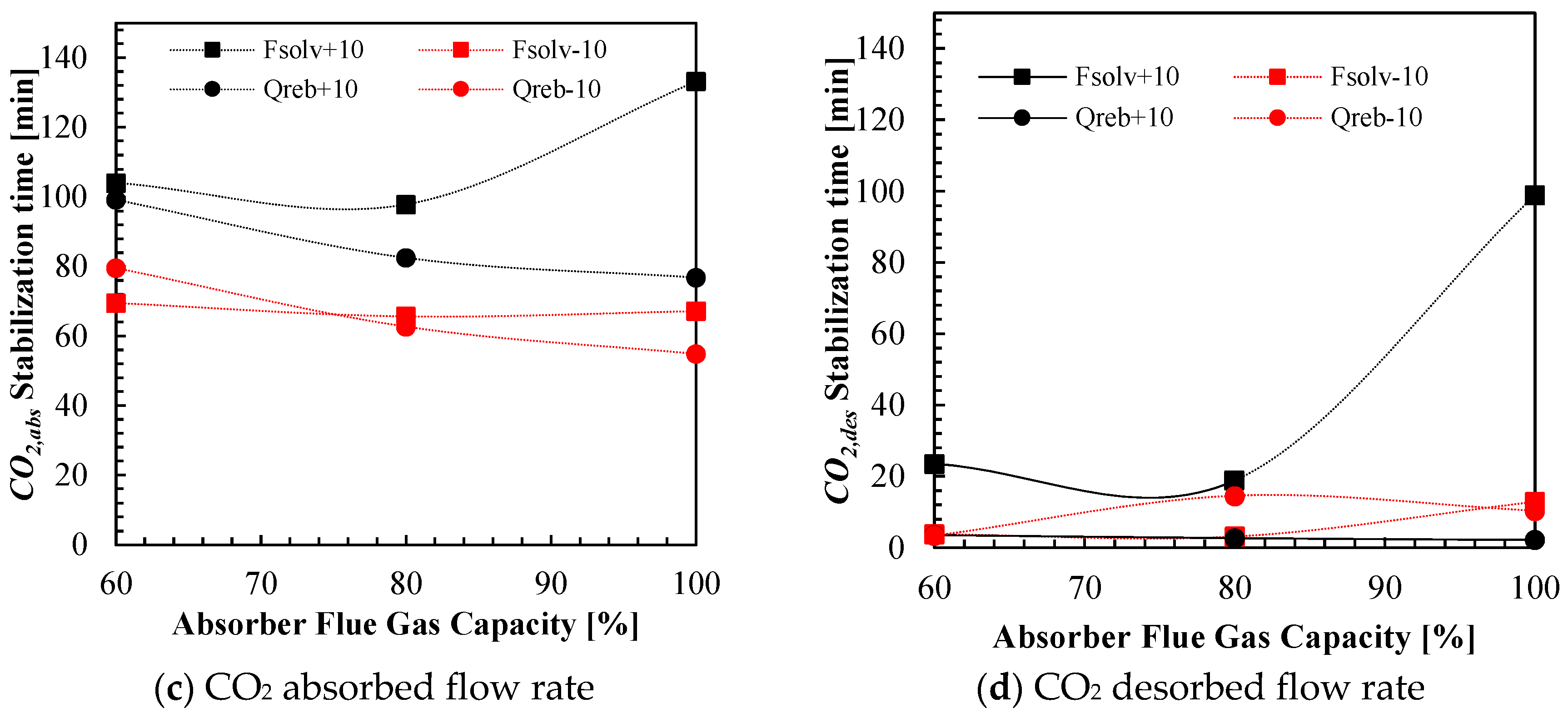
The detailed results of the process simulations are presented in Table A1, Table A2 and Table A3 in Appendix A. Figure 8 shows the total stabilization times for the selected process variables at the three operating points, for step changes in solvent flow rate and reboiler duty. The responses for step changes in flue gas flow rate are not presented, since it is shown in Table A1 that the relative change RC in the output process variables is very small or negligible (RC ranges from −0.81% to 0.21%). This can be explained by the highly diluted nature of the CO2 in the flue gas (ca. 3.5 vol%). The results show the non-linear behavior of the plant, with different transient responses to step change set-point increase and decrease in key plant inputs, and at different loads of the plant.
Figure 8a shows the total stabilization time for lean CO2 loading Ll at the inlet of the absorber, which ranges from 25 to 45 min in all cases. The results show that the required time for total stabilization increases when the plant is operated at lower loads. As shown in Appendix A (Table A1 and Table A2), a general trend was that the dead time θ in the response of Ll to step changes in reboiler duty and rich solvent mass flow rate increases at part-load points. This could be explained by the fact that at lower loads the solvent mass flow rate is smaller (refer to Fsolv in Table 6), resulting in longer residence times of the solvent through each equipment hold-up, piping, and recycle loop, this is, larger circulation time. This can also explain why dead times are generally larger when decreasing solvent flow rate than when increasing it; refer to Table A2 in Appendix A.
Figure 8b shows the total stabilization times for rich CO2 loading Lr at the outlet of the absorber sump. In this case, the stabilization times range from 60 to 450 min. It should be mentioned that the relative change RC in rich CO2 loading is also small or negligible for the disturbances studied (see Appendix A), due to the fact that the solvent is operated close to its maximum loading capacity of 0.51 mol/mol CO2 loading. The total stabilization times of the responses of rich CO2 loading Lr to disturbances in solvent flow rate and reboiler duty are larger at lower plant loads. At 60% flue gas capacity, a very slow response is found in Lr when the solvent flow rate is decreased by a −10% step change; however, the relative change RC of Lr in this process variable is negligible for this plant disturbance; refer to Table A2 in Appendix A.
The total stabilization times for CO2 absorbed CO2,abs response to disturbances in rich solvent mass flow rate Fsolv and reboiler duty reb are shown in Figure 8c. Total stabilization times range from 55 to 135 min. When the rich solvent mass flow rate is increased by 10%, this results in an increase in CO2 absorbed with a relative change RC of 0.35% to 4.18% (refer to Table A2), due to the increased L/G ratio in the absorber column. However, since the reboiler duty is kept constant, the lean loading will increase (see RC values of Ll in Table A2). Due to the residence time in the hot solvent piping, lean/rich heat exchanger and lean amine cooler of the recycle loop, it takes time for the solvent to be distributed towards the inlet of the absorber. A dead time in CO2 lean loading Ll at the inlet of the absorber of 11 to 22 min is observed (see Table A2). This results in it taking a long time for the CO2,abs to stabilize. When the rich solvent mass flow rate is decreased by 10%, it is observed that the CO2 absorbed CO2,abs decreases (relative change RC between −3.14% and −5.59% in Table A2). This is a result of the combination of the reduction in L/G ratio and the decrease in lean loading Ll. CO2,abs requiring time for stabilization (stabilization time of 65 to 69 min). When reboiler duty reb is increased by 10%, the lean loading Ll is decreased significantly (RC ranging from 6.75 to 8.59%), which results in increase of CO2,abs (relative change RC of 4.0% to 6.07%). The change in lean loading Ll is observed at the absorber inlet with a dead time of 13 to 23 min (due to circulation time of the solvent in the recycle loop), and the total stabilization time for CO2,abs for increase in reboiler duty ranges from 76 to 99 min. When reboiler duty reb is decreased by 10%, the solvent lean loading increases (RC of 6.63% to 8.46%), resulting in less CO2 being absorbed. Relatively slower response in CO2,abs to disturbances in solvent flow rate and reboiler duty were found when the PCC was operated at lower loads (55 to 99 min). An exception is found for the case when the solvent flow rate is increased at 100% mass flow rate operating conditions of the plant.
Figure 8d shows the stabilization times for CO2 desorbed CO2,des. For disturbances in rich solvent flow rate and reboiler duty, the desorbed CO2 stabilizes slightly faster at lower loads (ranging from 2 to 100 min). In general, it was found that the desorption rate stabilized faster than the absorption rate CO2,abs for the disturbances in solvent flow rate and reboiler duty applied to the process. When solvent flow rate is decreased, this results in smaller L/G ratio in the absorber column and less CO2 being desorbed in the stripper column. Since the rich CO2 loading does not change significantly (RC in Lr from 0 to 0.08%), the CO2 desorbed CO2,des stabilizes faster than the CO2 absorbed (circulation time through the recycle loop is not affecting the stabilization of CO2,des). When the reboiler duty reb is increased by 10%, the relative change in CO2 desorbed is large (4 to 6.07% in Table A3), and with fast total stabilization time (2 to 3 min in Table A3). A change in reboiler duty results in a fast response in the produced stripping vapors, which also results in a fast response in CO2 product flow rate (CO2 desorbed). The longest stabilization time for CO2 desorbed is found when the solvent flow rate is increased at 100% operating conditions. It is notable that there is a big difference in total stabilization times for solvent flow rate increase at different loads of the plant.
5.2. Decentralized Control Structures
In this section, four control structures for the TCM DA amine plant were tested via dynamic process model simulations. The scenario considers realistic load changes on the power plant, by changing flue gas flow rate feed to the absorber column. From a control analysis perspective, flue gas flow rate change can be considered as a disturbance applied to the PCC process. A load change event would result in a significant change in flue gas flow rate, at a ramp rate given by GT operation and controls. Fast ramp rates are the goal of power plant operators, since a fast power plant can respond to the variability in costs in a day-ahead power market [7,64]. For a NGCC power plant, a fast ramp rate is considered to be around 10%/min GT load [4,65]. Two tests were considered and simulated:
- Test 1: Ramping down flue gas flow rate from 100 to 70% in 3 min. The transient event starts at t0 = 0 min, and sufficient simulation time is allowed for the plant to reach the new steady-state.
- Test 2: Flue gas flow rate is ramped up from 70 to 100% in 3 min. The transient event starts at t0 = 0 min, and sufficient simulation time is allowed for the plant to reach the new steady-state.
The supervisory or advanced control layer of the TCM DA amine plant has three main degrees of freedom, consisting of set point of flue gas volumetric flow rate Fgas, set point of rich pump solvent flow rate Fsolv, and steam flow rate to feed the reboiler duty ; refer to FT1, FT5 and FT4, respectively in Figure 1. Under normal and stable operation of the pilot plant at TCM DA, such degrees of freedom are changed manually by the operators to bring the plant to different operating conditions. If flue gas flow rate is considered to be a disturbance, there are two degrees of freedom left for operation. Note that here we do not consider the degrees of freedom available to the operators in the stabilizing or regulatory control layer, or for other auxiliary operations of the plant, or start-up procedures. Several studies in the literature suggest that keeping the capture ratio Cap and a temperature in the stripper column constant can lead to efficient operation of the process for varying loads of the PCC absorber-desorber process [13]. In this analysis, four control structures were tested, as presented in Table 7. All the feedback control loops are PI controllers, and were tuned with the simple internal model control (SIMC) tuning rules [66].
- Control structure A uses Fsolv to control capture ratio at the top of the absorber Cap defined by Equation (13) to the set point of 0.85, and reboiler duty reb to control the solvent temperature at the stripper bottom Tstr to the set point of 120.9 °C. This control structure has been previously proposed in the literature in different studies including [14,16], where it shows a fast response and the capability to reject disturbances.
- Control structure B uses Fsolv to control the solvent temperature at the stripper bottom Tstr to the set point of 120.9 °C, and reboiler duty reb to control capture ratio at the top of the absorber Cap to the set point of 0.85. Note that changes in reboiler duty result in a big change in solvent lean CO2 loading (large relative change RC; see Appendix A). A similar version was suggested by Panahi and Skogestad [14], where it was found that this control structure showed similar dynamic behavior, in response to disturbances in flue gas flow rate, compared with a model predictive control scheme (MPC).
- Control structure C utilizes solvent flow rate Fsolv to control the mass-based L/G ratio in the absorber column at the same value as that in the close-to-design-point operating conditions. This control structure has been studied previously in [12,15]. This control loop is implemented via ratio control. In addition, reboiler duty is manipulated to control Tstr to 120.9 °C. The control structure leads to different final steady-state operating conditions when ramping down the plant load than the other three alternatives.
- Control structure D is a modification of control structure A. In this control structure, the solvent flow rate set point is changed via a feed forward (FF) action to control the capture ratio Cap at 0.85; in addition, the stripper bottom temperature is controlled by manipulating the reboiler duty. The feed forward controller is implemented by a set-point ramp change in the solvent flow rate with the same total duration as the flue gas flow rate ramp change, to the final value that gives a Cap of 0.85 under final steady-state conditions.
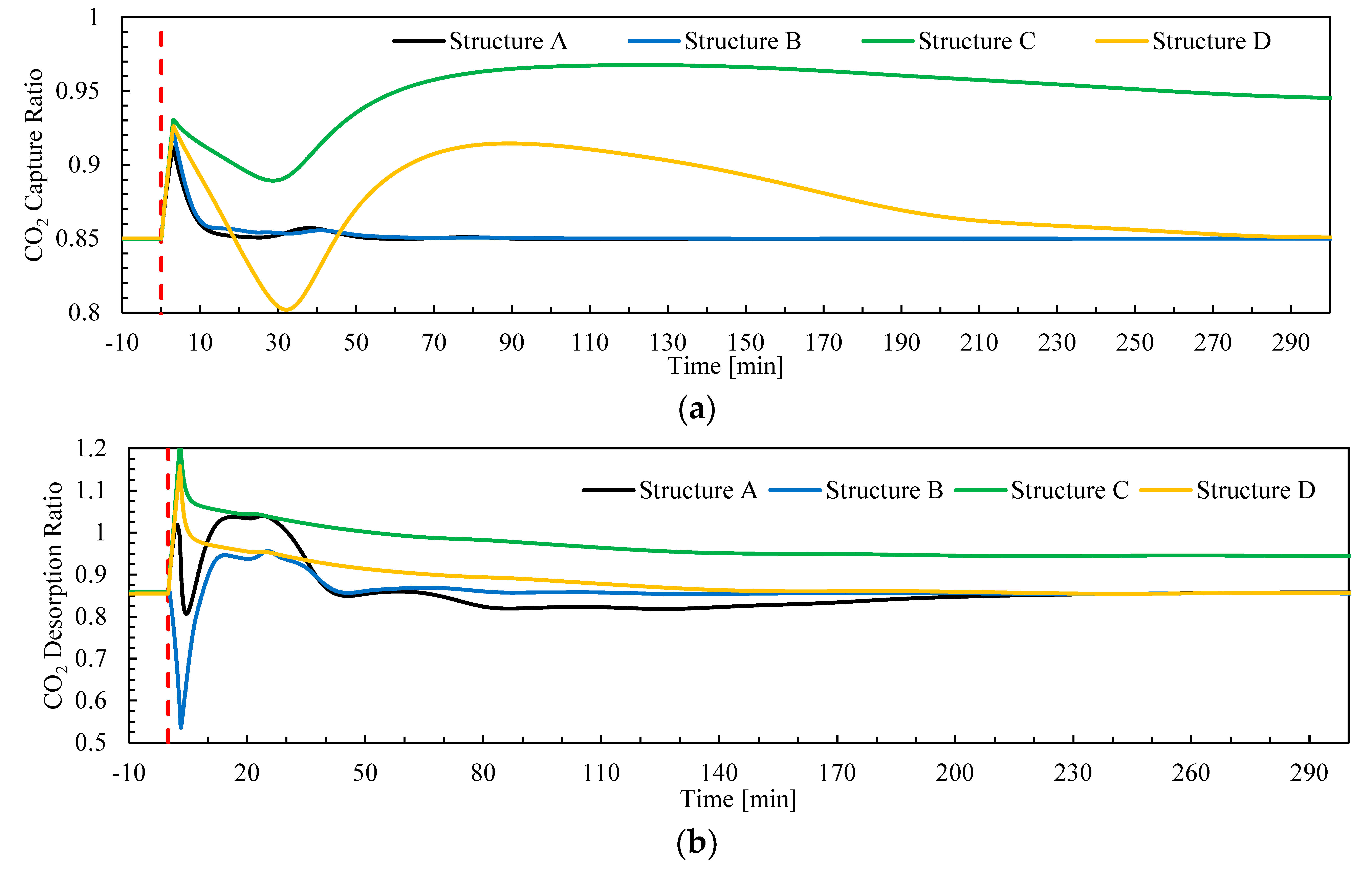
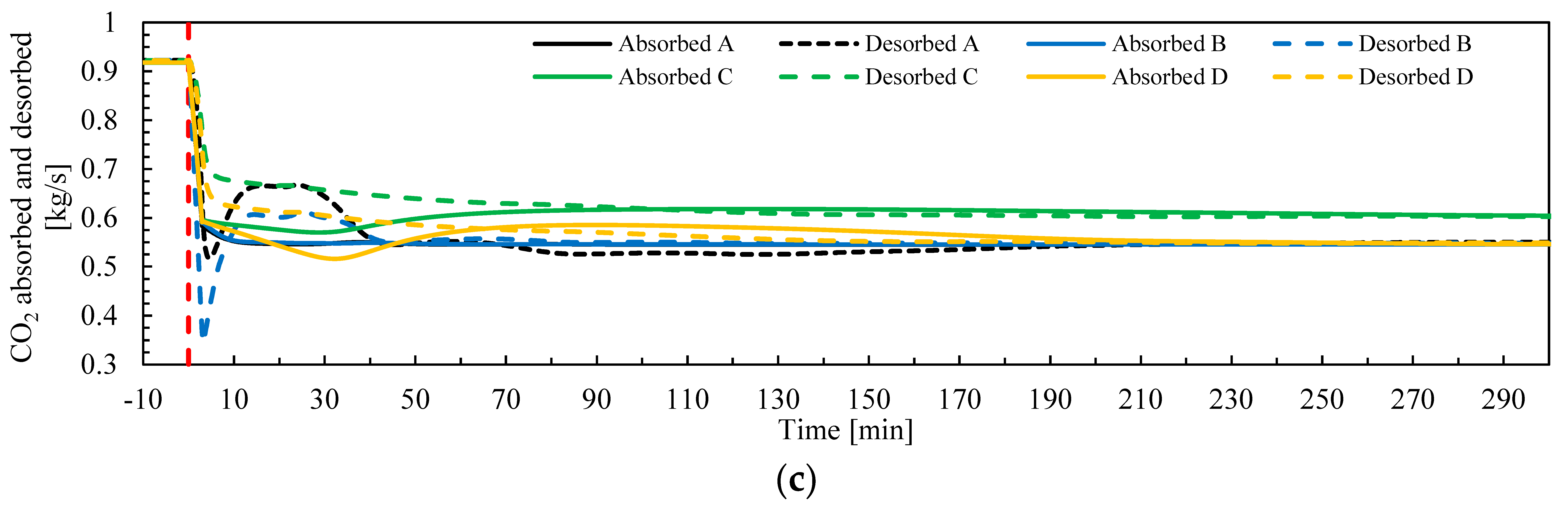
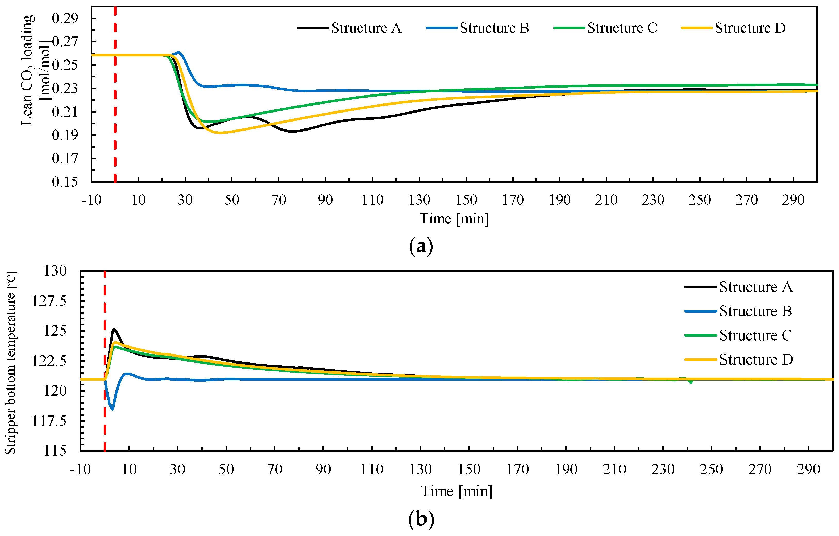
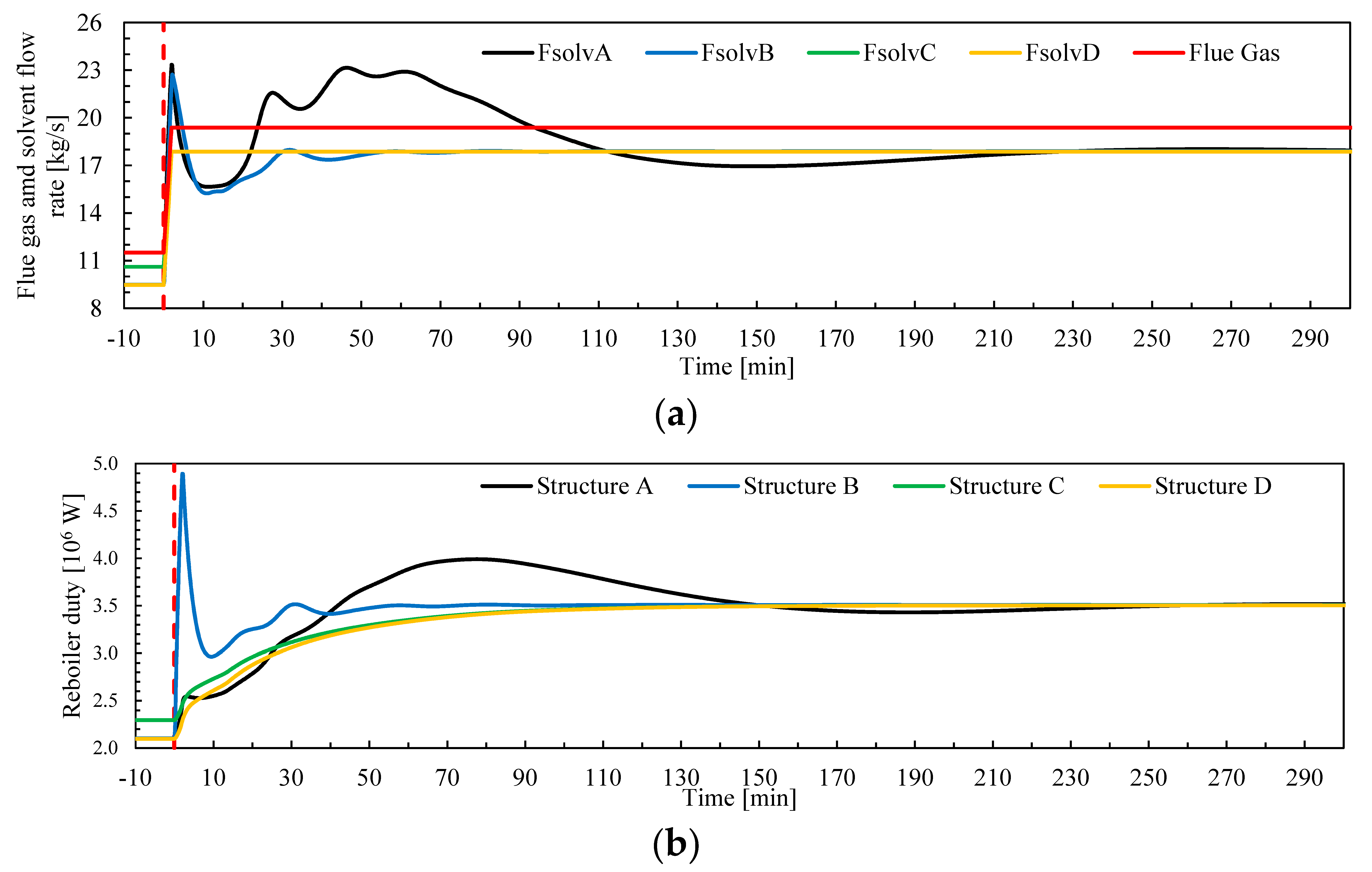
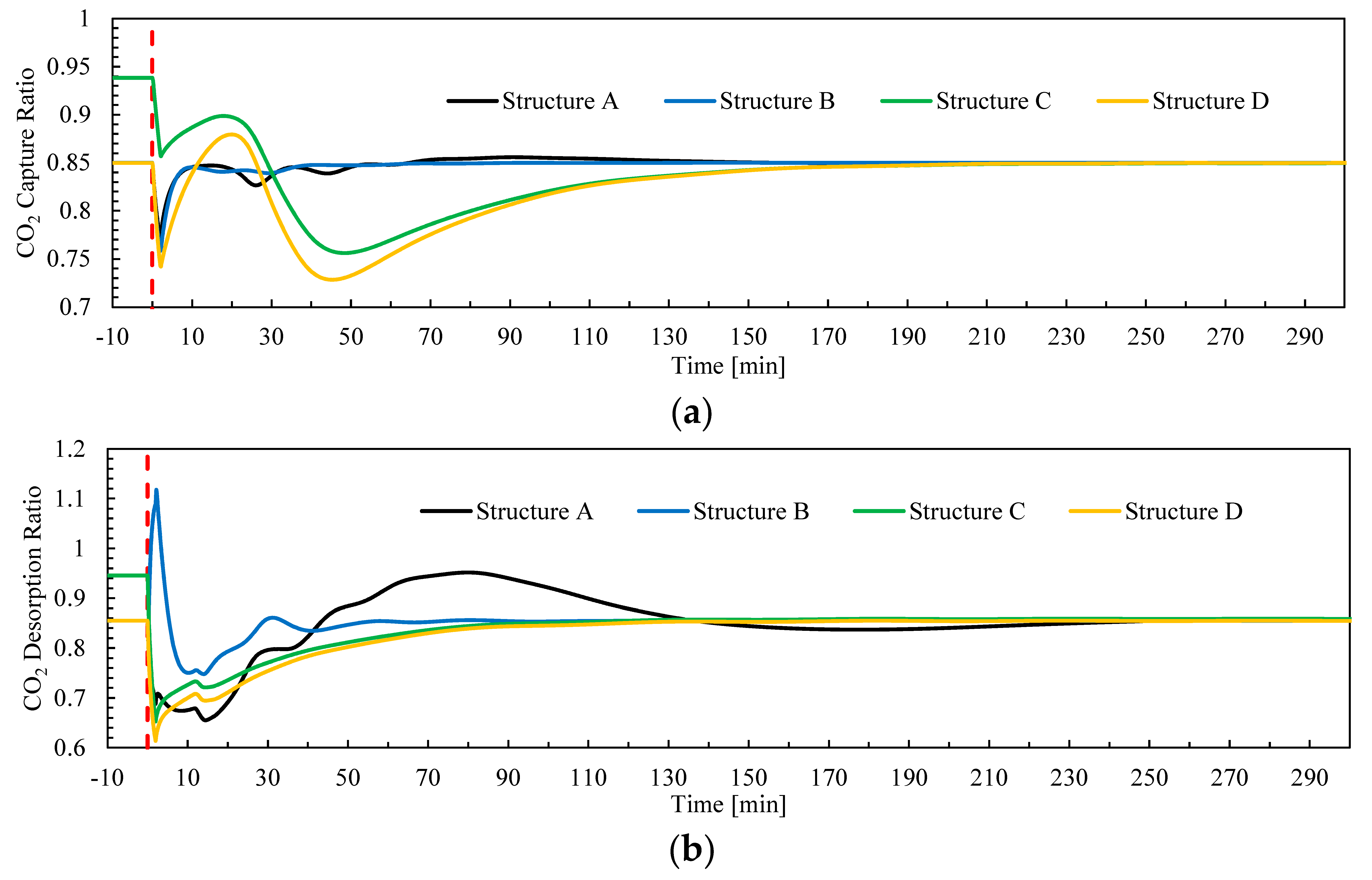
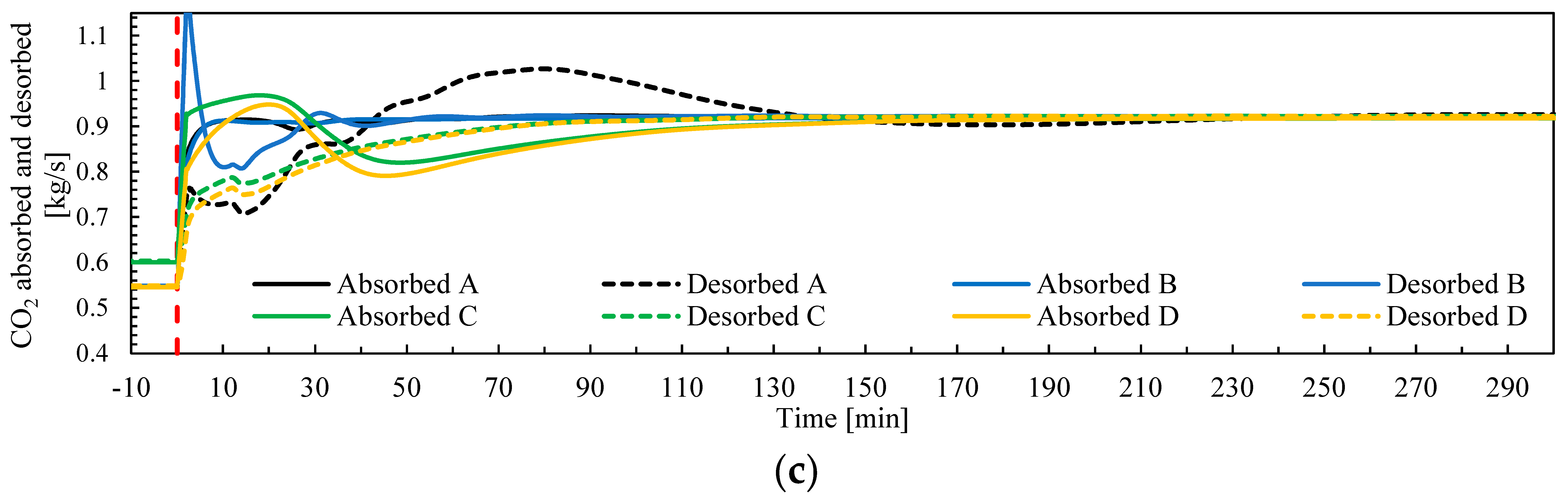
Figure 9 shows the simulated time input trajectories during the test with flue gas flow rate reduction. The manipulated variables Fsolv and are shown for the different control structures evaluated. Figure 10 shows the output trajectories of CO2 capture ratio Cap, desorption ratio Des, CO2 absorbed and CO2 desorbed for the transient tests of flue gas flow rate reduction. Figure 11 shows the trajectories of lean loading Ll and stripper bottom solvent temperature Tstr for flue gas flow rate reduction. In addition, Figure 12 shows the simulated time input trajectories during the test with flue gas flow rate increase. Figure 13 shows the output trajectories of CO2 capture ratio Cap, desorption ratio Des, CO2 absorbed and CO2 desorbed for the transient tests of flue gas flow rate increase, and Figure 14 shows the trajectories of lean loading Ll and stripper bottom solvent temperature Tstr for flue gas flow rate increase. In order to compare the different control structure performances during transient load change, the total stabilization times of the selected process variables are shown in Table 8. These will indicate how fast the plant achieves stabilization of the different floating (not controlled) process variables when moving from one operating condition to the next one. In addition, three transient performance indicators have been considered and presented in Table 9. Note that, for this analysis auxiliary consumptions of the plant are not considered.
- Accumulated reboiler energy input Qreb (MJ): see Equation (15). This is calculated by integration of the trajectory under the transient event, from the initial time t0 = 0 min to the final time tf = 480 min (8 h). The final time was defined to ensure that the plant was already under steady-state conditions at the final operating point. This value Qreb represents the main energy consumption of the process during the transient event of load change. In addition, the consumption of an ideal static plant is included for comparison (see Table 9). The ideal static plant is assumed to change from initial to the final steady-state operating conditions instantaneously at time t0, and would operate until tf. The static plant value represents the minimum value when ramping down and a maximum value when ramping up.
- Accumulated CO2 emitted CO2,em (tons): see Equation (16). This is calculated by integration of the trajectory under the transient event, from the initial time t0 = 0 min to the final time tf = 480 min; this represents the CO2 emitted at the absorber stack. The final time was defined to ensure that the plant was already under steady-state conditions at the final operating point. This measure represents the CO2 emitted during the transient event of load change. For comparison, the CO2 emitted by an ideal static plant is calculated (considered as the maximum value when ramping down and a minimum value when ramping up), shown in Table 9.
- Accumulated CO2 captured CO2,cap (tons): see Equation (17). This is calculated by integration of the CO2 absorbed CO2,abs trajectory (Equation (12)) under the transient event, from the initial time t0 = 0 min to the final time tf = 480 min. The final time was defined to ensure that the plant was already under steady-state conditions at the final operating point. This measure represents the CO2 captured during the transient event of load change. For comparison, the CO2 captured by an ideal static plant is calculated (considered as the minimum value when ramping down and a maximum value when ramping up), shown in Table 9.
Figure 10 shows that the CO2 capture ratio Cap had similar trajectories for control structures A and B during Test 1 (flue gas ramp-down), and that Cap reached stabilization conditions faster (20–50 min) than control structures C and D (around 270 min). Cap had also larger excursions from the set point than when control structures A and B are utilized. The same trends are found for Test 2 with flue gas flow rate ramp-up (Figure 13). When ramping up, control structures C and D stabilize faster (around 160 min) than when ramping down. This showed that the utilization of close-loop feedback control (structures A and B) allows shorter stabilization times to be reached for the controlled variable CO2 capture ratio Cap. The desorption ratio Des trajectories in Figure 10 show that the plant requires the shortest stabilization time for this process variable when employing control structure B (around 60 min), followed by control structure A and C (around 200 min). This can be explained by the fact that for a change in reboiler duty the response of CO2 desorbed has a fast total stabilization time and a large static relative change RC (where RC ranges from 4 to 6.29% and total stabilization time range from 2.2 to 3.5 min for a +10% step in reboiler duty); refer to Table A3. When it comes to the stabilization time required for Des for Test 1, structures C and D presented a poorer performance as the trajectories for Cap and Des deviate from the set point significantly. For control structure A, Des showed slow performance for Test 2 (around 210 min total stabilization time) with significant oscillations around set point; refer to Figure 13.
When ramping down the plant, CO2 absorbed and CO2 desorbed require similar stabilization times for control structures A and B (around 3 min for CO2,abs and 36 min for CO2,des), while the control structures C and D require longer stabilization times for CO2 desorbed (around 50 to 57 min); refer to Table 8. The trajectory of CO2 lean loading again shows shorter stabilization time for control structure B. This can be explained by the large static relative change RC of the response of CO2 lean loading to changes in reboiler duty (where RC ranges from −6.29% to −4.97% and total stabilization time range from 22.7 to 39.2 min for a +10% step in reboiler duty); refer to Table A3. This contributes to the tight control of CO2 capture ratio Cap achieved by control structure B, since the CO2 lean loading Ll is a key process variable that connects the operation of the stripper and the absorber columns via the recycle loop. In addition, control structure B shows the shortest stabilization times and smaller excursions of the stripper bottom temperature Tstr (around 15 to 30 min), in Figure 11 and Figure 14.
When the plant load is ramped up from 70 to 100% (Test 2), the control structure B in general showed a faster dynamic performance with significantly shorter stabilization times required for the floating process variables considered (5.2 min for CO2,abs, 27.5 min for CO2,des and 46.7 min for Ll), see Table 9; followed by C, D and A. Note that control structure B presented a faster dynamic performance towards stabilization while ramping up (Ll stabilizes in 46.7 min) than when ramping down the process (Ll stabilizes in 68.2 min). Control structures A, C and D required shorter stabilization times for CO2 absorption and CO2 desorption when ramping down the process load, while CO2 lean loading stabilized faster when ramping up the plant load; refer to the stabilization time values in Table 9. When the plant is operated under control structure C, the optimum solvent flow rate Fsolv and lean loading Ll are not reached at the 70% absorber capacity steady-state operating conditions; refer to time >250 min in Figure 9a and Figure 11a, and time <0 min in Figure 12a and Figure 14a. This leads to a higher Cap than specified (refer time t > 290 min in Figure 10a and time t < 0 min in Figure 13a), and therefore higher reboiler duty (time t > 290 min in Figure 9b and time t < 0 min in Figure 12b), even though the stripper bottom temperature Tstr criterion is satisfied.
During the ramp-down transient event of the plant (i.e., period of 8 h from the time change was implemented), the least energy-intensive performance measured by Qreb in Table 9 was observed for control structure B. In addition, this structure shows the largest CO2 emissions during the transient event, albeit still lower than the ideal static plant. The fast stabilization time of the plant process variables achieved by control structure B provides a transient performance that is the closest to the ideal static plant. Control structures C and D showed the largest CO2 captured during the transient event. However, when ramping down the plant load, this means that the plant is emitting less CO2 during the transient event with control structures A, B, C and D than that established by the operational objective and represented by the ideal static plant case. Consequently, when ramping down the plant load, CO2 emissions will always be lower than those of the equivalent ideal static plant. In addition, the plant is capturing more CO2 than the ideal static plant. Figure 10a shows how there are periods of time in which the capture ratio Cap is above the target of 0.85, leading to more CO2 being captured than the ideal static plant during the transient event. Control structures A and B showed the largest CO2 emitted when compared with the ideal static case. Despite control structure A presenting a similar amount of CO2 emitted during the transient event, it requires a larger amount of energy input during this period than control structure B. Therefore, control structure B shows the best performance in terms of energy consumption and CO2 emissions during the transient load change event of ramping down the PCC plant load. When ramping up the plant load the most energy-intensive control structure is control structure B. However CO2 emissions are the lowest, being closer to the minimum established by the static plant. This means that, when ramping up the plant load, CO2 emissions will always be higher than those of the equivalent ideal static plant. While control structure D is the least energy-intensive process during the transient event of load change increase, it is the control structure with the largest CO2 emissions during this transient event.
6. Conclusions
The pilot plant data obtained in this work from an MEA campaign at TCM DA amine plant includes ten steady-state operating data sets. The data sets consist of a wide range of steady-state operating conditions of the chemical absorption process in terms of L/G ratio in the absorber column, different absorber packing heights, CO2 capture ratios, reboiler duty and flue gas flow rate fed to the absorber. The data is considered reliable and valid and can be used for process model validation purposes. In addition, the three transient data sets presented in this work represent transient operation of the pilot plant driven by set-point changes in flue gas flow rate, solvent circulation flow rate and reboiler duty. The transient data sets are considered reliable and suitable for dynamic process model validation purposes, provided that input trajectories can be applied to the dynamic process model.
The validation of the dynamic process model with the steady-state and transient data shows that the process model has a good capability of predicting the steady-state and transient behavior of the plant for a wide range of operating conditions. The validation included in this work proves the capacities of dynamic process modeling applied to large-scale experimental data. The model is considered suitable for studies including transient performance analysis and control structure evaluation studies at the plant scale. In addition, it provides confidence towards using the dynamic process model for analysis of larger-scale PCC plants.
The case study carried out in this work via dynamic process simulations with the validated model shows that, generally, the plant responds more slowly at lower operating loads (the load being defined by the flow rate fed to the absorber). A general trend is observed, in which it takes a longer time to stabilize the main process variables of the pilot plant under open-loop step changes in the main inputs of the process, namely solvent flow rate, flue gas flow rate and reboiler duty. From the process simulations, it is found that, in general, the desorption rate stabilizes faster than the absorption rate for set-point step changes in solvent flow rate and reboiler duty. In addition, ±10% step changes in flue gas flow rate around a given operating point do not cause a large relative change in the main process variables of the process (RC ranges from −0.81% to 0.21%).
The evaluation of the decentralized control structures shows that by adding closed-loop controllers on the two main degrees of freedom of the plant—solvent flow rate and reboiler duty—to control two other process variables, including CO2 capture ratio and stripper bottom solvent temperature, the plant can be stabilized faster and more efficiently under varying loads. The control structure that showed the best performance was control structure B, in which the reboiler duty is manipulated to control CO2 capture ratio at the inlet of the absorber and the rich solvent flow rate to control the stripper bottom solvent temperature. It was observed that control structure B provides the fastest stabilization times for the main process variables under scenarios when the plant load is ramped down and up, with ramp rates typically found in NGCC power plants with fast-cycling capabilities. When reducing the PCC process load, this control structure is the least energy-intensive of those evaluated in this work. When increasing the plant load, this control structure is the one with the lowest accumulated CO2 emissions imposed by the process inertia during load-change transient operation.
Acknowledgments
The authors acknowledge the Department of Energy and Process Engineering at NTNU-Norwegian University of Science and Technology and TCM DA owners Gassnova, Shell, Statoil and Sasol, for funding this project. The funds for covering the costs to publish in open access were provided by the Norwegian University of Science and Technology—NTNU.
Author Contributions
Rubén M. Montañés contributed to the selection of experimental data; processed the experimental data; developed the models; carried out the calibration, validation and simulation of the dynamic process models; defined and carried out the case studies; analyzed the results; and wrote the manuscript. Nina E. Flø contributed to the experimental data selection; contributed to the critical analysis of the results; and reviewed the manuscript. Lars O. Nord contributed to the critical analysis of the results; reviewed the manuscript; and supervised the work.
Conflicts of Interest
The authors declare no conflict of interest.
Abbreviations and Symbols
| Aif | Contact area |
| AP | Absolute percentage error |
| Cap | CO2 capture ratio |
| CHP | Combined heat and power |
| CCS | Carbon capture and storage |
| CO2 | Carbon dioxide |
| CO2,em | CO2 emitted (kg/s) |
| ci | Molar concentration |
| Cef | Pre-multiplying coefficient |
| DCC | Direct contact cooler |
| Des | Desorption ratio |
| DCO2 | Diffusivity of CO2 in aqueous monoethanolamine |
| E | Enhancement factor |
| F | Mass flow rate (kg/s) |
| FB | Feedback |
| FC | Flow controller |
| FF | Feed-forward |
| FT | Flow transmitter |
| GA | Gas analyzer |
| GC | Gas chromatograph |
| GT | Gas turbine |
| Hei | Henry’s constant |
| H2O | Water |
| HX | Heat exchanger |
| ki | Mass transfer coefficient |
| Ki | Equilibrium constant |
| LC | Level controller |
| Ll | Lean CO2 loading |
| Lr | Rich CO2 loading |
| L/G | Mass-based liquid to gas ratio (kg/kg) |
| LT | Level transmitter |
| MAP | Mean absolute percentage error |
| MEA | Monoethanolamine |
| MPC | Model predictive control |
| N2 | Nitrogen |
| NCCC | National carbon capture center |
| NGCC | Natural gas combined cycle |
| O2 | Oxygen |
| p | Pressure (Pa) |
| PC | Pressure controller |
| PCC | Post-combustion CO2 capture |
| PT | Pressure transmitter |
| PZ | Piperazine |
| Reboiler duty (W) | |
| Qreb | Reboiler energy input (J) |
| RC | Relative change |
| SA | Solvent analyzer |
| SIMC | Simplified internal model control |
| SRD | Specific reboiler duty (kJ/kgCO2) |
| T | Temperature (K) |
| TC | Temperature controller |
| TCM DA | CO2 Technology Cener Mongstad |
| ts | Settling time |
| tt | Total stabilization time |
| TT | Temperature transmitter |
| X | Mass fraction |
| xp | Value measured at pilot plant |
| xm | Value simulated model |
| y∞ | Steady-state final value |
| θ | Dead time |
| γi | Activity coefficient |
| ΔHr | Heat of reaction |
| Δy | Change in process variable |
| ɛ-NTU | Effectiveness number of thermal units |
Appendix A
Table A1, Table A2 and Table A3 show the simulation results in terms of the dead time θ, 10% settling time ts, total stabilization time tt and relative change RC %, for the open-loop response to step-changes in the main inputs to the plant. The step changes are applied to the plant when it is operated at three different steady-state operating conditions defined by three different mass flow rate capacities of the absorber column. The inputs are:
- Flue gas mass flow rate ±10% step-change.
- Solvent mass flow rate ±10% step-change.
- Reboiler duty ±10% step-change.
The output process variables studied are:
- CO2 lean loading Ll (mol/mol).
- CO2 rich loading Lr (mol/mol).
- CO2 absorbed CO2,abs (kg/s).
- CO2 desorbed CO2,des (kg/s).

Table A1.
Open-loop response to ±10% step-changes in flue gas mass flow rate for three different operating points of the pilot plant. Responses in CO2 lean loading Ll, CO2 rich loading Lr, CO2 absorbed, and CO2 desorbed.
Table A1.
Open-loop response to ±10% step-changes in flue gas mass flow rate for three different operating points of the pilot plant. Responses in CO2 lean loading Ll, CO2 rich loading Lr, CO2 absorbed, and CO2 desorbed.
| Input | Fgas +10% | Fgas −10% | |||||||
|---|---|---|---|---|---|---|---|---|---|
| Plant Load | Process Variable | θ (min) | ts (min) | tt (min) | RC (%) | θ (min) | ts (min) | tt (min) | RC (%) |
| 100% | Ll | 40.5 | 296.5 | 337.0 | 0.01 | 33.5 | 133.2 | 166.7 | −0.35 |
| Lr | 0.0 | 41.7 | 41.7 | 0.09 | 19.0 | 116.3 | 135.3 | −0.76 | |
| CO2,abs | 0.0 | 95.2 | 95.2 | 0.05 | 0.0 | 168.7 | 168.7 | −0.81 | |
| CO2,des | 22.2 | 244.3 | 266.5 | 0.04 | 22.7 | 128.7 | 151.3 | −0.80 | |
| 80% | Ll | 50.3 | 260.8 | 311.2 | −0.03 | 42.7 | 442.0 | 484.7 | 0.04 |
| Lr | 0.0 | 53.3 | 53.3 | 0.21 | 67.2 | 117.5 | 184.7 | −0.15 | |
| CO2,abs | 0.0 | 61.8 | 61.8 | −0.03 | 0.0 | 334.5 | 334.5 | −0.06 | |
| CO2,des | 25.5 | 393.7 | 419.2 | −0.03 | 23.8 | 364.7 | 388.5 | −0.06 | |
| 60% | Ll | 51.9 | 424.9 | 476.8 | −0.03 | 53.7 | 318.5 | 372.2 | 0.08 |
| Lr | 0.0 | 96.1 | 96.1 | 0.00 | 0.0 | 192.8 | 192.8 | −0.05 | |
| CO2,abs | 0.0 | 113.7 | 113.7 | −0.05 | 0.0 | 141.2 | 141.2 | 0.09 | |
| CO2,des | 27.7 | 363.4 | 391.1 | −0.05 | 25.6 | 369.9 | 395.5 | 0.09 |
Table A2.
Open-loop response to ±10% step-changes in solvent mass flow rate for three different operating points of the pilot plant. Responses in CO2 lean loading Ll, CO2 rich loading Lr, CO2 absorbed, and CO2 desorbed.
Table A2.
Open-loop response to ±10% step-changes in solvent mass flow rate for three different operating points of the pilot plant. Responses in CO2 lean loading Ll, CO2 rich loading Lr, CO2 absorbed, and CO2 desorbed.
| Input | Fsolv +10% | Fsolv −10% | |||||||
|---|---|---|---|---|---|---|---|---|---|
| Plant Load | Process Variable | θ (min) | ts (min) | tt (min) | RC (%) | θ (min) | ts (min) | tt (min) | RC (%) |
| 100% | Ll | 11.8 | 15.8 | 27.7 | 8.59 | 14.5 | 11.5 | 26 | −7.50 |
| Lr | 14.2 | 89.7 | 103.8 | −0.10 | 0 | 63.83 | 63.83 | 0.08 | |
| CO2,abs | 0.0 | 133.2 | 133.2 | 0.35 | 0 | 67.16 | 67.16 | −3.14 | |
| CO2,des | 0.0 | 98.8 | 98.8 | 0.35 | 0 | 12.83 | 12.83 | −3.15 | |
| 80% | Ll | 15.8 | 18.5 | 34.3 | 7.85 | 19.5 | 13.16 | 32.66 | −6.87 |
| Lr | 0.0 | 106.3 | 106.3 | −0.04 | 0 | 176.66 | 176.66 | 0.02 | |
| CO2,abs | 0.0 | 97.8 | 97.8 | 2.09 | 0 | 65.66 | 65.66 | −4.38 | |
| CO2,des | 0.0 | 18.8 | 18.8 | 2.09 | 0 | 3.16 | 3.16 | −4.39 | |
| 60% | Ll | 22.0 | 17.0 | 39.0 | 6.75 | 27 | 17.33 | 44.33 | −6.28 |
| Lr | 0.0 | 141.0 | 141.0 | −0.02 | 0 | 454 | 454 | 0.00 | |
| CO2,abs | 0.0 | 104.0 | 104.0 | 4.18 | 0 | 69.5 | 69.5 | −5.59 | |
| CO2,des | 0.0 | 23.5 | 23.5 | 4.18 | 0 | 3.8 | 3.8 | −5.59 |
Table A3.
Open-loop response to ±10% step-changes in reboiler duty for three different operating points of the pilot plant. Responses in CO2 lean loading Ll, CO2 rich loading Lr, CO2 absorbed, and CO2 desorbed.
Table A3.
Open-loop response to ±10% step-changes in reboiler duty for three different operating points of the pilot plant. Responses in CO2 lean loading Ll, CO2 rich loading Lr, CO2 absorbed, and CO2 desorbed.
| Input | reb +10% | reb −10% | |||||||
|---|---|---|---|---|---|---|---|---|---|
| Plant Load | Process Variable | θ (min) | ts (min) | tt (min) | RC (%) | θ (min) | ts (min) | tt (min) | RC (%) |
| 100% | Ll | 13.0 | 9.7 | 22.7 | −6.29 | 12.7 | 15.5 | 28.2 | 8.46 |
| Lr | 31.8 | 81.5 | 113.3 | −0.22 | 29.5 | 43.3 | 72.8 | 0.00 | |
| CO2,abs | 6.0 | 70.8 | 76.8 | 6.07 | 5.0 | 49.8 | 54.8 | −8.48 | |
| CO2,des | 0.0 | 2.2 | 2.2 | 6.07 | 0.0 | 10.3 | 10.3 | −8.48 | |
| 80% | Ll | 17.0 | 11.7 | 28.7 | −5.60 | 17.0 | 14.8 | 31.8 | 7.78 |
| Lr | 40.7 | 78.0 | 118.7 | −0.03 | 38.3 | 88.0 | 126.3 | 0.02 | |
| CO2,abs | 7.8 | 74.7 | 82.5 | 5.19 | 5.7 | 57.0 | 62.7 | −7.16 | |
| CO2,des | 0.0 | 2.7 | 2.7 | 5.19 | 0.0 | 14.5 | 14.5 | −0.05 | |
| 60% | Ll | 23.2 | 16.0 | 39.2 | −4.97 | 23.8 | 17.3 | 41.2 | 6.63 |
| Lr | 47.0 | 99.3 | 146.3 | −0.01 | 47.8 | 114.7 | 162.5 | 0.00 | |
| CO2,abs | 9.5 | 89.6 | 99.1 | 4.00 | 7.5 | 72.0 | 79.5 | −5.30 | |
| CO2,des | 0.0 | 3.5 | 3.5 | 4.00 | 0.0 | 3.3 | 3.3 | −5.30 |
References
- The International Energy Agency (IEA). CO2 Capture and Storage: A Key Carbon Abatement Option; International Energy Agency: Paris, France, 2008. [Google Scholar]
- Singh, A.; Stéphenne, K. Shell Cansolv CO2 capture technology: Achievement from first commercial plant. Energy Procedia 2014, 63, 1678–1685. [Google Scholar] [CrossRef]
- Laboratory, N.E.T. Petra Nova Parish Holdings. W.A. Parish Post-Combustion CO2 Capture and Sequestration Project. Available online: https://www.netl.doe.gov/research/coal/project-information/fe0003311-ppp (accessed on 28 September 2017).
- Hentschel, J.; Babić, U.A.; Spliethoff, H. A parametric approach for the valuation of power plant flexibility options. Energy Rep. 2016, 2, 40–47. [Google Scholar] [CrossRef]
- Mac Dowell, N.; Staffell, I. The role of flexible CCS in the UK's future energy system. Int. J. Greenh. Gas Control 2016, 48, 327–344. [Google Scholar] [CrossRef]
- Gaspar, J.; Jorgensen, J.B.; Fosbol, P.L. Control of a post-combustion CO2 capture plant during process start-up and load variations. IFAC-PapersOnLine 2015, 48, 580–585. [Google Scholar] [CrossRef] [Green Version]
- Montañés, R.M.; Korpås, M.; Nord, L.O.; Jaehnert, S. Identifying operational requirements for flexible CCS power plant in future energy systems. Energy Procedia 2016, 86, 22–31. [Google Scholar] [CrossRef]
- Johnsson, F.; Odenberger, M.; Göransson, L. Challenges to integrate CCS into low carbon electricity markets. Energy Procedia 2014, 63, 7485–7493. [Google Scholar] [CrossRef]
- Boot-Handford, M.E.; Abanades, J.C.; Anthony, E.J.; Blunt, M.J.; Brandani, S.; Mac Dowell, N.; Fernandez, J.R.; Ferrari, M.-C.; Gross, R.; Hallett, J.P.; et al. Carbon capture and storage update. Energy Environ. Sci. 2014, 7, 130–189. [Google Scholar] [CrossRef]
- Flø, N.E.; Kvamsdal, H.M.; Hillestad, M.; Mejdell, T. Dominating dynamics of the post-combustion CO2 absorption process. Comput. Chem. Eng. 2016, 86, 171–183. [Google Scholar] [CrossRef]
- Karimi, M.; Hillestad, M.; Svendsen, H.F. Investigation of the dynamic behavior of different stripper configurations for post-combustion CO2 capture. Int. J. Greenh. Gas Control 2012, 7, 230–239. [Google Scholar] [CrossRef]
- Garđarsdóttir, S.Ó.; Montañés, R.M.; Normann, F.; Nord, L.O.; Johnsson, F. Effects of CO2-absorption control strategies on the dynamic performance of a supercritical pulverized-coal-fired power plant. Ind. Eng. Chem. Res. 2017, 56, 4415–4430. [Google Scholar] [CrossRef]
- Panahi, M.; Skogestad, S. Economically efficient operation of CO2 capturing process part i: Self-optimizing procedure for selecting the best controlled variables. Chem. Eng. Process. Process Intensif. 2011, 50, 247–253. [Google Scholar] [CrossRef]
- Panahi, M.; Skogestad, S. Economically efficient operation of CO2 capturing process. Part II. Design of control layer. Chem. Eng. Process. Process Intensif. 2012, 52, 112–124. [Google Scholar] [CrossRef]
- Montañés, R.M.; GarÐarsdóttir, S.Ó.; Normann, F.; Johnsson, F.; Nord, L.O. Demonstrating load-change transient performance of a commercial-scale natural gas combined cycle power plant with post-combustion CO2 capture. Int. J. Greenh. Gas Control 2017, 63, 158–174. [Google Scholar] [CrossRef]
- Nittaya, T.; Douglas, P.L.; Croiset, E.; Ricardez-Sandoval, L.A. Dynamic modelling and control of MEA absorption processes for CO2 capture from power plants. Fuel 2014, 116, 672–691. [Google Scholar] [CrossRef]
- Zhang, Q.; Turton, R.; Bhattacharyya, D. Development of model and model-predictive control of an MEA-based postcombustion CO2 capture process. Ind. Eng. Chem. Res. 2016, 55, 1292–1308. [Google Scholar] [CrossRef]
- International Energy Agency Greenhouse Gas R&D Programme (IEAGHG). Evaluation of Process Control Strategies for Normal, Flexible, and Upset Operation Conditions of CO2 Post Combustion Capture Processes; July 2016; IEAGHG: Cheltenham, UK, September 2016. [Google Scholar]
- Walters, M.S.; Edgar, T.F.; Rochelle, G.T. Regulatory control of amine scrubbing for CO2 capture from power plants. Ind. Eng. Chem. Res. 2016, 55, 4646–4657. [Google Scholar] [CrossRef]
- Gaspar, J.; Ricardez-Sandoval, L.; Jørgensen, J.B.; Fosbøl, P.L. Controllability and flexibility analysis of CO2 post-combustion capture using piperazine and MEA. Int. J. Greenh. Gas Control 2016, 51, 276–289. [Google Scholar] [CrossRef] [Green Version]
- Mac Dowell, N.; Shah, N. The multi-period optimisation of an amine-based CO2 capture process integrated with a super-critical coal-fired power station for flexible operation. Comput. Chem. Eng. 2015, 74, 169–183. [Google Scholar] [CrossRef]
- Flø, N.E.; Kvamsdal, H.M.; Hillestad, M. Dynamic simulation of post-combustion CO2 capture for flexible operation of the brindisi pilot plant. Int. J. Greenh. Gas Control 2016, 48 Pt 2, 204–215. [Google Scholar] [CrossRef]
- Ceccarelli, N.; van Leeuwen, M.; Wolf, T.; van Leeuwen, P.; van der Vaart, R.; Maas, W.; Ramos, A. Flexibility of low-CO2 gas power plants: Integration of the CO2 capture unit with CCGT operation. Energy Procedia 2014, 63, 1703–1726. [Google Scholar] [CrossRef]
- Wellner, K.; Marx-Schubach, T.; Schmitz, G. Dynamic behavior of coal-fired power plants with postcombustion CO2 capture. Ind. Eng. Chem. Res. 2016, 55, 12038–12045. [Google Scholar] [CrossRef]
- Olaleye, A.K.; Oko, E.; Wang, M.; Kelsall, G. Dynamic modelling and analysis of supercritical coal-fired power plant integrated with post-combustion CO2 capture. In Clean Coal Technology and Sustainable Development, Proceedings of the 8th International Symposium on Coal Combustion, Beijing, China, 19-22 July 2015; Yue, G., Li, S., Eds.; Springer: Beijing, China, 2016; pp. 359–363. [Google Scholar]
- Mechleri, E.; Lawal, A.; Ramos, A.; Davison, J.; Dowell, N.M. Process control strategies for flexible operation of post-combustion CO2 capture plants. Int. J. Greenh. Gas Control 2017, 57, 14–25. [Google Scholar] [CrossRef]
- Mechleri, E.; Fennell, P.S.; Dowell, N.M. Optimisation and evaluation of flexible operation strategies for coal- and gas-CCS power stations with a multi-period design approach. Int. J. Greenh. Gas Control 2017, 59, 24–39. [Google Scholar] [CrossRef]
- Sanchez Fernandez, E.; Sanchez del Rio, M.; Chalmers, H.; Khakharia, P.; Goetheer, E.L.V.; Gibbins, J.; Lucquiaud, M. Operational flexibility options in power plants with integrated post-combustion capture. Int. J. Greenh. Gas Control 2016, 48, 275–289. [Google Scholar] [CrossRef]
- Dutta, R.; Nord, L.O.; Bolland, O. Selection and design of post-combustion CO2 capture process for 600 MW natural gas fueled thermal power plant based on operability. Energy 2017, 121, 643–656. [Google Scholar] [CrossRef]
- Kvamsdal, H.M.; Jakobsen, J.P.; Hoff, K.A. Dynamic modeling and simulation of a CO2 absorber column for post-combustion CO2 capture. Chem. Eng. Process. Process Intensif. 2009, 48, 135–144. [Google Scholar] [CrossRef]
- Gaspar, J.; Cormos, A.-M. Dynamic modeling and absorption capacity assessment of CO2 capture process. Int. J. Greenh. Gas Control 2012, 8, 45–55. [Google Scholar] [CrossRef]
- Harun, N.; Nittaya, T.; Douglas, P.L.; Croiset, E.; Ricardez-Sandoval, L.A. Dynamic simulation of MEA absorption process for CO2 capture from power plants. Int. J. Greenh. Gas Control 2012, 10, 295–309. [Google Scholar] [CrossRef]
- Jayarathna, S.A.; Lie, B.; Melaaen, M.C. Amine based CO2 capture plant: Dynamic modeling and simulations. Int. J. Greenh. Gas Control 2013, 14, 282–290. [Google Scholar] [CrossRef]
- He, Z.; Sahraei, M.H.; Ricardez-Sandoval, L.A. Flexible operation and simultaneous scheduling and control of a CO2 capture plant using model predictive control. Int. J. Greenh. Gas Control 2016, 48, 300–311. [Google Scholar] [CrossRef]
- Luu, M.T.; Abdul Manaf, N.; Abbas, A. Dynamic modelling and control strategies for flexible operation of amine-based post-combustion CO2 capture systems. Int. J. Greenh. Gas Control 2015, 39, 377–389. [Google Scholar] [CrossRef]
- Biliyok, C.; Lawal, A.; Wang, M.; Seibert, F. Dynamic modelling, validation and analysis of post-combustion chemical absorption CO2 capture plant. Int. J. Greenh. Gas Control 2012, 9, 428–445. [Google Scholar] [CrossRef]
- Åkesson, J.; Laird, C.D.; Lavedan, G.; Prölß, K.; Tummescheit, H.; Velut, S.; Zhu, Y. Nonlinear model predictive control of a CO2 post-combustion absorption unit. Chem. Eng. Technol. 2012, 35, 445–454. [Google Scholar] [CrossRef]
- Bui, M.; Gunawan, I.; Verheyen, V.; Feron, P.; Meuleman, E.; Adeloju, S. Dynamic modelling and optimisation of flexible operation in post-combustion CO2 capture plants—A review. Comput. Chem. Eng. 2014, 61, 245–265. [Google Scholar] [CrossRef]
- Enaasen, N.; Zangrilli, L.; Mangiaracina, A.; Mejdell, T.; Kvamsdal, H.M.; Hillestad, M. Validation of a dynamic model of the brindisi pilot plant. Energy Procedia 2014, 63, 1040–1054. [Google Scholar] [CrossRef]
- Enaasen Flø, N.; Knuutila, H.; Kvamsdal, H.M.; Hillestad, M. Dynamic model validation of the post-combustion CO2 absorption process. Int. J. Greenh. Gas Control 2015, 41, 127–141. [Google Scholar] [CrossRef] [Green Version]
- Van De Haar, A.; Trapp, C.; Wellner, K.; De Kler, R.; Schmitz, G.; Colonna, P. Dynamics of postcombustion CO2 capture plants: Modeling, validation, and case study. Ind. Eng. Chem. Res. 2017, 56, 1810–1822. [Google Scholar] [CrossRef] [PubMed]
- Gaspar, J.; Gladis, A.; Jørgensen, J.B.; Thomsen, K.; von Solms, N.; Fosbøl, P.L. Dynamic operation and simulation of post-combustion CO2 capture. Energy Procedia 2016, 86, 205–214. [Google Scholar] [CrossRef] [Green Version]
- Dutta, R.; Nord, L.O.; Bolland, O. Prospects of using equilibrium-based column models in dynamic process simulation of post-combustion CO2 capture for coal-fired power plant. Fuel 2017, 202, 85–97. [Google Scholar] [CrossRef]
- Chinen, A.S.; Morgan, J.C.; Omell, B.P.; Bhattacharyya, D.; Miller, D.C. Dynamic data reconciliation and model validation of a MEA-based CO2 capture system using pilot plant data. In Proceedings of the 11th IFAC Symposium on Dynamics and Control of Process Systems, Including Biosystems, Trondheim, Norway, 6–8 June 2016. [Google Scholar]
- Abdul Manaf, N.; Cousins, A.; Feron, P.; Abbas, A. Dynamic modelling, identification and preliminary control analysis of an amine-based post-combustion CO2 capture pilot plant. J. Clean. Prod. 2016, 113, 635–653. [Google Scholar] [CrossRef]
- Faber, R.; Köpcke, M.; Biede, O.; Knudsen, J.N.; Andersen, J. Open-loop step responses for the MEA post-combustion capture process: Experimental results from the esbjerg pilot plant. Energy Procedia 2011, 4, 1427–1434. [Google Scholar] [CrossRef]
- Bui, M.; Gunawan, I.; Verheyen, V.; Feron, P.; Meuleman, E. Flexible operation of CSIRO’s post-combustion CO2 capture pilot plant at the AGL Loy Yang power station. Int. J. Greenh. Gas Control 2016, 48, 188–203. [Google Scholar] [CrossRef]
- Tait, P.; Buschle, B.; Ausner, I.; Valluri, P.; Wehrli, M.; Lucquiaud, M. A pilot-scale study of dynamic response scenarios for the flexible operation of post-combustion CO2 capture. Int. J. Greenh. Gas Control 2016, 48, 216–233. [Google Scholar] [CrossRef]
- De Koeijer, G.M.; Aasen, K.I.; Steinseth Hamborg, E. Scale-Up and Transient Operation of CO2 Capture Plants at CO2 Technology Centre Mongstad; Society of Petroleum Engineers: Abu Dhabi, UAE, 2014. [Google Scholar]
- Gjernes, E.; Pedersen, S.; Cents, T.; Watson, G.; Fostås, B.F.; Shah, M.I.; Lombardo, G.; Desvignes, C.; Flø, N.E.; Morken, A.K.; et al. Results from 30 wt % MEA performance testing at the CO2 Technology Centre Mongstad. Energy Procedia 2017, 114, 1146–1157. [Google Scholar] [CrossRef]
- Faramarzi, L.; Thimsen, D.; Hume, S.; Maxon, A.; Watson, G.; Pedersen, S.; Gjernes, E.; Fostås, B.F.; Lombardo, G.; Cents, T.; et al. Results from MEA testing at the CO2 Technology Centre Mongstad: Verification of baseline results in 2015. Energy Procedia 2017, 114, 1128–1145. [Google Scholar] [CrossRef]
- Thimsen, D.; Maxson, A.; Smith, V.; Cents, T.; Falk-Pedersen, O.; Gorset, O.; Hamborg, E.S. Results from MEA testing at the CO2 Technology Centre Mongstad. Part I: Post-combustion CO2 capture testing methodology. Energy Procedia 2014, 63, 5938–5958. [Google Scholar] [CrossRef]
- Modelica Association. Available online: https://www.Modelica.Org/ (accessed on 28 September 2017).
- Modelon. Post-Combustion Capture with Amine Solutions. Available online: http://www.Modelon.Com/industries/energy-process/carbon-capture-and-sequestration/ (accessed on 28 September 2017).
- Dassault Systems, Dymola. Available online: http://www.3ds.Com/products-services/catia/products/dymola (accessed on 28 September 2017).
- Prölß, K.; Tummescheit, H.; Velut, S.; Åkesson, J. Dynamic model of a post-combustion absorption unit for use in a non-linear model predictive control scheme. Energy Procedia 2011, 4, 2620–2627. [Google Scholar] [CrossRef]
- Garðarsdóttir, S.Ó.; Normann, F.; Andersson, K.; Prölß, K.; Emilsdóttir, S.; Johnsson, F. Post-combustion CO2 capture applied to a state-of-the-art coal-fired power plant—The influence of dynamic process conditions. Int. J. Greenh. Gas Control 2015, 33, 51–62. [Google Scholar] [CrossRef]
- Onda, K.; Takeuchi, H.; Okumoto, Y. Mass transfer coefficients between gas and liquid phases in packed columns. J. Chem. Eng. Jpn. 1968, 1, 56–62. [Google Scholar] [CrossRef]
- Versteeg, G.F.; Van Dijck, L.A.J.; Van Swaaij, W.P.M. On the kinetics between CO2 and alkanolamines both in aqueous and non-aqueous solutions. An overview. Chem. Eng. Commun. 1996, 144, 113–158. [Google Scholar] [CrossRef]
- Holst, J.V.; Versteeg, G.F.; Brilman, D.W.F.; Hogendoorn, J.A. Kinetic study of CO2 with various amino acid salts in aqueous solution. Chem. Eng. Sci. 2009, 64, 59–68. [Google Scholar] [CrossRef]
- Böttinger, W. Nmr-Spektroskopische Untersuchung der Reaktivabsorption von Kohlendioxid in Wässrigen Aminlösungen; VDI-Verlag: Düsseldorf, Germany, 2006. [Google Scholar]
- Montañés, R.M.; Flø, N.E.; Dutta, R.; Nord, L.O.; Bolland, O. Dynamic process model development and validation with transient plant data collected from an mea test campaign at the CO2 technology center mongstad. Energy Procedia 2017, 114, 1538–1550. [Google Scholar] [CrossRef]
- International Energy Agency Greenhouse Gas R&D Programme (IEAGHG). Operating Flexibility of Power Plants with CCS; IEAGHG: Cheltenham, UK, June 2012. [Google Scholar]
- Christopher, H.J.; James, K. How to Determine a Unit Ramp Rate (MW/min) for Lowest Total Production Cost. Available online: http://www.heatrate.com/docs/Value-of-Ramp-Rate-1987.pdf (accessed on 28 September 2017).
- Genrup, M.; Thern, M. Ny Gasturbinteknik 2012–2014: Gas Turbine Developments; Report 2012; ELFORSK: Stockholm, Sweden, 2013. [Google Scholar]
- Skogestad, S.; Grimholt, C. The SIMC method for smooth PID controller tuning. In Pid Control in the Third Millennium: Lessons Learned and New Approaches; Vilanova, R., Visioli, A., Eds.; Springer: London, UK, 2012; pp. 147–175. [Google Scholar]
Figure 1.
Simplified process flow sheet of the amine plant at CO2 Technology Center Mongstad, when configured to treat flue gas from a natural gas-fired power plant. The figure shows the location of some gas analyzers (GA), solvent analyzers (SA), flow transmitters (FT), pressure transmitters (PT), temperature transmitters (TT) and level transmitters (LT). The main process controllers of the regulatory control layer are shown, including flow controllers (FC), temperature controllers (TC), pressure controllers (PC) and level controllers (LC).

Figure 2.
Parity plots of lean CO2 loading (left) and CO2 product flow rate (right). Lines for +10%, +5%, −5% and −10% percentage error are shown. The mean percentage error is <6.6% for CO2 lean loading and <5.3% for product CO2 flow rate (Fprod).
Figure 2.
Parity plots of lean CO2 loading (left) and CO2 product flow rate (right). Lines for +10%, +5%, −5% and −10% percentage error are shown. The mean percentage error is <6.6% for CO2 lean loading and <5.3% for product CO2 flow rate (Fprod).

Figure 3.
Parity plot for stripper bottom temperature for the 10 steady-state operation cases. Lines for +2% and −2% percentage errors are shown. The mean percentage error is 0.86 for stripper bottom temperature.
Figure 3.
Parity plot for stripper bottom temperature for the 10 steady-state operation cases. Lines for +2% and −2% percentage errors are shown. The mean percentage error is 0.86 for stripper bottom temperature.

Figure 4.
Temperature profiles for absorber column (left) and stripper column (right) for steady-state cases 1 and 6. In both steady-state operation cases, 24 m of absorber packing were utilized.
Figure 4.
Temperature profiles for absorber column (left) and stripper column (right) for steady-state cases 1 and 6. In both steady-state operation cases, 24 m of absorber packing were utilized.
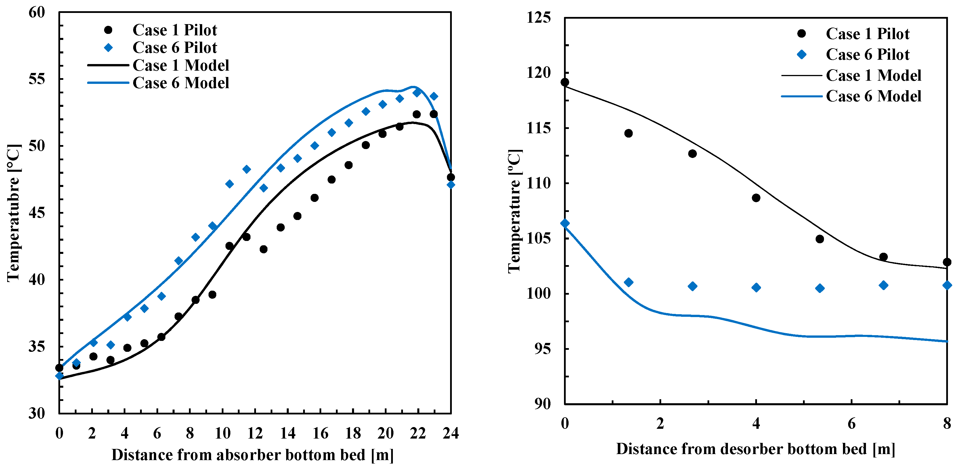
Figure 5.
(a) Main inputs to the plant for test with flue gas flow rate set-point reduction (kg/s). Rich solvent flow rate from absorber (kg/s) and reboiler duty (kW); (b) Pilot plant transient response and model output trajectory for CO2 product flow rate Fprod or CO2 desorbed (refer to FT3 in Figure 1); (c) Pilot plant transient response and model output trajectory for CO2 absorbed in absorber column, refer to Equation (11). The time t = 0 corresponds to the point from which the set point of flue gas volumetric flow rate was changed.

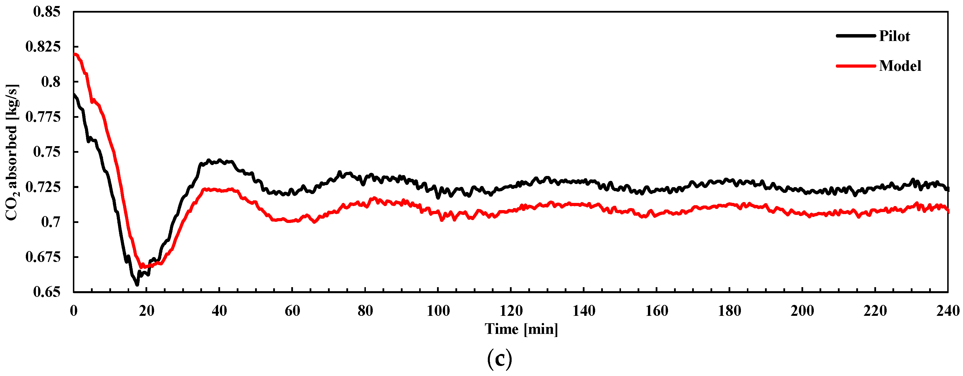
Figure 6.
(a) Main inputs to the plant for test with flue gas flow rate set-point increase (kg/s). Rich solvent flow rate from absorber (kg/s) and reboiler duty (kW); (b) Pilot plant transient response and model output trajectory for CO2 product flow rate Fprod or CO2 desorbed (refer to FT3 in Figure 1); (c) Pilot plant transient response and model output trajectory for CO2 absorbed in absorber column, refer to Equation (11). The time t = 0 corresponds to the point from which the set point of flue gas volumetric flow rate was changed.

Figure 7.
(a) Main inputs to the plant. Flue gas volumetric flow rate set-point change increase (kg/s). Rich solvent flow rate from absorber (kg/s) and steam flow to reboiler (kg/s); (b) Pilot plant transient response and model output trajectory for CO2 product flow rate Fprod or CO2 desorbed (refer to FT3 in Figure 1); (c) Pilot plant response in CO2 absorbed mass flow rate (kg/s). The time t = 0 corresponds to the point from which the set point of rich solvent flow rate was changed.


Figure 8.
Simulation results. Total stabilization times ts for open-loop ± 10% step changes in solvent flow rate and reboiler duty for the process variables (a) Lean CO2 loading Ll; (b) rich CO2 loading Lr; (c) CO2 absorbed CO2,abs and (d) CO2 desorbed CO2,des. Stabilization times are calculated for the response when the plant is operated at three different operating points in terms of flue gas mass flow rate, 100%, 80% and 60% of nominal capacity; refer to Table 5 and Table 6.
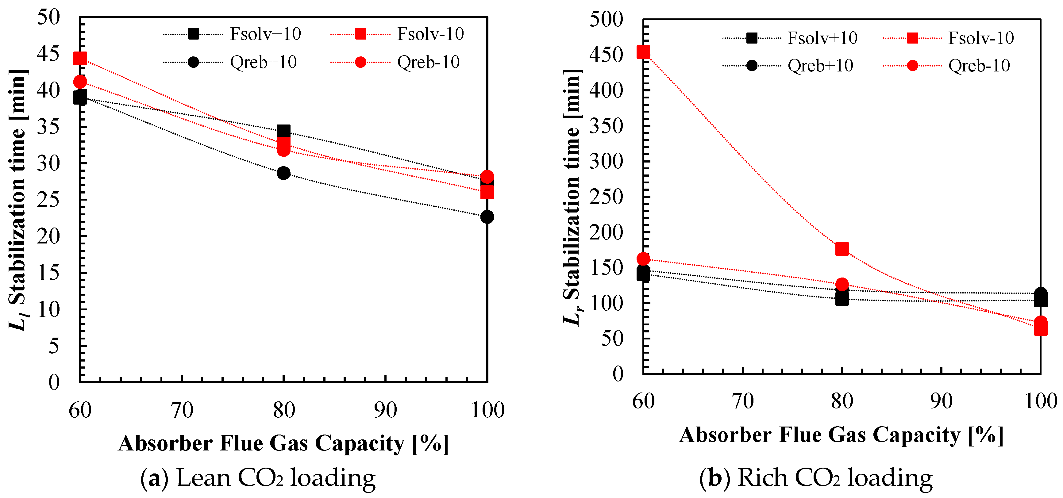

Figure 9.
Inputs to the pilot plant during simulations for load change ramp-down (Test 1) from 100 to 70% with a ramp rate of 10%/min reduction in flue gas flow rate, for control structures A, B, C and D. (a) Flue gas flow rate (kg/s), as a disturbance, and solvent flow rates (kg/s) of the rich pump as manipulated variables (MVs); (b) Reboiler duty (W) as MV. The red vertical dotted line shows when the transient event starts at t0.
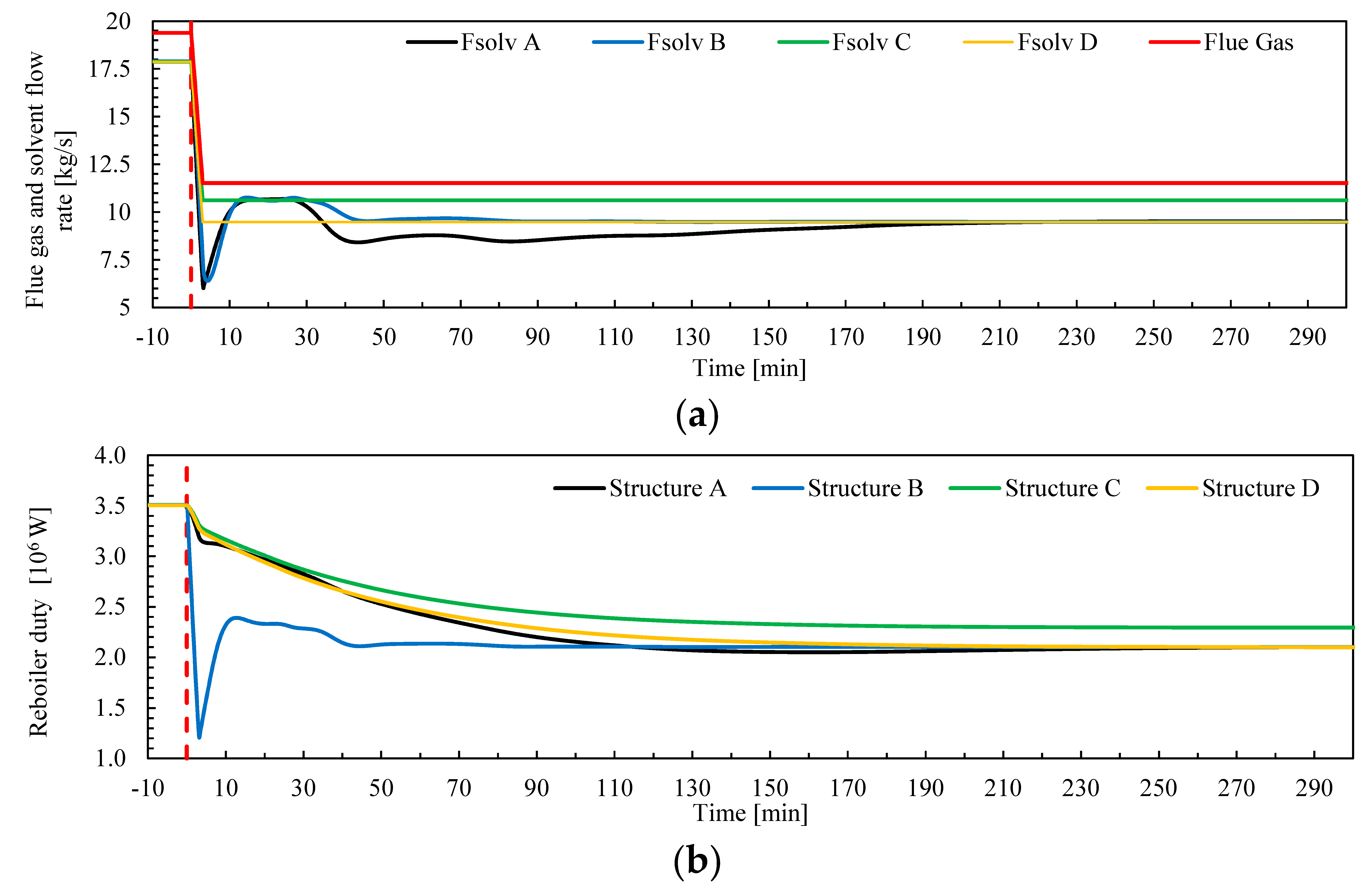
Figure 10.
Outputs from pilot plant model during simulations for load change ramp-down (Test 1) from 100 to 70% with a ramp rate of 10%/min reduction in flue gas flow rate, for control structures A, B, C and D. (a) CO2 capture ratio Cap, as controlled variable (CV); (b) CO2 desorption ratio Des; (c) CO2 absorption and desorption rates (kg/s). The red vertical dotted line shows when the transient event starts at t0.


Figure 11.
Outputs from pilot plant model during simulations for load change ramp-down (Test 1) from 100 to 70% with a ramp rate of 10%/min reduction in flue gas flow rate, for control structures A, B, C and D. (a) Lean CO2 loading at the inlet of the absorber; (b) Stripper bottom temperature as controlled variable (°C). The red vertical dotted line shows when the transient event starts at t0.

Figure 12.
Inputs to the pilot plant during simulations for load change ramp-up (Test 2) from 70 to 100% with a ramp rate of 10%/min increase in flue gas flow rate, for control structures A, B, C and D. (a) Flue gas flow rate (kg/s), as a disturbance, and solvent flow rates (kg/s) of the rich pump as manipulated variables (MVs); (b) Reboiler duty (W) as MV. The red vertical dotted line shows when the transient event starts at t0.

Figure 13.
Outputs from pilot plant model during simulations for load change ramp-up (Test 2) from 70 to 100% with a ramp rate of 10%/min increase in flue gas flow rate, for control structures A, B, C and D. (a) CO2 capture ratio Cap, as controlled variable (CV); (b) CO2 desorption ratio Des; (c) CO2 absorption and desorption rates (kg/s). The red vertical dotted line shows when the transient event starts at t0.


Figure 14.
Outputs from pilot plant model during simulations for load change ramp-up (Test 2) from 70 to 100% with a ramp rate of 10%/min increase in flue gas flow rate, for control structures A, B, C and D. (a) Lean CO2 loading at the inlet of the absorber; (b) Stripper bottom temperature as controlled variable (°C). The red vertical dotted line shows when the transient event starts at t0.
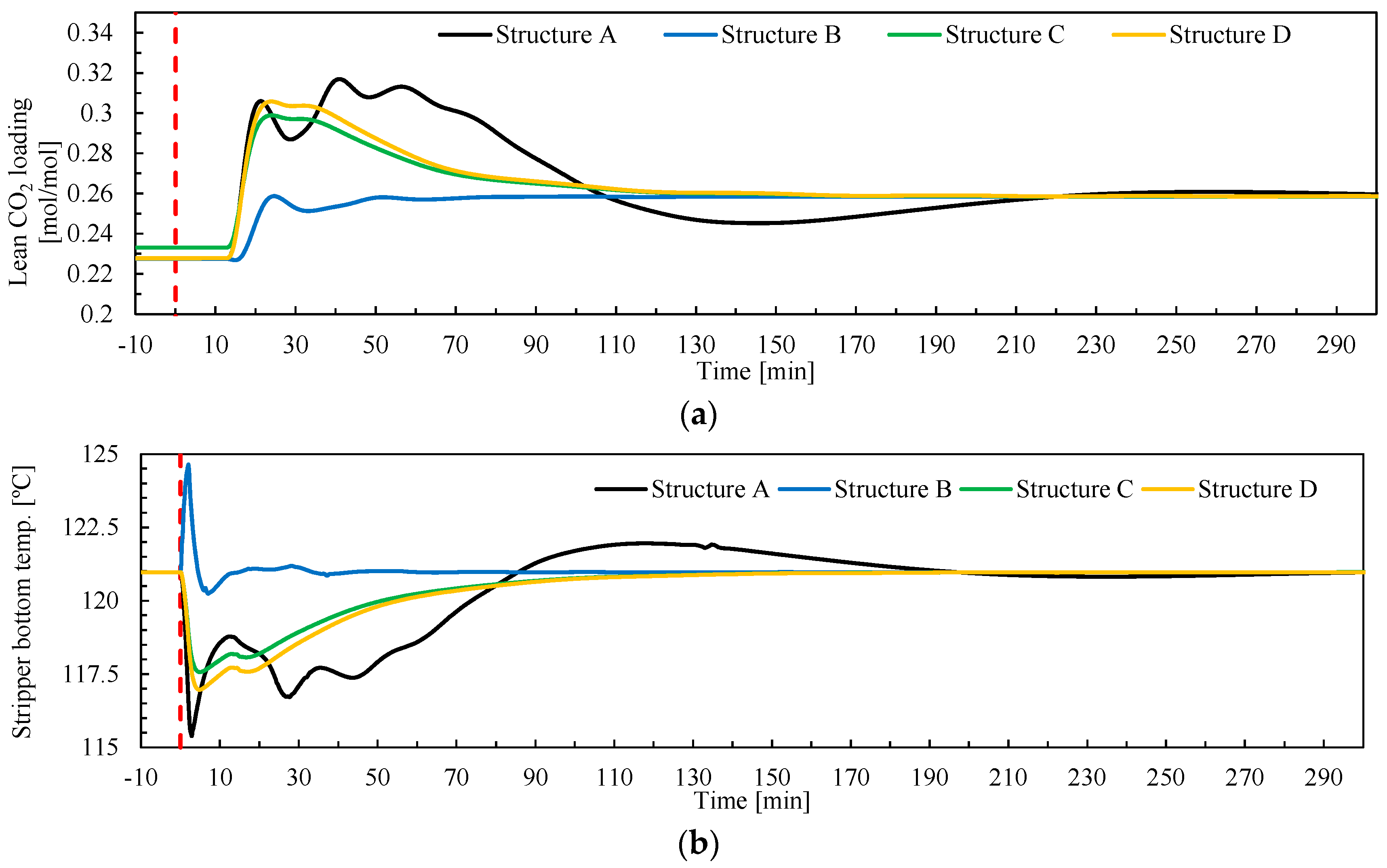
Table 1.
Size and materials of main process equipment at the amine plant at TCM DA with CHP stripper configuration.
Table 1.
Size and materials of main process equipment at the amine plant at TCM DA with CHP stripper configuration.
| Absorber | |
| Column cross sectional area (m2) | 3.55 × 2 |
| Column height (m) | 62 |
| Packing height (12 + 6 + 6) (m) | 24 |
| Water wash section height (3 + 3) (m) | 6 |
| Absorber packing type | Koch Glitsch Flexipac 2X |
| Absorber washer packing type | Koch Glitsch Flexipac 2Y HC |
| CHP Stripper | |
| Column cross sectional area (m2) | 1.33 |
| Diameter (m) | 1.3 |
| Packing height (m) | 8 |
| Water wash section height (m) | 1.6 |
| Absorber packing type | Koch Glitsch Flexipac 2X |
| Absorber washer packing type | Koch Glitsch Flexipac 2Y HC |
| Heat Exchanger L/Rich | |
| Duty (kW) | 10358 |
| Heat transfer area (m2) | 308 |
| Material | SS 316L |
| Reboiler | |
| Duty (kW) | 3365 |
| Heat transfer area (m2) | 142 |
| Material | SS 316L |
| Lean Amine Cooler | |
| Duty (kW) | 5182 |
| Heat transfer area (m2) | 78.8 |
| Material | TITANIUM |
Table 2.
Averaged values of total solvent inventory and its distribution within the main components of the TCM plant.
Table 2.
Averaged values of total solvent inventory and its distribution within the main components of the TCM plant.
| PCC Plant Main Components | Solvent Inventory (m3) |
|---|---|
| Absorber sump | 8.1 |
| Absorber packing | 8.4 |
| CHP stripper packing | 1.0 |
| CHP stripper sump | 2.3 |
| CHP reboiler | 0.4 |
| Cold rich solvent pipe | 2.2 |
| Cold lean solvent pipes | 5.2 |
| Hot rich solvent pipe | 1.1 |
| Hot lean solvent pipes (including reboiler pipes) | 8.2 |
| Lean/rich hx—lean side | 0.5 |
| Lean/rich hx—rich side | 0.5 |
| Lean cooler | 0.3 |
| TOTAL | 38.2 |
Table 3.
A selection of steady-state data cases obtained from the test campaign conducted at TCM plant during autumn 2015. The plant was operated with 30 wt. % aqueous MEA.
Table 3.
A selection of steady-state data cases obtained from the test campaign conducted at TCM plant during autumn 2015. The plant was operated with 30 wt. % aqueous MEA.
| Case | 1 | 2 | 3 | 4 | 5 | 6 | 7 | 8 | 9 | 10 |
|---|---|---|---|---|---|---|---|---|---|---|
| Gas flow rate (Sm3/h) | 59,461 | 59,468 | 59,442 | 59,499 | 59,544 | 46,973 | 46,973 | 46,973 | 46,973 | 46,973 |
| Rich solvent flow rate (kg/s) | 17.33 | 17.31 | 17.22 | 15.50 | 17.24 | 20.56 | 17.50 | 16.11 | 12.74 | 11.46 |
| L/G ratio (kg/kg) | 0.89 | 0.89 | 0.89 | 0.80 | 0.89 | 1.34 | 1.14 | 1.05 | 0.83 | 0.75 |
| Reboiler duty (kW) | 3417 | 3159 | 2664 | 2397 | 3056 | 2745 | 2669 | 2667 | 2659 | 2682 |
| Absorber inlet gas CO2 (vol%) | 3.64 | 3.61 | 3.59 | 3.58 | 3.59 | 3.60 | 3.62 | 3.62 | 3.62 | 3.62 |
| Absorber inlet gas O2 (vol%) | 15.52 | 15.54 | 15.55 | 15.46 | 15.35 | 15.30 | 15.48 | 15.49 | 15.51 | 15.52 |
| Absorber inlet gas H2O (vol%) | 3.98 | 3.92 | 3.93 | 4.01 | 4.22 | 3.80 | 3.36 | 3.46 | 3.52 | 3.43 |
| Absorber inlet gas N2 (vol%) | 79.09 | 79.02 | 78.85 | 78.57 | 78.20 | 78.18 | 78.88 | 78.94 | 79.06 | 78.96 |
| Loading rich (mol/mol) | 0.490 | 0.485 | 0.498 | 0.500 | 0.495 | 0.475 | 0.488 | 0.486 | 0.493 | 0.491 |
| Loading lean (mol/mol) | 0.280 | 0.294 | 0.333 | 0.341 | 0.314 | 0.342 | 0.329 | 0.310 | 0.260 | 0.229 |
| Stripper bottom temperature (°C) | 120.9 | 121.1 | 119.1 | 118.9 | 120.1 | 116.6 | 118.3 | 119.1 | 121.4 | 121.8 |
| CO2 product flow (kg/s) | 0.95 | 0.89 | 0.75 | 0.68 | 0.84 | 0.74 | 0.74 | 0.75 | 0.77 | 0.76 |
| CO2 capture rate (%) | 85 | 80 | 68 | - | 75 | 85 | 85 | 85 | 85 | 85 |
| Absorber packing height (m) | 24 | 18 | 18 | 18 | 18 | 24 | 24 | 24 | 24 | 24 |
Table 4.
Results from dynamic process simulation of the amine plant at TCM for the 10 steady-state operation cases. The pilot plant data for solvent CO2 lean loading (Ll), solvent CO2 rich loading (Lr), CO2 product flow rate (Fprod), specific reboiler duty (SRD) and stripper bottom temperature (Tstr) are shown. In addition, the model prediction during steady-state simulation for the same process variables is shown. Calculated absolute percentage errors (AP) and mean absolute percentage errors (MAP) between pilot plant measurements and simulated model predictions for the 10 steady-state operating cases are presented.
| Case | 1 | 2 | 3 | 4 | 5 | 6 | 7 | 8 | 9 | 10 | |
|---|---|---|---|---|---|---|---|---|---|---|---|
| Rich loading Lr (mol/mol) | Pilot plant | 0.489 | 0.485 | 0.498 | 0.500 | 0.495 | 0.475 | 0.488 | 0.486 | 0.493 | 0.491 |
| Model | 0.514 | 0.513 | 0.514 | 0.514 | 0.513 | 0.512 | 0.513 | 0.514 | 0.514 | 0.514 | |
| AP | 5.01 | 5.58 | 3.19 | 2.91 | 3.55 | 7.81 | 5.17 | 5.62 | 4.43 | 4.70 | |
| MAP | 4.80 | ||||||||||
| Lean loading Ll (mol/mol) | Pilot plant | 0.282 | 0.294 | 0.333 | 0.341 | 0.314 | 0.342 | 0.329 | 0.310 | 0.260 | 0.229 |
| Model | 0.257 | 0.273 | 0.309 | 0.306 | 0.279 | 0.343 | 0.312 | 0.292 | 0.241 | 0.224 | |
| AP | 8.93 | 7.24 | 7.16 | 10.06 | 11.34 | 0.35 | 4.98 | 5.94 | 7.10 | 2.35 | |
| MAP | 6.55 | ||||||||||
| CO2 Product flow Fprod (kg/sec) | Pilot plant | 0.95 | 0.89 | 0.75 | 0.68 | 0.84 | 0.74 | 0.74 | 0.75 | 0.77 | 0.76 |
| Model | 0.90 | 0.84 | 0.72 | 0.65 | 0.82 | 0.70 | 0.71 | 0.72 | 0.70 | 0.67 | |
| AP | 4.97 | 4.72 | 5.18 | 4.38 | 1.96 | 4.65 | 3.50 | 3.44 | 8.46 | 11.42 | |
| MAP | 5.27 | ||||||||||
| Specific reboiler duty SRD (kJ/kg) | Pilot plant | 3602 | 3562 | 3533 | 3509 | 3651 | 3727 | 3613 | 3561 | 3463 | 3538 |
| Model | 3791 | 3739 | 3726 | 3670 | 3724 | 3909 | 3744 | 3688 | 3783 | 3994 | |
| AP | 5.23 | 4.95 | 5.46 | 4.58 | 2.00 | 4.88 | 3.63 | 3.56 | 9.24 | 12.89 | |
| MAP | 5.64 | ||||||||||
| Stripper bottom temperature Tstr (°C) | Pilot plant | 120.9 | 121.1 | 119.1 | 118.9 | 120.1 | 116.6 | 118.3 | 119.1 | 121.4 | 121.8 |
| Model | 121.0 | 119.8 | 117.2 | 117.2 | 119.4 | 114.7 | 117.0 | 118.3 | 121.0 | 121.8 | |
| AP | 0.08 | 1.06 | 1.63 | 1.42 | 0.61 | 1.62 | 1.10 | 0.71 | 0.31 | 0.04 | |
| MAP | 0.86 |
Table 5.
Simulated pilot plant inputs’ set points for the three operating points to be studied, corresponding to 100%, 80% and 60% of flue gas mass flow rate capacity of the pilot plant. With Cap = 0.85 and Tstr = 120.9 °C for all cases.
Table 5.
Simulated pilot plant inputs’ set points for the three operating points to be studied, corresponding to 100%, 80% and 60% of flue gas mass flow rate capacity of the pilot plant. With Cap = 0.85 and Tstr = 120.9 °C for all cases.
| Pilot Load (%) | Fgas (kg/h) | Fsolv (kg/s) | (MW) |
|---|---|---|---|
| 100 | 19.3 | 17.6 | 3.5 |
| 80 | 15.3 | 13.2 | 2.7 |
| 60 | 11.6 | 9.5 | 2.1 |
Table 6.
Simulated pilot plant values for the process variables, lean CO2 loading Ll, rich CO2 loading Lr, CO2 capture ratio Cap and CO2 product flow rate, at three different operating points of the plant, corresponding to 100%, 80% and 60% of flue gas mass flow rate capacity of the pilot plant. With Cap = 0.85 and Tstr = 120.9 °C for all cases.
| Pilot Load (%) | Ll (mol/mol) | Lr (mol/mol) | Cap | Fprod (kg/s) |
|---|---|---|---|---|
| 100 | 0.280 | 0.501 | 0.85 | 0.91 |
| 80 | 0.246 | 0.514 | 0.85 | 0.72 |
| 60 | 0.228 | 0.514 | 0.85 | 0.55 |
Table 7.
Control structures for the supervisory control layer of the TCM amine plant. Key manipulated variables (MVs) are solvent flow rate Fsolv and reboiler duty Qreb. Controlled variables are CO2 capture ratio Cap to 85%, defined in Equation (12), and stripper bottom temperature Tstr to 120.9 °C. Control structure D controls Cap via a feed forward FF controller.
| Pairing 1 | Pairing 2 | |||
|---|---|---|---|---|
| Control Structure | Manipulated Variable | Controlled Variable | Manipulated Variable | Controlled Variable |
| A | Fsolv | Cap | Qreb | Tstr |
| B | Qreb | Cap | Fsolv | Tstr |
| C | Fsolv | L/G | Qreb | Tstr |
| D | Fsolv | Cap, with FF | Qreb | Tstr |
Table 8.
Total stabilization times of the floating process variables for the different control structures, when ramping down the plant tt,down from 100% flue gas mass flow rate to 70%; and when ramping up the plant tt,up from 70% flue gas mass flow rate to 100%.
Table 8.
Total stabilization times of the floating process variables for the different control structures, when ramping down the plant tt,down from 100% flue gas mass flow rate to 70%; and when ramping up the plant tt,up from 70% flue gas mass flow rate to 100%.
| Control Structure | Process Variable | tt,down (min) | tt,up (min) |
|---|---|---|---|
| A | CO2 Absorbed | 3.3 | 71.0 |
| CO2 Desorbed | 36.3 | 112.7 | |
| Ll | 187.7 | 201.0 | |
| B | CO2 Absorbed | 4.0 | 5.2 |
| CO2 Desorbed | 35.3 | 27.5 | |
| Ll | 68.2 | 46.7 | |
| C | CO2 Absorbed | 3.6 | 97.7 |
| CO2 Desorbed | 56.5 | 63.7 | |
| Ll | 172.2 | 115.5 | |
| D | CO2 Absorbed | 6.2 | 96.8 |
| CO2 Desorbed | 50.3 | 59.2 | |
| Ll | 185.0 | 113.8 |
Table 9.
Simulation results for accumulated reboiler energy consumption Qreb (MJ), accumulated CO2 emitted CO2,em and accumulated CO2 captured CO2,cap during the transient event (8 h) for the different control structures A,B, C and D (refer to Table 7), when ramping up and down the plant (between 100% and 70% of flue gas mass flow rate). Static plant refers to an ideal static plant that changes from the initial operating conditions to the final operating conditions instantaneously at time t = 0. An integration time of tf = 480 min was utilized to calculate the values for the ideal static plant.
| Transient event | Indicator | Static Plant | A | B | C | D |
|---|---|---|---|---|---|---|
| Ramp down | Qreb (MJ) | 60,441 | 63,353 | 60,926 | 69,045 | 64,046 |
| CO2,em (tons) | 2.66 | 2.64 | 2.65 | 0.96 | 2.39 | |
| CO2,cap (tons) | 15.70 | 15.76 | 15.75 | 17.44 | 16.01 | |
| Ramp up | Qreb (MJ) | 100,924 | 100,898 | 100,655 | 98,973 | 98,667 |
| CO2,em (tons) | 4.49 | 4.51 | 4.53 | 4.77 | 4.94 | |
| CO2,cap (tons) | 26.41 | 26.39 | 26.37 | 26.13 | 25.96 |
© 2017 by the authors. Licensee MDPI, Basel, Switzerland. This article is an open access article distributed under the terms and conditions of the Creative Commons Attribution (CC BY) license (http://creativecommons.org/licenses/by/4.0/).
Share and Cite
MDPI and ACS Style
Montañés, R.M.; Flø, N.E.; Nord, L.O. Dynamic Process Model Validation and Control of the Amine Plant at CO2 Technology Centre Mongstad. Energies 2017, 10, 1527. https://doi.org/10.3390/en10101527
AMA Style
Montañés RM, Flø NE, Nord LO. Dynamic Process Model Validation and Control of the Amine Plant at CO2 Technology Centre Mongstad. Energies. 2017; 10(10):1527. https://doi.org/10.3390/en10101527
Chicago/Turabian StyleMontañés, Rubén M., Nina E. Flø, and Lars O. Nord. 2017. "Dynamic Process Model Validation and Control of the Amine Plant at CO2 Technology Centre Mongstad" Energies 10, no. 10: 1527. https://doi.org/10.3390/en10101527
Note that from the first issue of 2016, this journal uses article numbers instead of page numbers. See further details here.