1. Introduction
In recent years multilevel converters have been developed extensively due to industry demands. The achieved advances in terms of efficiency and power quality have made them more attractive for the industry [
1]. Multilevel converters have several advantages compared with the classical topologies based on two or three level voltage source converters (VSCs). These advantages are e.g., low harmonic distortion or reduced switching frequency [
2]. The most common topologies which are widely used in industrial applications are the cascaded H-bridge (CHB) and the neutral-point-clamped (NPC). However, these topologies have several limitations such as the bulky transformer required by the CHB or the limited number of levels available in the NPC [
3,
4].
As a solution to these limitations, the modular multilevel converter (MMC) topology was developed. The MMC was originally designed to be used in high-voltage direct current (HVDC) transmission lines [
5]. However, in recent years, MMC has been an emerging topology used in medium-voltage (MV) applications such as in flexible AC transmission systems (FACTS) or medium-voltage drives (MVDs) [
6,
7].
The MMC can be adapted to a wide range of voltages/power by modifying the number of series-connected submodules. In high-voltage applications the MMC can be directly connected, avoiding the use of transformers and reducing the overall cost. Additionally, due to their modularity, the switching frequency can be considerably reduced without worsening the power quality.
The MMC topology presents however several disadvantages which reduce its performance. One of them is the capacitor voltage unbalance which appears due to the current that flows through the submodules [
8,
9]. Another disadvantage is the circulating current. This is the result of a mismatch between the output voltage of different phase arms and the input direct-current (DC) voltage [
10].
There are several studies in the literature where the circulating current has been studied. In [
5], the circulating current model is obtained from the energy stored in the capacitors. However, in [
10] a more accurate study related with the circulating current has been carried out. In this study, the analytical expressions of the currents and voltages have been shown.
The circulating current generates several undesirable effects which reduce the efficiency and the performance, such as higher capacitor voltage ripple and higher power losses [
11]. Thus, a circulating current controller is the best option to reduce the amplitude of this current.
Yang et al. [
12] proposed a proportional integrator (PI)-based controller to reduce the circulating current. The control method proposed is based on transforming the frames from an
a-c-b sequence into a
dq sequence. However, this method has the disadvantage of any synchronization problem reduces the effectiveness of the control. In addition, simulation results are provided.
Tu et al. [
13] proposed a proportional resonant (PR) controller to control the circulating current under unbalanced voltages. Under unbalanced voltages, the circulating current is composed of positive-sequence, negative-sequence and zero-sequence, however, only the double-line-frequency is controlled. Moreover, the proposed controller was only validated by simulation results. A PR controller was also used in [
14], but in this case, the PR controller was modified for better digital realization and noise injection and more harmonics were controlled.
In [
15] a plug-in repetitive controller to reduce the circulating current was proposed. However, both simulation results and experimental results were carried out in a single-phase MMC, so the results cannot be validated for a three-phase MMC since the behavior is not the same.
In this paper two approaches to reduce the circulating current and thus the power losses are proposed. The circulating current controllers proposed are based on an αβ-frame. The use of an αβ-frame avoids the synchronization problems and reduces the control complexity [
16]. The first approach presented in this paper is based on parallel-connected PR controllers tuning to the frequencies presented in the circulating current.
The second approach is based in a digital plug-in repetitive controller. The proposed repetitive controller has the advantage of a simple structure and good harmonic suppression [
17]. In this paper, these two algorithms to track harmonics will be compared, similar to [
18], but focusing on the reduction of the circulating current fundamentally due to the use of the proposed algorithm to eliminate this current, which is a relevant contribution with respect to previous work.
In addition, due to the fact that it is difficult to find in the literature studies where the proposed controllers are tuned to reduce the circulating current, in this paper, the authors propose tuning techniques for both dq-frame-based controllers and αβ-frame-based controllers in order to reduce the circulating current. This article aims to provide several guidelines to choose, design and tune circulating current controllers.
Moreover, a stationary frame saturator has been proposed in order to limit the output voltage reference. The output voltage saturator in MMCs is a key issue that has not been well studied in the technical literature and greatly affects the performance of the controllers. This paper is organized as follows:
Section 2 presents the MMC topology and the circulating current is fully analyzed.
Section 3 presents the
dq-frame based controllers where are explained and tuned. The proposed controllers, both resonant controllers and the repetitive controller are analyzed in detail in
Section 4. Finally,
Section 5 shows the experimental results. In addition to the experimental results, both the processing platform and a prototype are described. This paper’s conclusions are summarized in
Section 6.
2. Modular Multilevel Converter
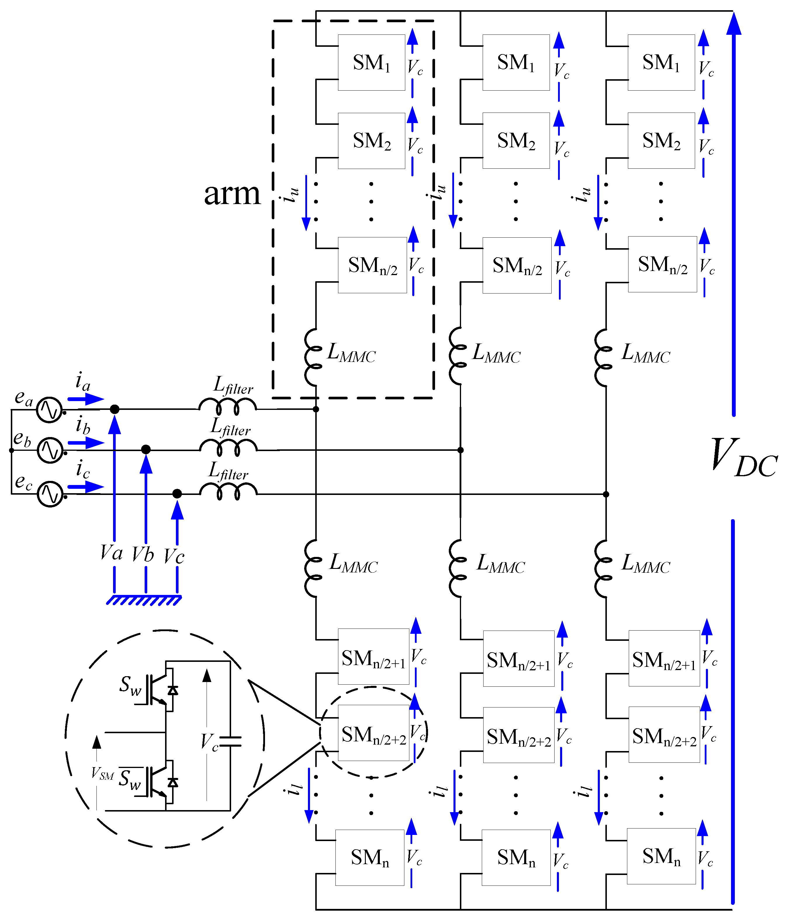
Figure 1 shows the structure of a three phase MMC, which is composed of six arms. Each arm consists of
n/2 series-connected submodules (SMs), where
n is the number of SM per phase, and an arm inductor
LMMC. The submodule is a half H-bridge that contains two insulated-gate bipolar transistors (IGBTs), two reversing diodes and a DC storage capacitor. The two switches (
and
) in each SM are controlled with complementary signals, resulting in two active switching states that can connect or bypass the respective capacitors to the converter leg. Consequently, the output voltage
VSM (
Figure 1) can be determined based on the switching states. When
is switched ON,
is switched OFF. Here, the output voltage is
Vc. In contrast, when
is switched OFF,
is switched ON, and the output voltage is zero.
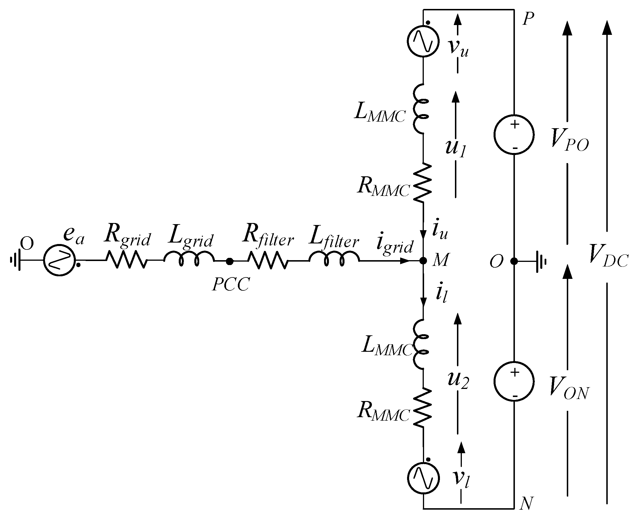
The mathematical model of the power converter is essential since it allows one to know the behavior and performance of the converter. The MMC mathematical model is calculated using the MMC structure shown in
Figure 2, which is a simplification of the structure shown in
Figure 1. It shows one phase of the MMC connected to the grid across an inductor filter.
The SM can be modeled as an alternative current (AC) power supply thus, the generated voltage in the upper arm is and the generated voltage in the lower arm is . The DC-bus can be also modeled as two DC power supplies connected in series with the common point connected to ground.
Ideally the current that flows through the arms,
which is the current that flows through the upper arm and
which is the lower arm, are the sum of a DC component and an AC component of the fundamental frequency. However, due to the AC current flow through the SM capacitors, the capacitor voltages vary with time. As result, there is a voltage difference between DC-bus voltage and each arm voltage, which leads to a problem of circulating currents in each arm [
13].
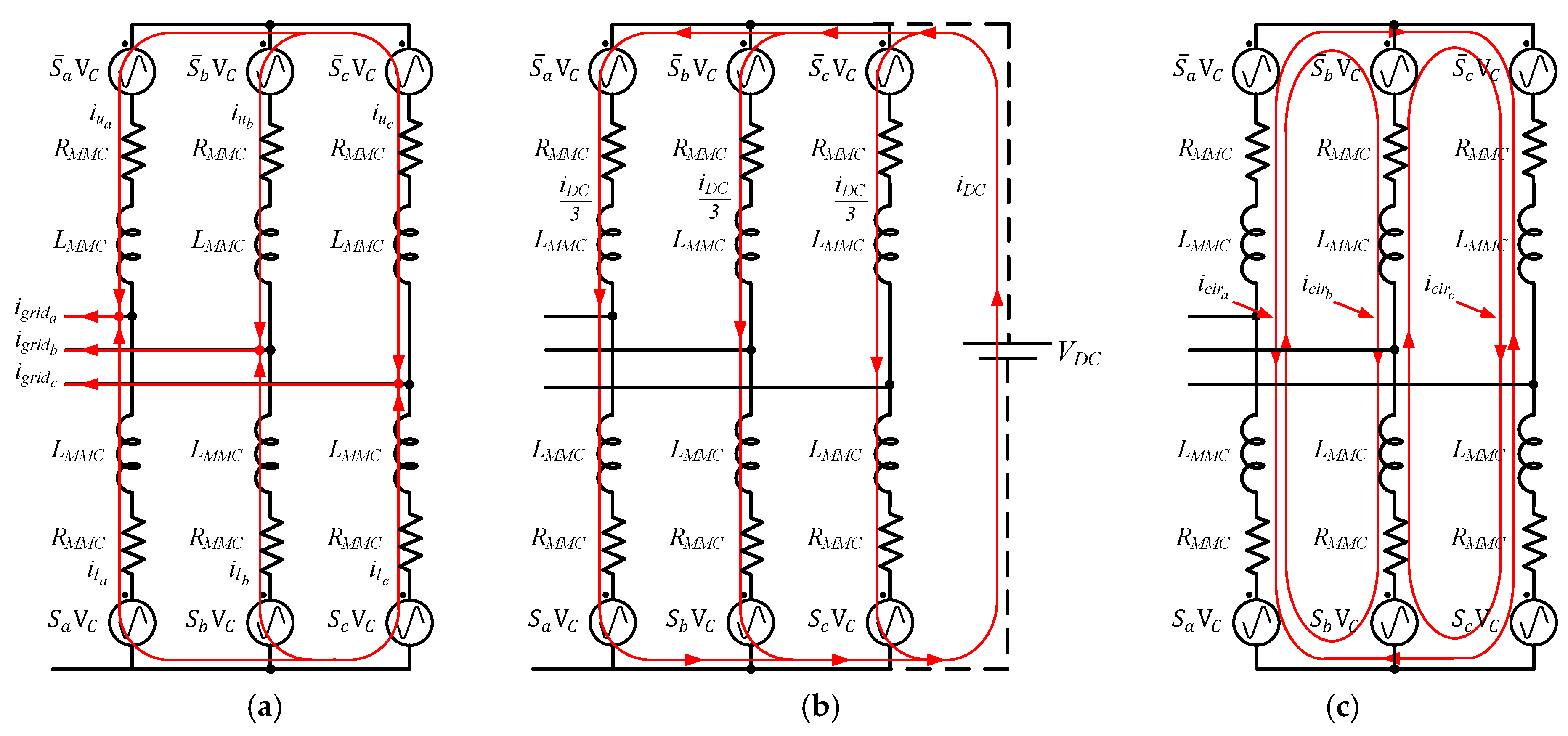
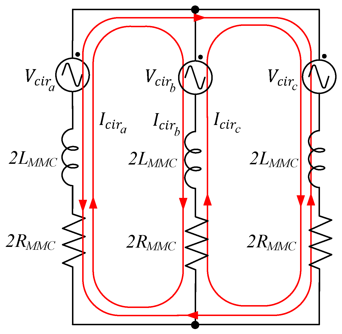
Figure 3 shows the abovementioned existing currents in the MMC. As demonstrated in the figure, each current has different paths. Therefore, the value of
and
are given by (1) and (2), respectively:
From (1) and (2) it is obtained that the circulating current
is given by:
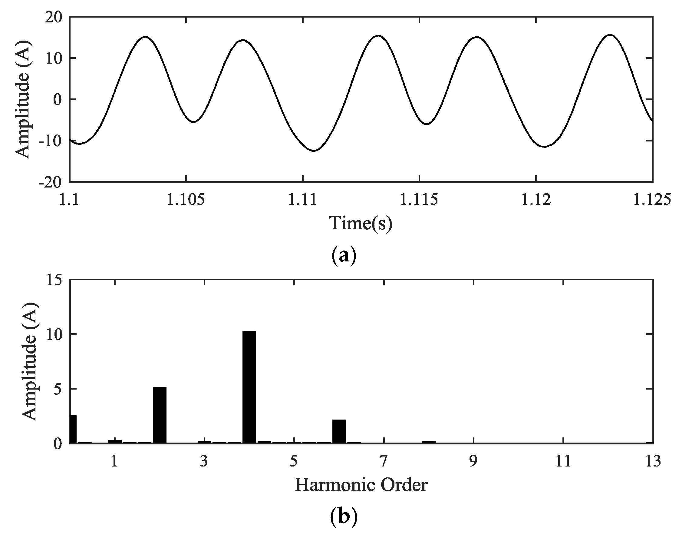
The circulating current is in negative sequence and is composed of several harmonics as demonstrated previously [
8]. The harmonics present in the circulating current are the second-order harmonic, fourth-order, sixth-order and eight-order harmonic as shown in
Figure 4. Thus, the circulating current can be expressed as the sum of multiple harmonics and a DC component (see Equation (4)):
The amplitude and the phase of each component are analyzed in detail in [
10]. The circulating current model shown in
Figure 3c can be simplified as shows
Figure 5. The circulating current generates several undesirable effects which reduce the efficiency and the performance. Some of these effects are listed below:
Capacitor voltage ripple: the circulating current increases the voltage ripple since it depends on the amplitude of the arm currents.
Power losses: The circulating current increases the arm currents and thus, the power dissipated by RMMC is higher. Moreover, the power losses in the switching devices are also increased.
Inductor saturation: As in the previous case, the amplitude of the arm current is affected by the circulating current. Therefore, if the circulating current is high, the inductor LMMC can be saturated in the case of ferromagnetic core inductors.
Power quality: As demonstrated above, the circulating current is composed of several harmonics which reduce the quality of the power exchanged with the grid. Moreover, the reactive power exchanged greatly increases its value. These energy consumptions, reduce the performance of the controllers as well as the capability of the MMC. This fact is critical if the MMC is intended to be used in FACTS applications where the voltage support or reactive power compensation is intended to be used.
The circulating current can be minimized by increasing the SM capacitors or increasing the inductors. Nevertheless, the cost of the capacitors has to be taken into account. In addition, the size of the inductors has an impact in the MMC performance increasing the losses. Thus, a circulating current controller is the best option to reduce the amplitude of this current.
The three differential equations which describe the behavior of the circulating current can be obtained from
Figure 2 and
Figure 5 and are the following:
Equations (5) can be transformed into the αβ-frame as follows:
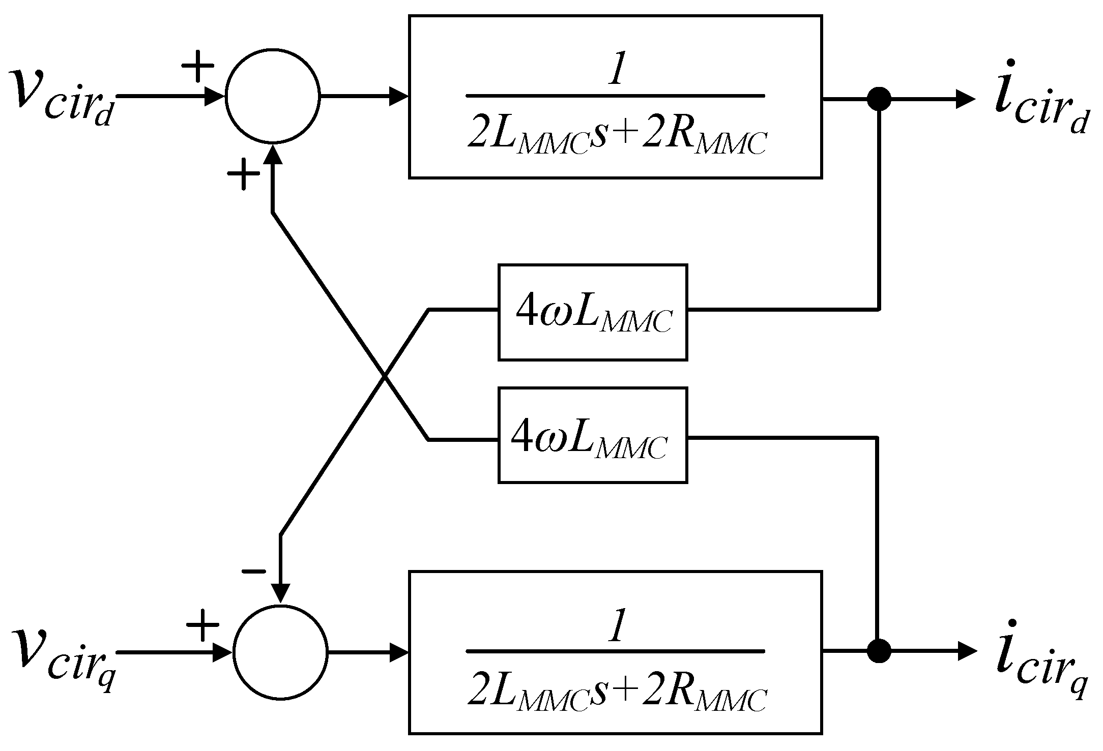
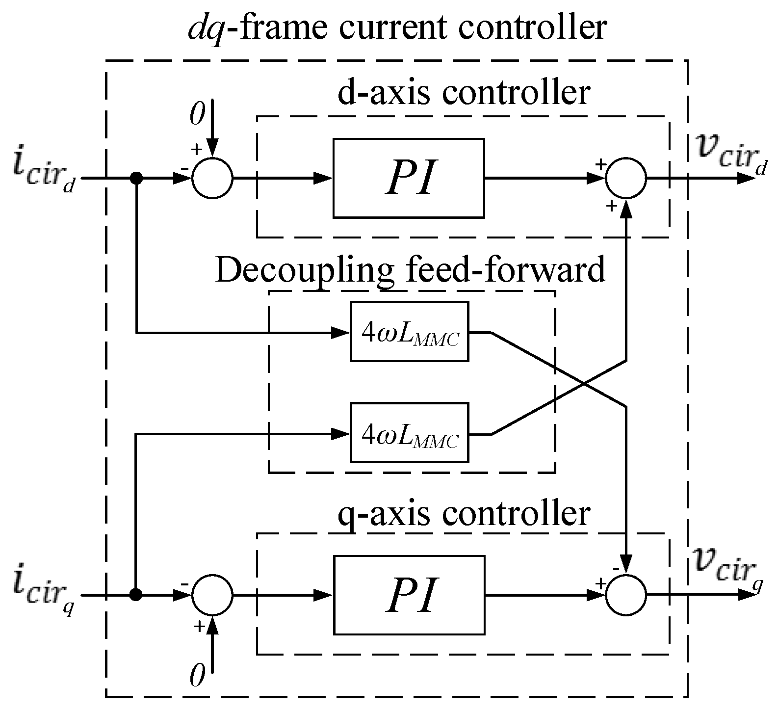
Assuming steady-state operation condition, Equations (6) are then transformed to the dq-frame:
Equations (7) demonstrate that there is a cross coupling between
and
. This cross coupling increases the control complexity. The circulating current obtained in shown in
Figure 6.
In order to eliminate this coupling a decoupling feed-forward with gain
is used. Then, the transfer function of the circulating current is given by:
In order to control the circulating current, the model must be discretized. The plant shown in (8) is discretized using zero-order hold (ZOH) discretization technique. The discretized model obtained is:
Depending on the frame used, αβ-frame or dq-frame different control strategies are adopted.
4. αβ-Frame Controller
As described in
Section 2, the circulating current is composed of even order harmonics. This means that in order to reduce it value, if the
dq-frame transformation is used, a different phase from the grid must be used. The use of
dq-frame based controllers presents several problems. One of them is the phase estimation since there is no guarantee that the circulating current phase is in phase with the grid voltage. Moreover, the circulating current is composed of
n-harmonics, however in the literature this n-harmonics are neglected and the double-frequency harmonic is only considered. This simplification is not valid under grids with voltage unbalances and harmonics.
In this paper the use of circulating current controllers in the αβ-frame is proposed. The use of an αβ-frame instead of a dq-frame presents the advantage that the circulating current phase does not need to be determined. Two approaches to reduce the circulating current are presented in this paper. The first approach is based on the use of a resonant controllers. The second approach consist of reducing the circulating current by means of a repetitive controller.
4.1. Resonant Controllers
In order to control the circulating current, a resonant controller (RC) has been chosen since theoretically it achieves an infinite gain at the frequency of interest. This frequency is also called resonant frequency
. Since a resonant controller presents an infinitive gain at the frequencies
, it is able to track or reject a sinusoidal signal of frequency
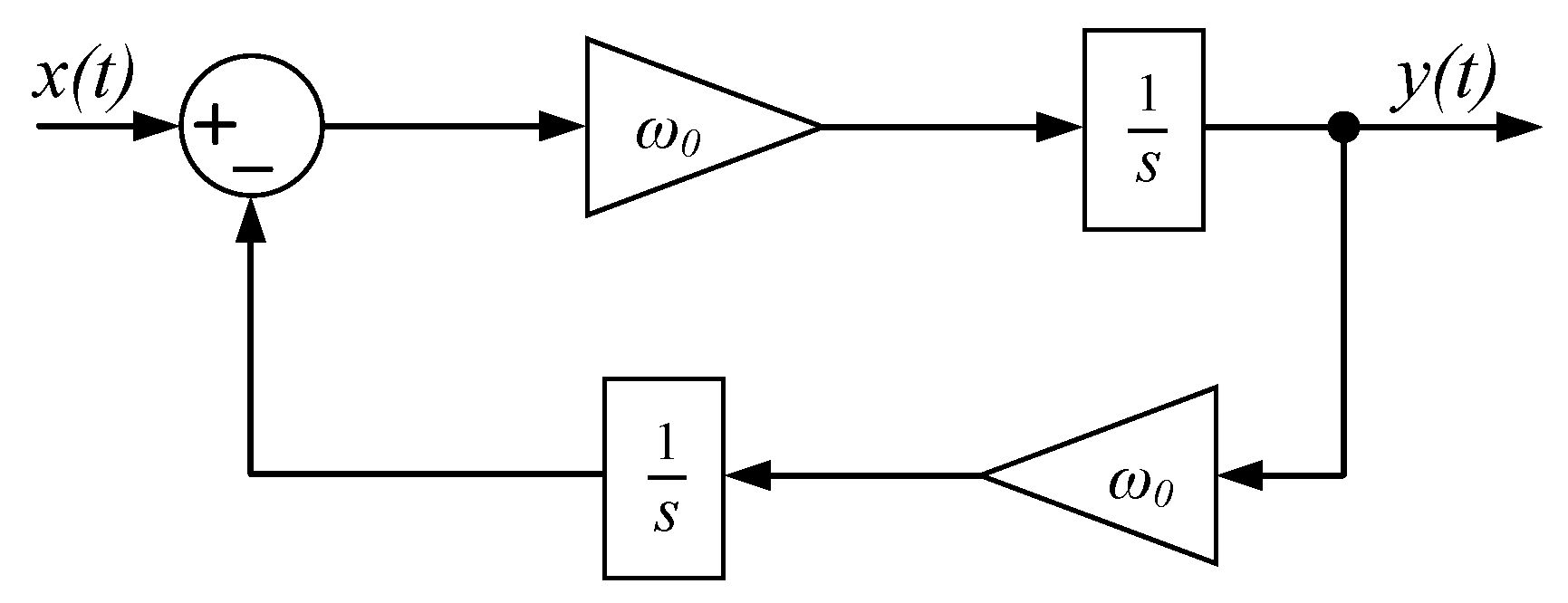
with zero steady-state error. In this paper the second order generalized integrator (SOGI) has been chosen as resonant controller [
18]. The transfer function of the SOGI is shown in (13) and its continuous time block diagram is represented in
Figure 8 where
x(
t) is the input signal and
y(
t) is the output signal.
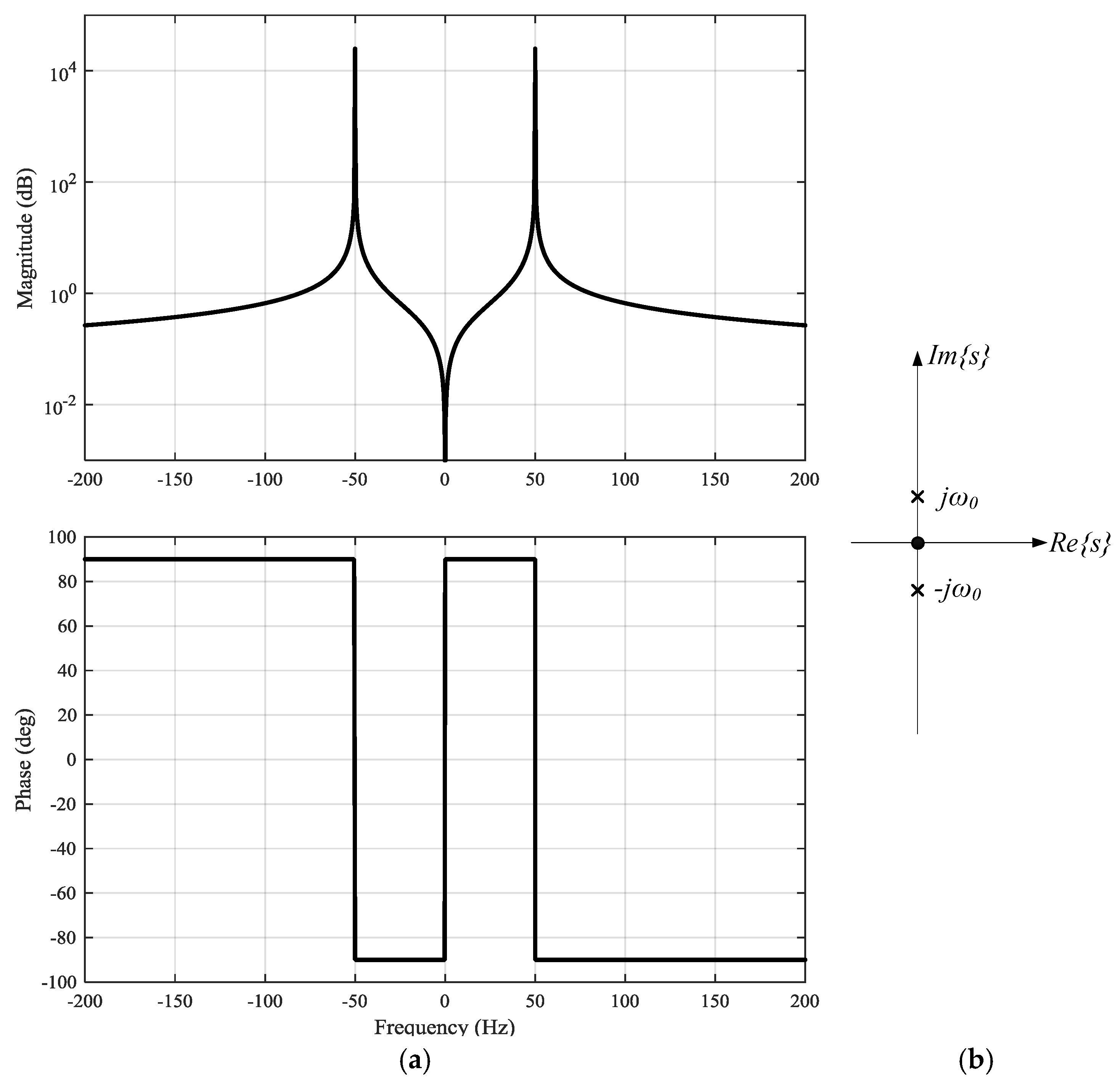
This controller has infinite gain and no phase control at the resonant frequency. The Bode diagram is shown in
Figure 9a and the zero-pole map is shown in
Figure 9b. It has an excellent selectivity but the addition of several SOGIs in parallel may endanger the system stability.
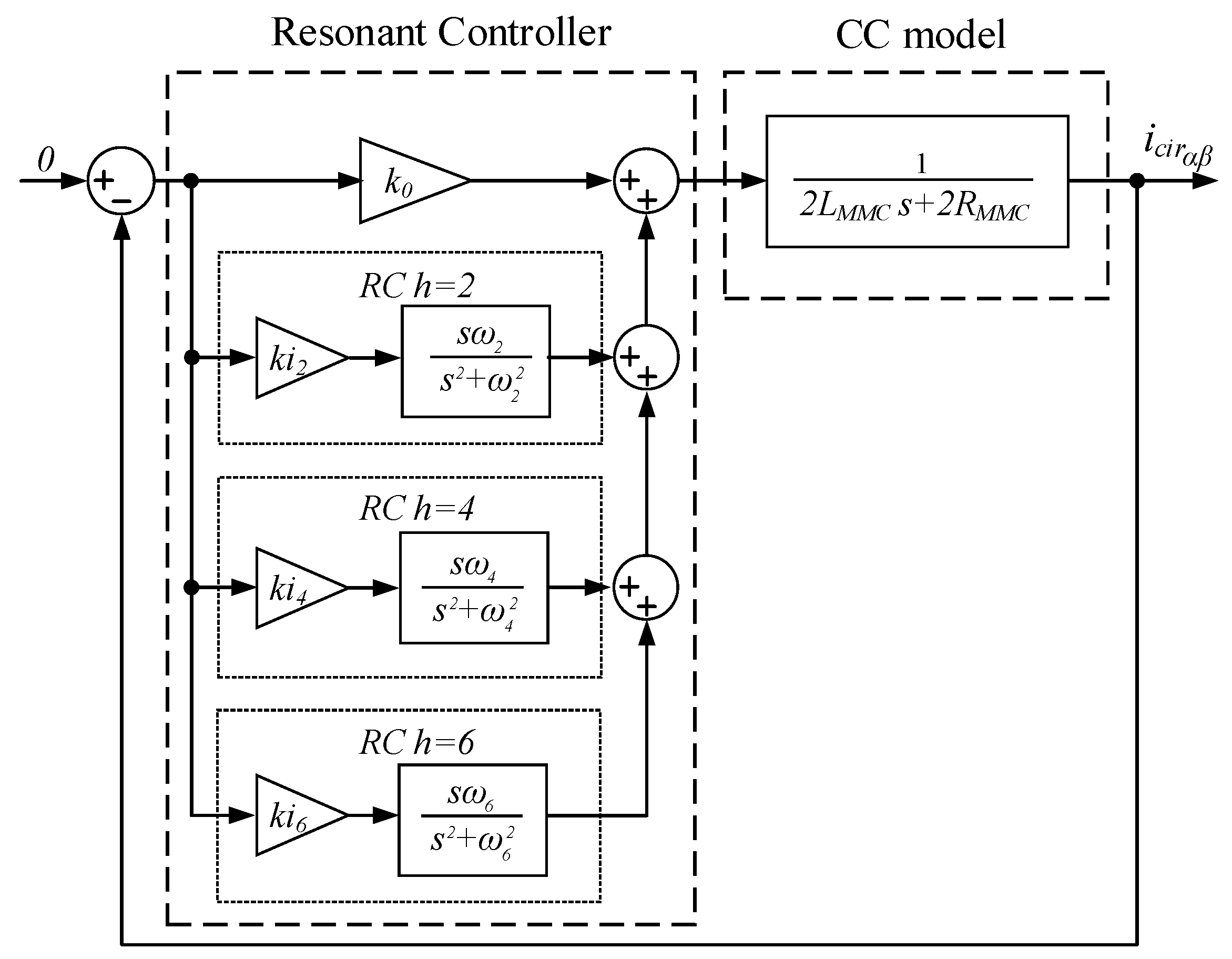
As demonstrated in
Figure 4b, the circulating current is mainly composed of three harmonics. Hence, three resonant controllers are used. The RCs are tuned to control the second (
h = 2), the fourth (
h = 4) and the sixth harmonic (
h = 6). The control scheme proposed is shown in
Figure 10. The proposed configuration ensures that all the harmonics presented in the circulating current are eliminated. The Bode diagram of the proposed controller is shown in
Figure 11. The figure illustrates that controller has only high gain at the selected resonant frequencies (
h = 2,
h = 4 and
h = 6).
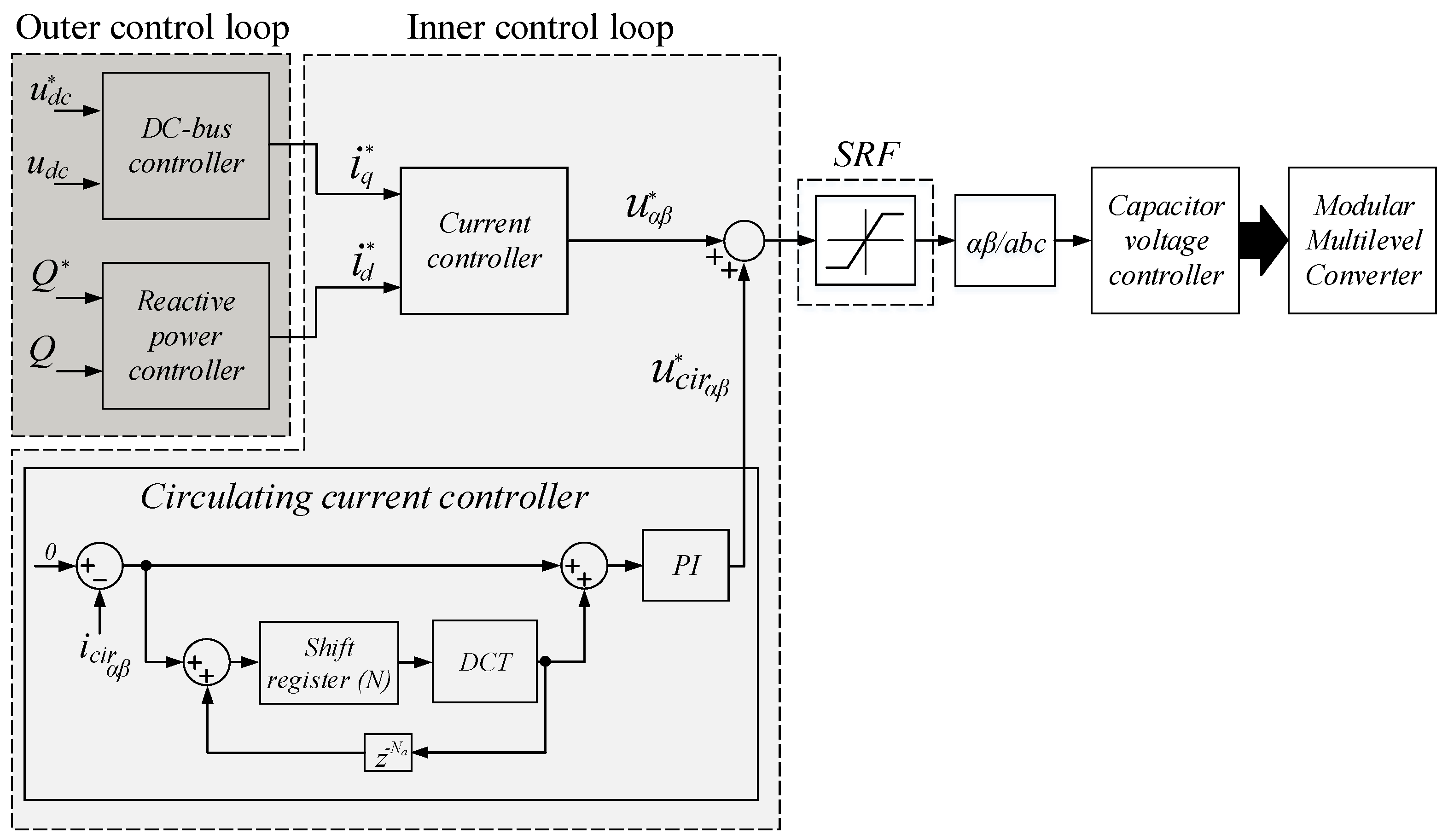
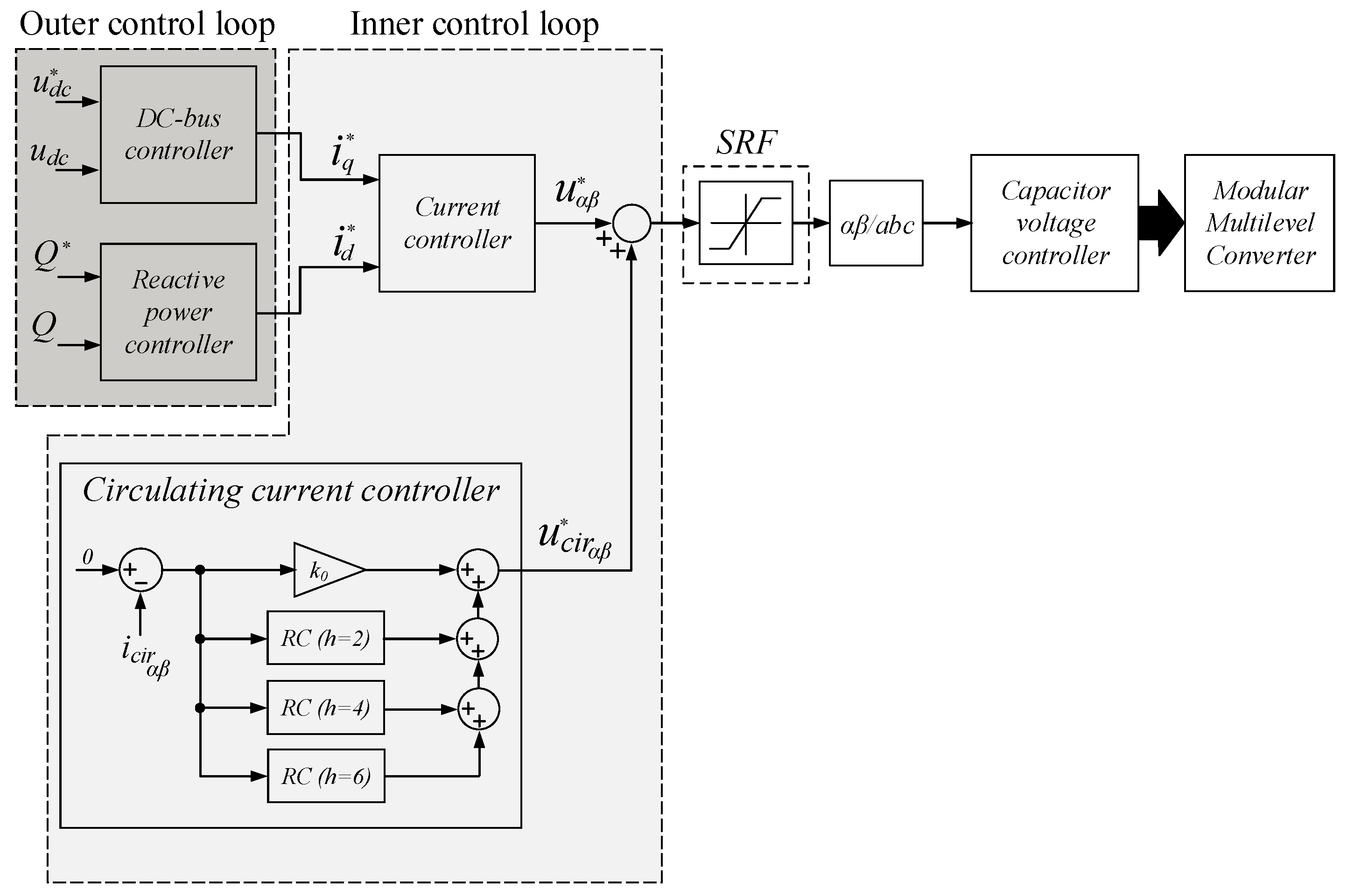
The proposed overall control scheme is shown in
Figure 12. The control scheme has been divided into two control loops: the outer control loop and the inner control loop. The outer control loop is composed by the DC-bus voltage controller and the reactive power controller. The output outer control loop is the
and
reference currents. The inner control loop is composed by the circulating current controller and the current controller. The inner control loop is the responsible to generate the output voltage reference. In the approach presented in this paper, both current controller output
and circulating current controller output
are added in αβ-frame. Finally, a stationary-frame saturator is used to limit the reference. The use of a saturator is an important key which are analyzed in detail below.
The SOGI is digitally implemented using the difference equation of the controller. Thus, a discretization technique must be used. There are several discretization techniques that can be used. The most common discretization techniques are Forward Euler, Backward Euler, Tustin, or Zero-Order Hold. In this paper the discretization technique used is Tustin with prewarping (TPW) since it has low resonant frequency deviation [
18]. The correspondence between the s-plane and the z-plane using TPW is shown in Equation (14):
Applying (14) in (13) the SOGI discrete model is obtained:
If Equation (15) is decomposed in difference equation, the following expression is obtained:
Each RC block in
Figure 10 is replaced with a block that implements Equation (16) plus an integral gain
. In parallel with the RC controllers a proportional gain
is used in order to decrease the settling time. The tuning of each RC is described by Equation (17), where
,
.
is the sampling period used by the controller,
is the harmonic order (in this paper it is supposed
and
),
,
,
is the natural pulsation and
is the damping factor, typically chosen as
:
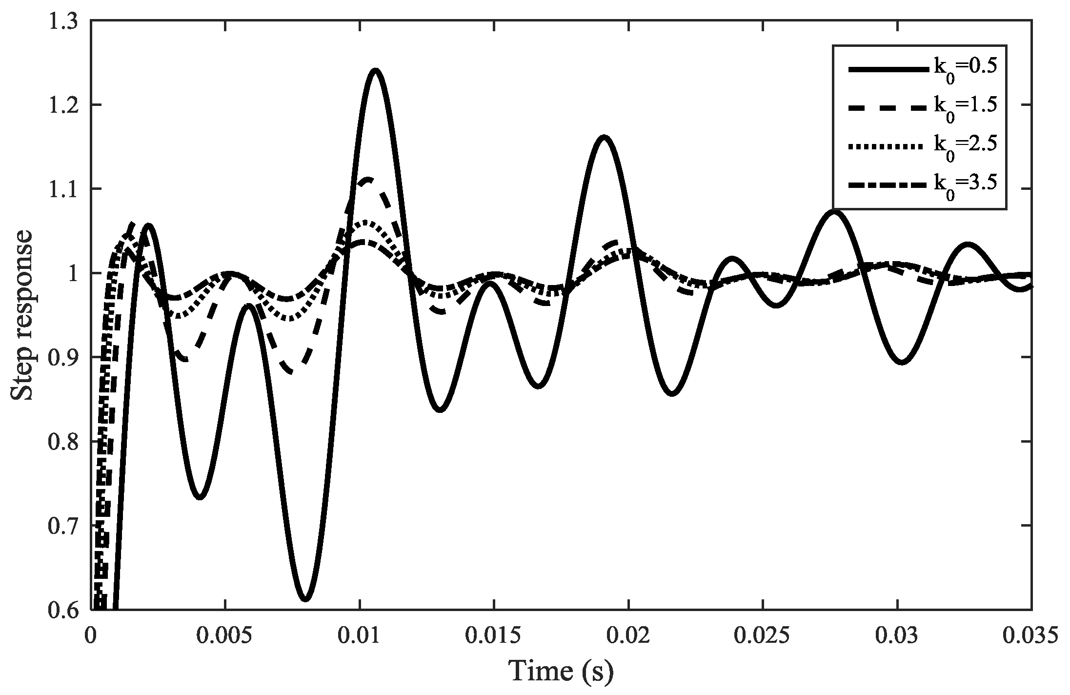
The gain
used to reduce the settling time should be enough high in order to increase the stability and reduce the oscillations.
Figure 13 shows the step response of the RC controller for different
values.
4.2. Repetitive Controllers
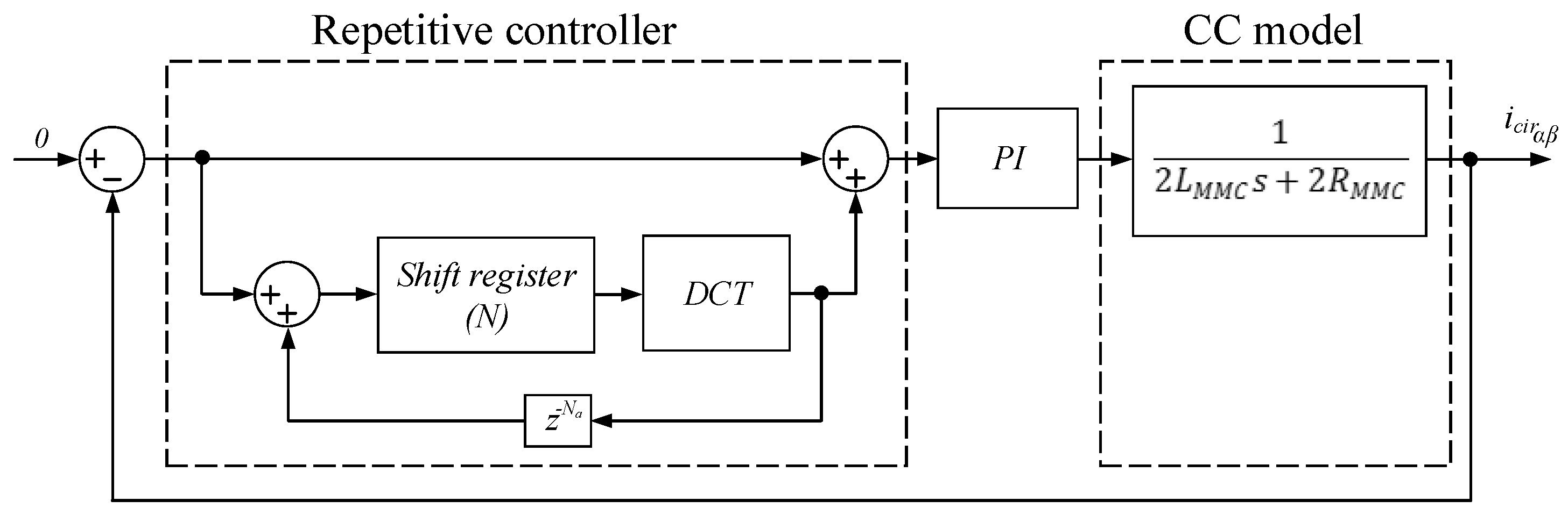
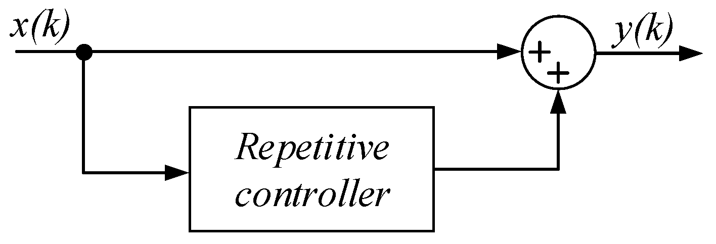
The repetitive controller emulates a bank of PR filters, introducing only gain peaks at the frequencies of interest. The advantage of this control scheme is that there is no need to repeat the control structure for each harmonic. Thus, only one control loop is needed in order to compensate all the harmonics. This controller can eliminate harmonics of the input signal up to the Nyquist frequency. The scheme of a plug-in repetitive controller is shown in
Figure 14.
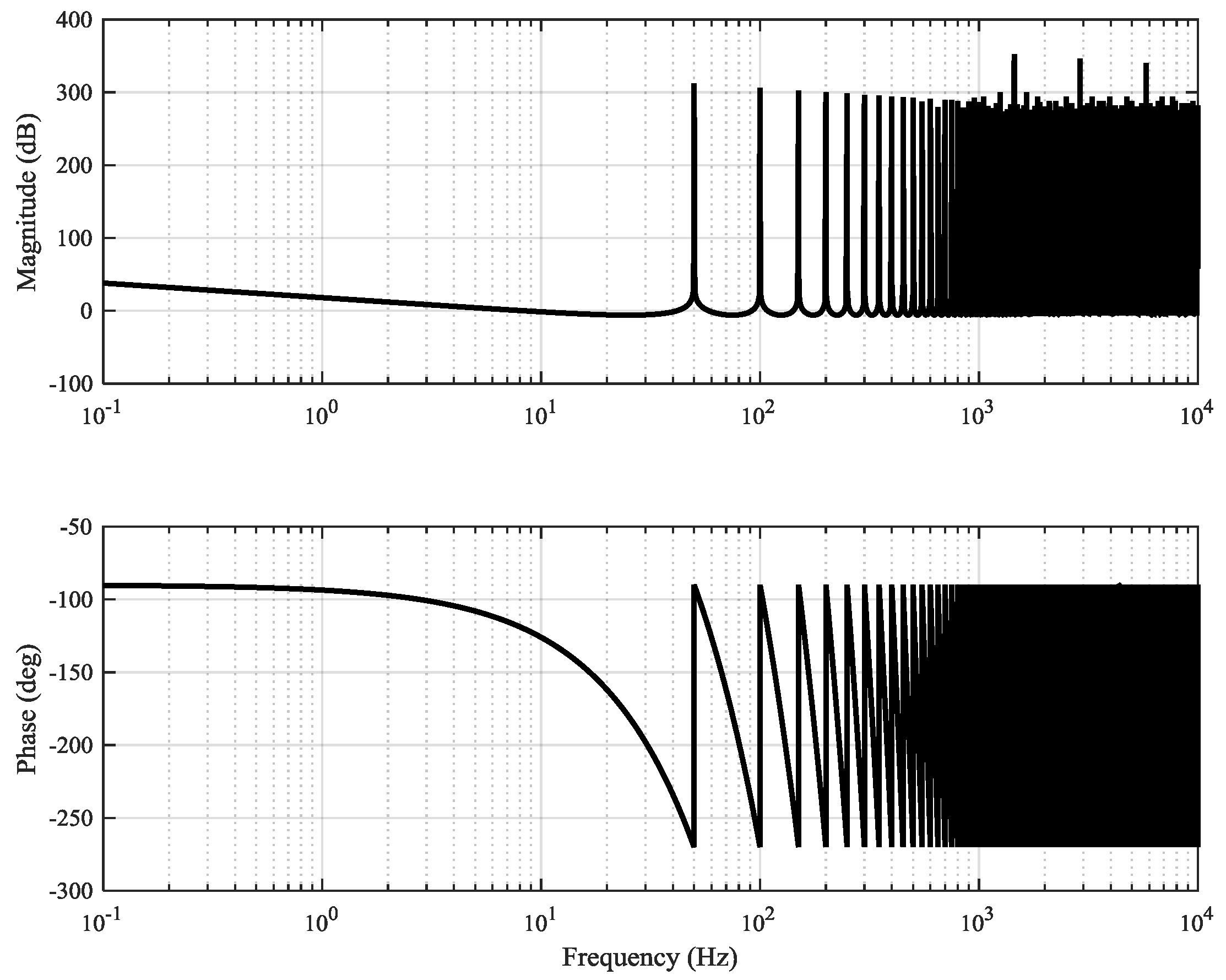
The repetitive loop has an infinite gain to all frequencies that are multiples of
1⁄T Hz, where
T is the period of the fundamental signal (
Figure 15). This ensures disturbance rejection and zero steady-state error for signals with spectral content at these frequencies. However, this controller is very sensitive to frequency variations.
In this paper the use of a repetitive controller based on the discrete cosine transform (RC-DCT) is proposed. RC-DCT is the best structure to use in digital processors ensuring the best performance [
19]. The main advantage of this approach is that the specific harmonics to be eliminated can be selected by means of an offline calculation of the DCT coefficients. Thus, the complexity of the controllers is independent of the number of harmonics to be eliminated. One of the main advantages of RC-DCT compared to the study performed in [
15] is that no additional filtering is needed to ensure its stability.
This type of repetitive controller is based on moving discrete Fourier transform (DFT) filters with a window equal to one fundamental period. The filter equation is given by:
where
is the number of samples within one fundamental period,
is the set of selected harmonic frequencies to eliminate and
the number of delay steps.
In this paper it is assumed that ms and μs thus, . is set to 5 and its value is obtained by means of an optimization process during the simulation stage.
The internal structure of the RC-DCT is shown in
Figure 16, and it is formed by an
-position shift register, a block that performs the DCT and a block that implements
delays. The DCT block consists of a pass-band FIR filter of
taps with unity gain at all selected harmonics of order
.
The shift register is used to form the
-input vector (
) necessary for the DCT block. The
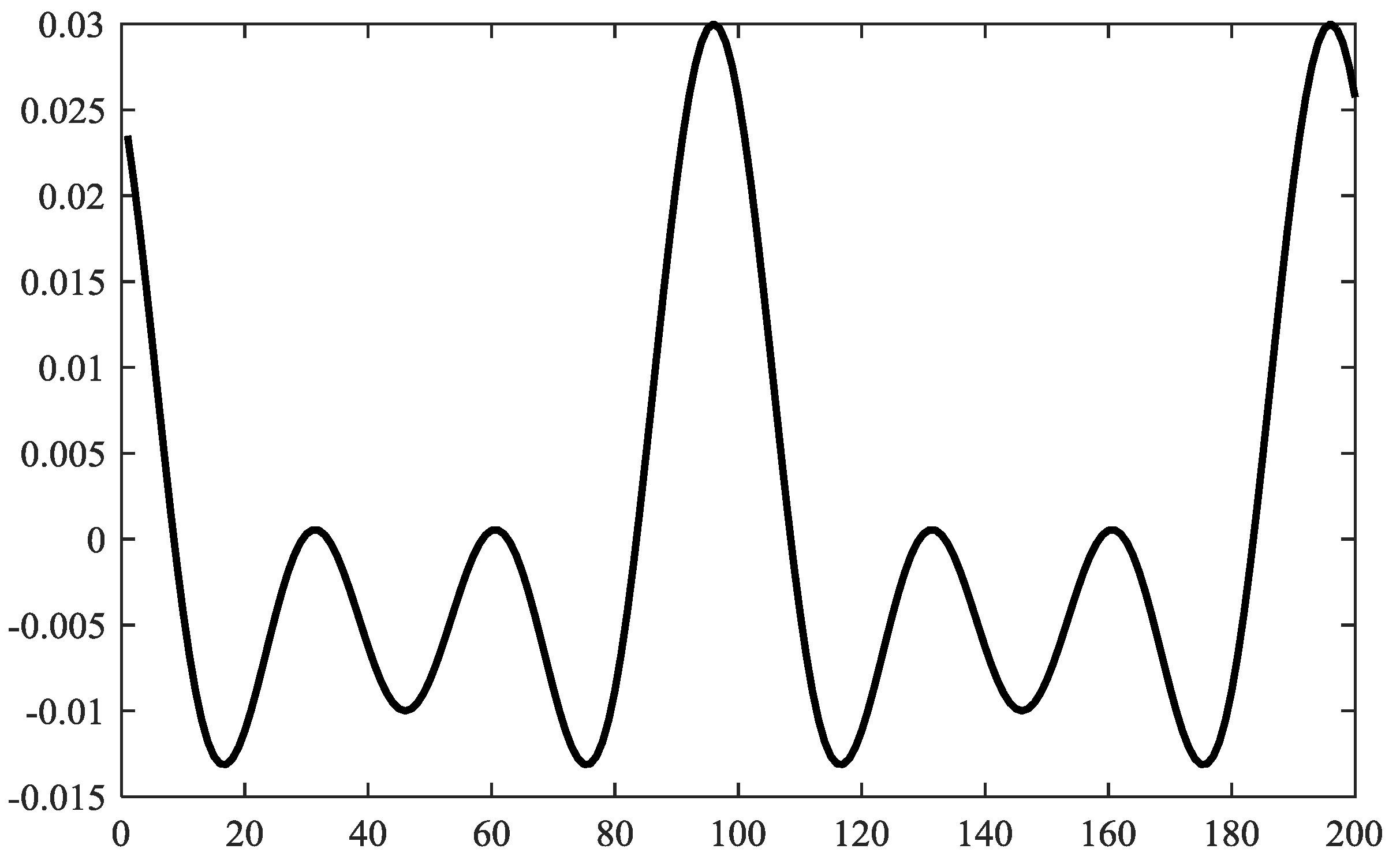
delays are required to have zero phase shift at the desired frequencies. The output vector
is obtained by multiplying the DCT coefficients calculated offline with the shift register. The DCT coefficients obtained are shown in
Figure 17. The overall control scheme using a repetitive controller is shown in
Figure 18.
4.3. Stationary Reference Saturator
As shown above, the output voltage reference of the circulating current controller is added to the output voltage reference of the current controller. Since each controller uses different phase angles both outputs can only be added in the -axis or in the -axis. In this paper it is proposed to sum both signals in -axis in order to implement saturators more easily.
In the literature it is difficult to find studies where the voltage reference saturation focused in MMCs are shown. One approach to limit the voltage reference is to limit the output of each controller independently, sum them together and apply the obtained reference to the PWM generator. However, this approach has the disadvantage of that the is not possible to guarantee that the sum of both controllers is inside the limit circle, whose radius is . Another approach is to limit the sum of both controllers. Nevertheless, this approach distorts the output reference since the waveform peaks are clipped. This distortion generates undesired harmonics and reduce the performance of the controllers.
In the paper, the use of the distortion-free saturators based on stationary reference frames (SRFs) is proposed. In particular, the saturators proposed in [
20]. The SRF saturators reduce the amplitude of the signal while maintaining the original waveform. Thus, the amplitude of the harmonics existing in the reference waveform remains the same. Thereby both current controller and circulating current controller have the same priority.
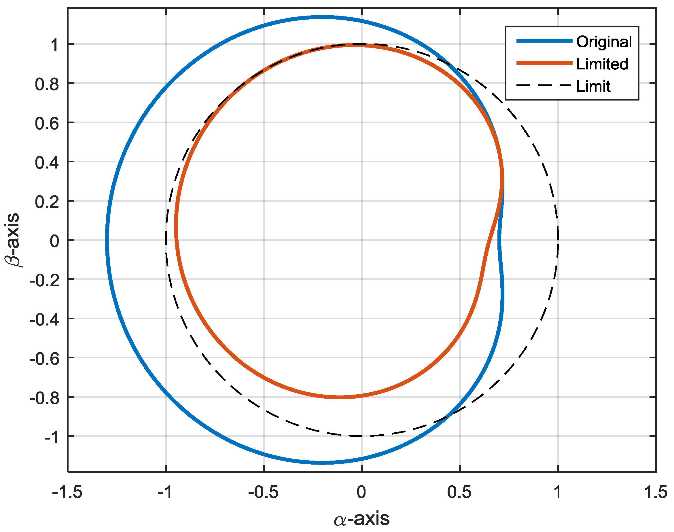
The operating principle of the SRF saturator is based on getting the complete trajectory of the vector along a complete period and fully readapting it to the limit circle if necessary. The reduction factor is constant along the whole trajectory thus, the sinusoidal waveforms are preserved.
Figure 19 shows the SRF saturator operation. The figure shows the original signal and the limited signal with the proposed saturator. As demonstrated in the figure, the entire trajectory is reduced rather than only the parts which are outside the limit. Consequently, the distortion caused by the saturator is lower.
5. Experimental Setup
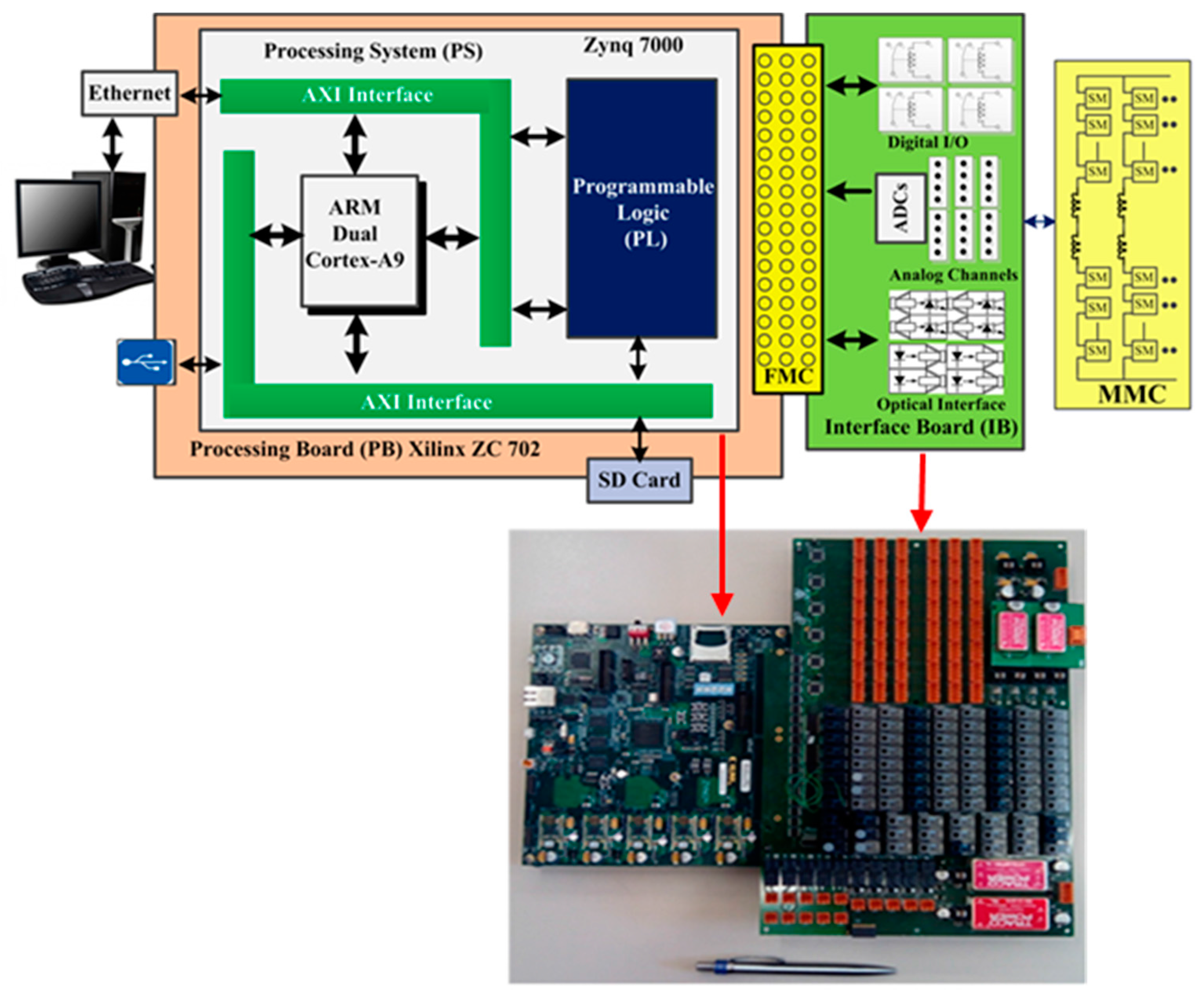
The proposed controllers discussed above have been implemented in a real processing platform designed by the authors to control multilevel converters. The used processing platform consists of two interconnected boards: the processing board and the interface board. The processing board, which is the core of the control system, is the ZC702 evaluation board manufactured by Xilinx (San José, CA, USA) that is based on a Z-7020 System-On-Chip (SoC). The Z-7020 consists of a dual-core ARM Cortex A9 (ARM, Cambridge, UK) and a FPGA. The interface board is a custom board designed by the authors which adapts the signals sent and received by the converter. The processing platform is shown in
Figure 20. Both controllers have been implemented in C code.
The first test consists of measure the computational burden of each controller. The computation burden of each controller is a key factor which is not usually addressed in the literature and has been studied in this paper. This is especially important if they are used along with more controllers in order to meet the control time constraints. In order to obtain the execution time required by each controller, a timer is used to count the clock ticks. The computational burden of both controllers is shown in
Table 1.
The results have been shown that the repetitive controller requires more time to complete the task, in fact about 10 times more than the resonant controllers. This is due to the large amount of multiplication operations required by the DCT block. However, the harmonics that can be compensated in the case of the repetitive controllers are greater than in the case of resonant controllers.
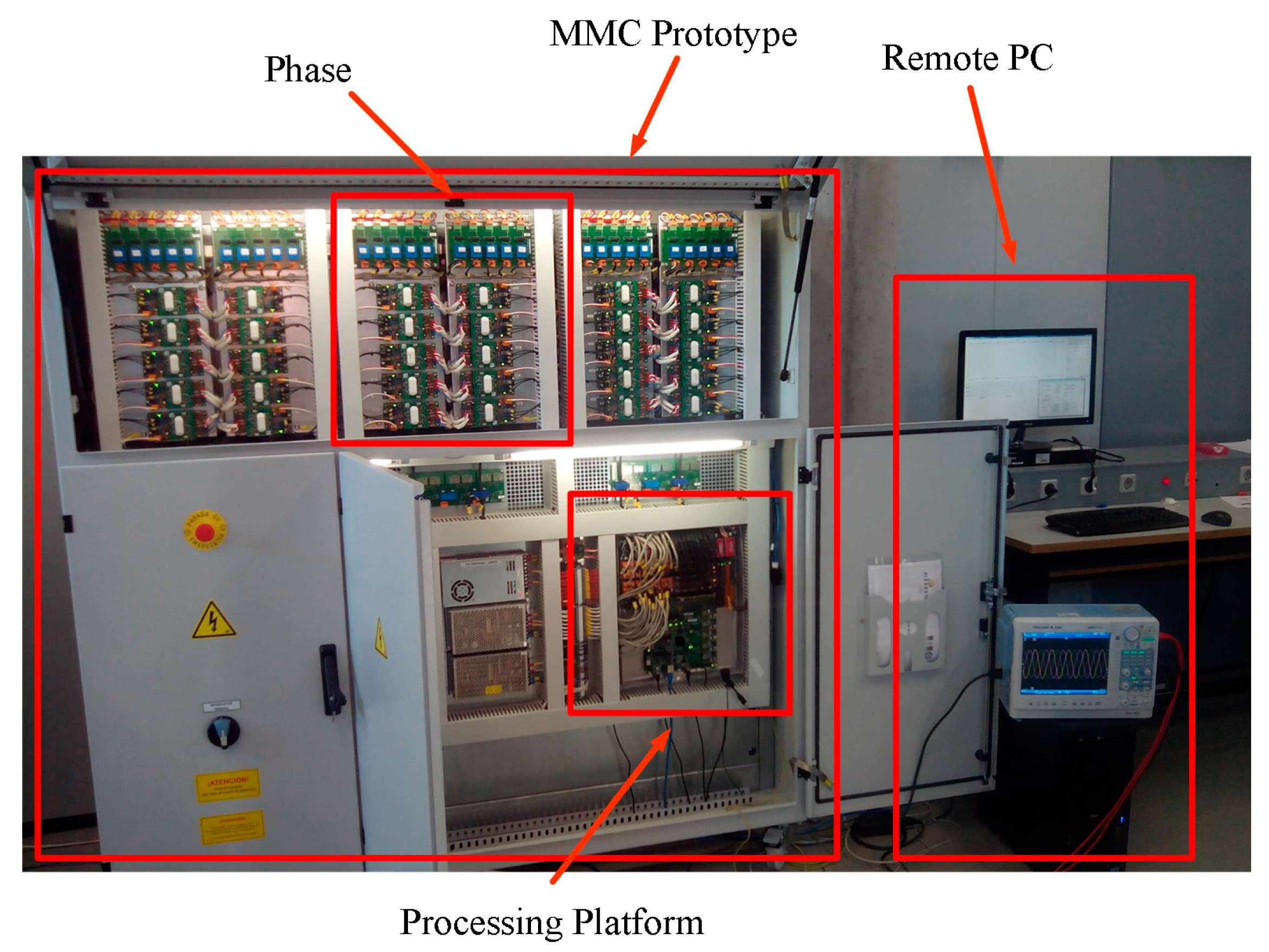
The second test consists of measuring the performance of each proposed controller. In order to achieve this, both resonant controllers and repetitive controller have been tested in a MMC prototype. The built prototype is a six-level MMC converter. Each phase consists of 10 half-bridge IGBT modules. Therefore, the entire converter has 30 half-bridge IGBT modules. A complete description is shown in
Table 2. The nominal power of the designed prototype is 50 kW.
Figure 21 shows an image of the whole prototype together with the PC that acquires the signals and controls the converter.
The prototype allows raising the DC-bus voltage up to 1200 V, therefore is possible to use this converter in 690 V grids without transformers. Moreover, the IGBTs chosen have a rated current of 150 A and a maximum voltage of 600 V. As result, this prototype can be used in a wide range of applications. The control loop has a sample rate of 100 µs. The modulation technique used is the phase-shifted sinusoidal pulse width modulation. However, other modulation techniques can be used [
21].
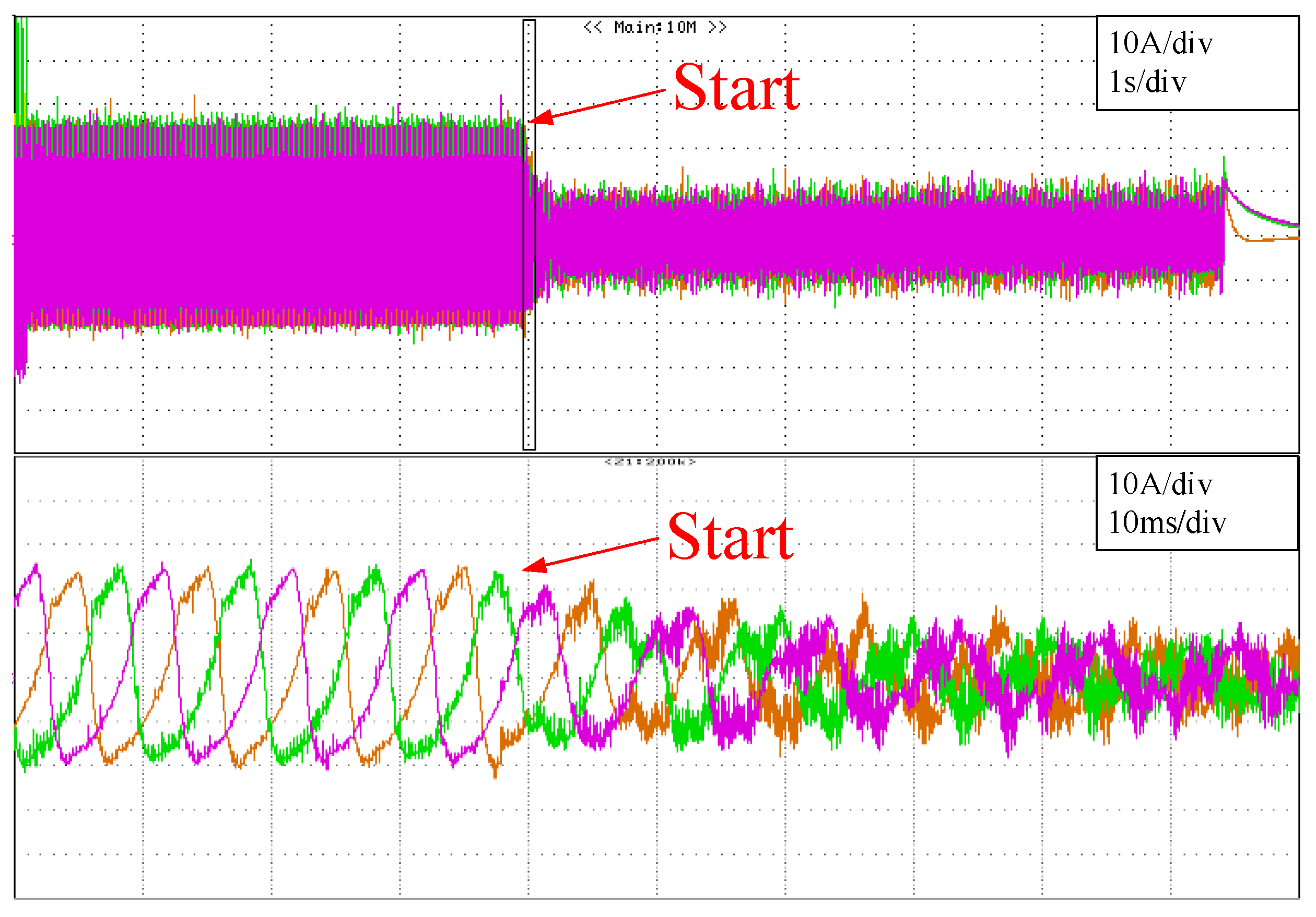
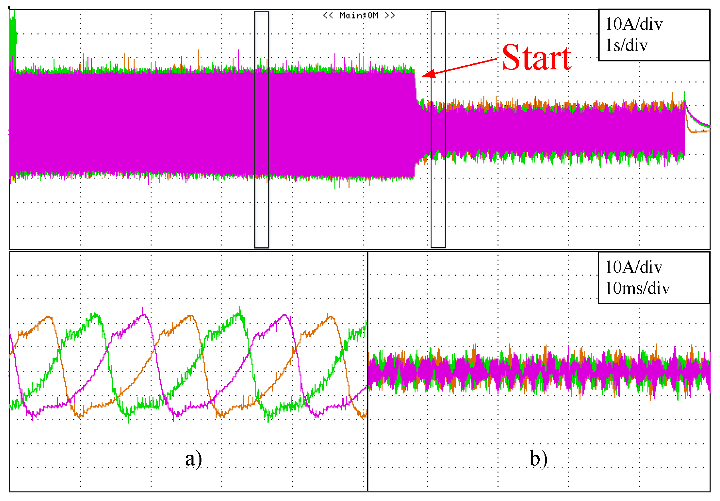
Firstly, a test to evaluate the resonant controllers has been carried out. The test consists of injecting active power to a 15 kW load and during the test, activating the resonant controllers in order evaluate the controller performance. The circulating current and the arm current are measured. The circulating current reduction are shown in
Figure 22 and
Figure 23.
Figure 22 shows how the circulating current changes when the resonant controllers are active. The figure shows that the amplitude of the circulating current is greatly reduced. This can also be observed in
Figure 23, where the circulating current without the resonant controllers and with the resonant controllers activated are shown.
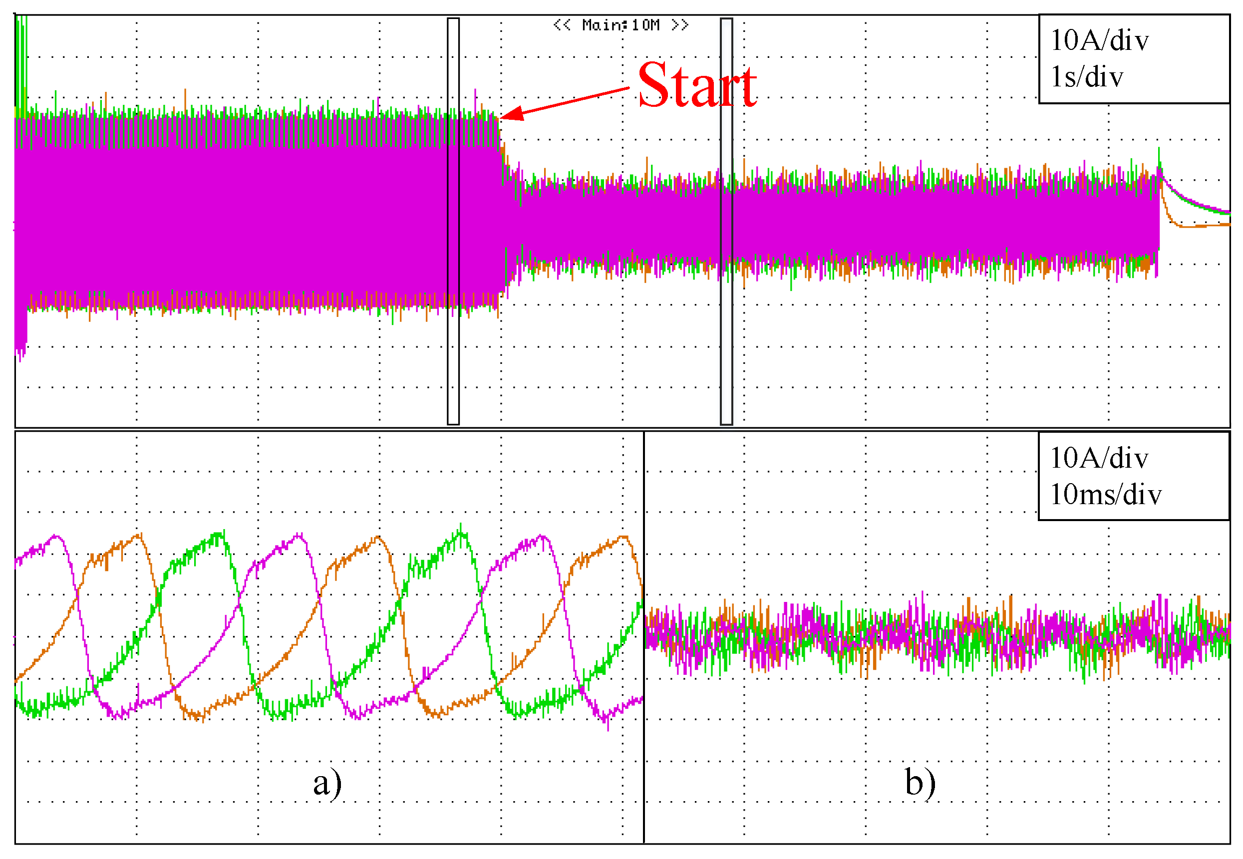
Figure 24 shows the arm current during the test. Firstly, the arm current is composed of the fundamental harmonic and the harmonics present in the circulating current. Once the resonant controllers have been activated, the harmonics generated by the circulating current are reduced and thus, the arm current is only composed of the fundamental harmonic.
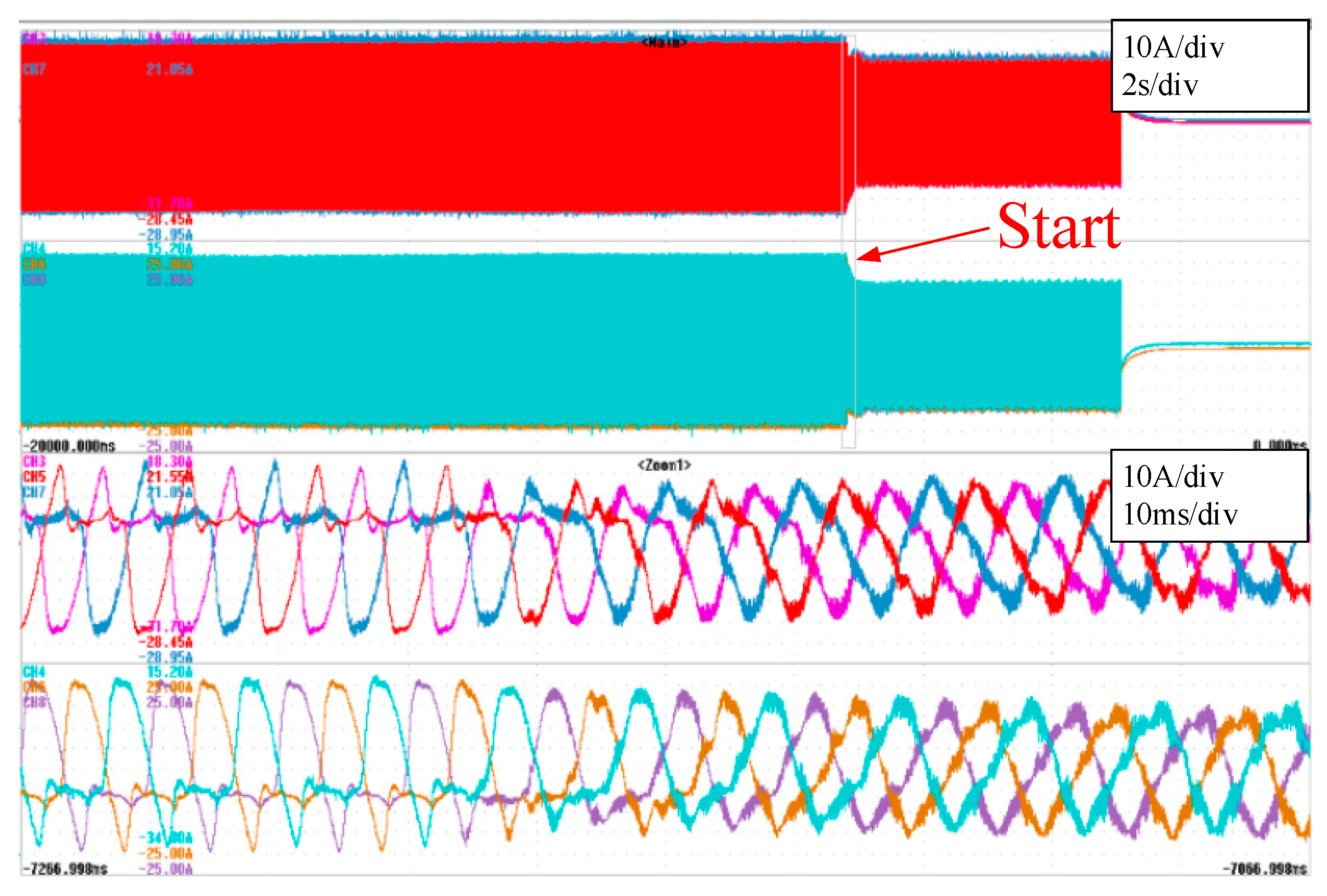
Finally, the second test consist of evaluate the repetitive controller in the same conditions as in the case of the resonant controller test.
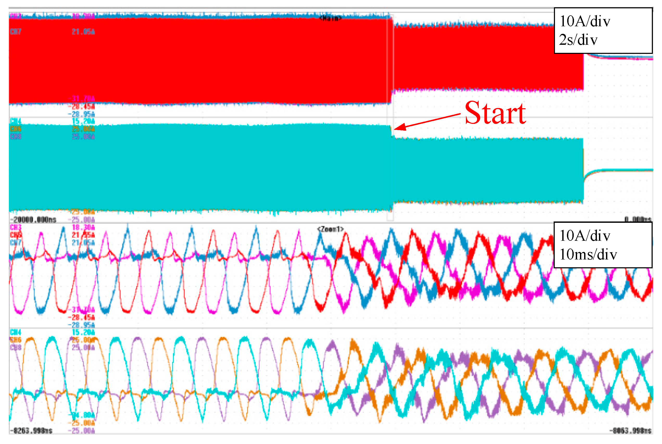
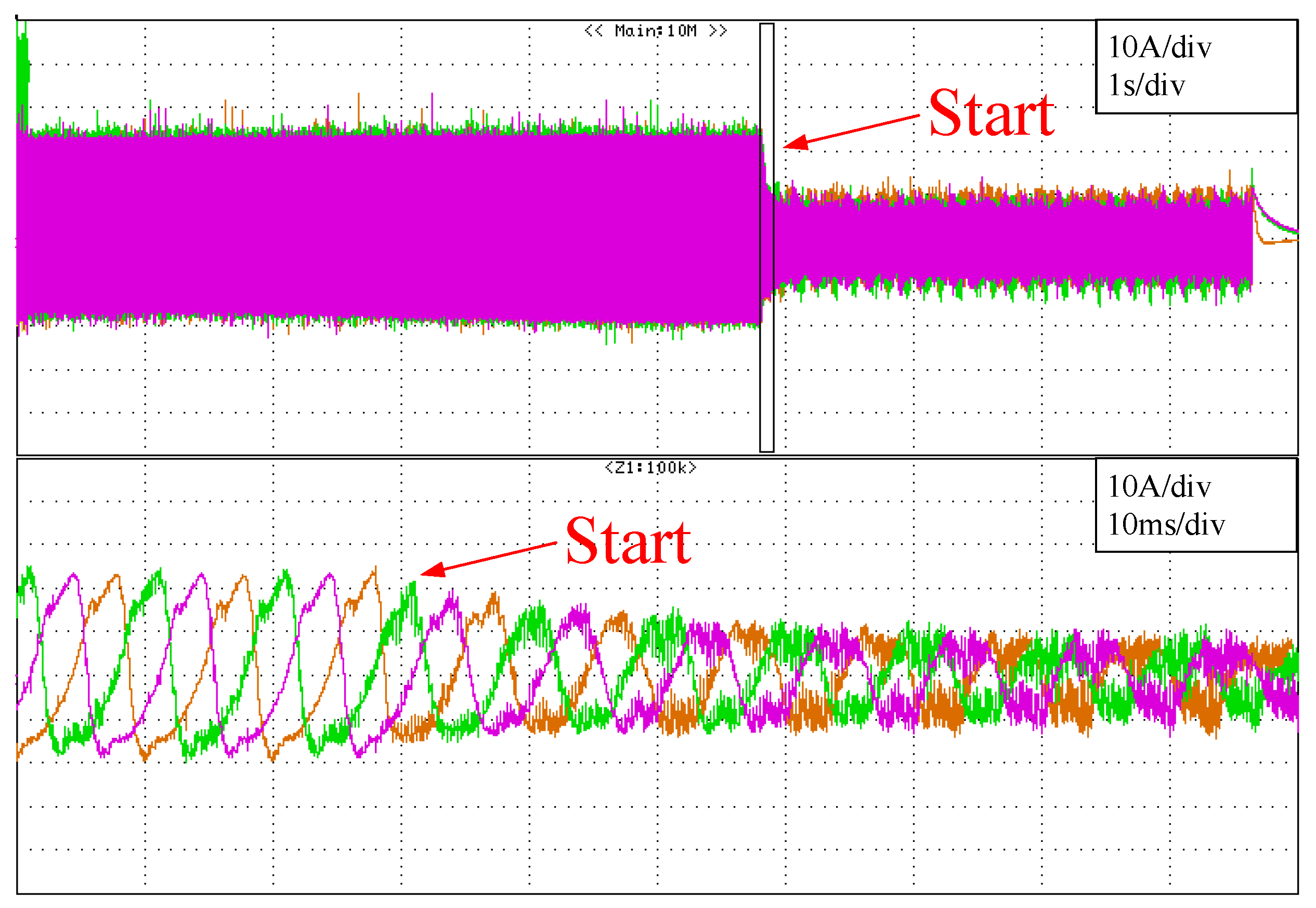
Figure 25 and
Figure 26 show the circulating current reduction when the repetitive controller is activated. In both scenarios, the resonant controllers test and the repetitive controller test, the circulating current is reduced significantly.
Figure 27 shows the arm current waveform when the repetitive controller is activated. The figure shows that in the same manner as in the case of the resonant controllers, when the repetitive controller is activated, the harmonics present in the arm current disappear and then the current only has the fundamental harmonic.
Table 3 shows the total harmonic distortion (THD) of the grid current in three scenarios: without any controller, with the resonant controllers, and with the repetitive controller. The table shows that there is a substantial reduction in the THD when any of both controllers are used. Moreover, the results shown in the table demonstrate that the THD quality improvement is similarly with both controllers.
The experimental results mentioned above show that both approaches minimize the circulating current while improving the grid quality. The resonant controllers and the repetitive controller produce similar results, but the computational cost of the repetitive controller is considerably higher than in the case of the resonant controllers.
6. Conclusions
The circulating current is an undesirable current that reduces MMC performance and increases the power losses. Thus, this current must be reduced in order to improve the efficiency. The circulating current distorts the arm current and increases its amplitude. Consequently, the power losses in the inductors increases. Moreover, due to the increased amplitude, the inductors can be saturated prematurely.
In this paper two new approaches to control the circulating current controllers in the αβ-frame have been shown. As demonstrated in this paper, the use of controllers based on the αβ-frame is the best option when there are several harmonics in the current that must be compensated. The resonant controllers and the repetitive controller have been chosen as circulating current controllers. Both controllers have been described and then tuned in order to reduce the circulating current. Moreover, a saturator which reduces the distortion when the output voltage reference must be limited has been presented. The use a saturator is an important issue that has not been well enough studied in the despite it directly affects to the performance of the controllers.
The experimental results carried out in the prototype have demonstrated the effectiveness of the proposed controllers, both the resonant controllers and the repetitive controller. The results show that the circulating current is greatly reduced when either of the proposed controllers are used. In addition, the results have been shown that the use of circulating current controllers increases the grid current quality. Consequently, the use of circulating current controller is recommended, particularly when the MMC is intended to be used in FACTS applications, where the power quality is the most important thing.


