Day-Ahead Scheduling Considering Demand Response as a Frequency Control Resource

Abstract

The development of advanced metering technologies makes demand response (DR) able to provide fast response services, e.g., primary frequency control. It is recognized that DR can contribute to the primary frequency control like thermal generators. This paper proposes a day-ahead scheduling method that considers DR as a frequency control resource, so that the DR resources can be dispatched properly with other resources. In the proposed method, the objective of frequency control is realized by defining a frequency limit equation under a supposed contingency. The frequency response model is used to model the dynamics of system frequency. The nonlinear frequency limit equation is transformed to a linear arithmetic equation by piecewise linearization, so that the problem can be solved by mixed integer linear programming (MILP). Finally, the proposed method is verified on numerical examples.

1. Introduction

Demand response (DR) is the change of the electric demand in response to the grid. Conventionally, DR is considered as a peak-load decreasing strategy, and is used for off-line planning and day-ahead scheduling. By offering customers time-varying prices, or financial incentives, the customers reduce peak load demand, so that the grid reliability is enhanced. Not only customers, but also load-serving entities and system operators can benefit from DR. By solving the day-ahead scheduling problem with DR, system operators dispatch the DR and other resources properly, minimizing the total operation cost and at the same time meeting the system equations. The day-ahead scheduling problem with DR has been investigated in many research works. For example, the scheduling problems with price-elastic DR are investigated in [1,2,3], and some other studies incorporate DR with renewable energies in scheduling problems [4,5].

In recent years, based on advanced metering technologies, DR is able to provide real-time ancillary services, such as primary frequency control. Since the system frequency reflects the real-time balance between the electric power supply and the demand, DR can support this balance through managing the demand side resources. For example, when the frequency decreases, some electrical appliances are switched off or reduce their load demand temporarily to help the frequency restore to the nominal value. It is demonstrated that DR can perform like thermal generators in the frequency control. Unlike conventional under-frequency load shedding (UFLS), the electrical appliances that participate in the frequency control are usually non-essential loads. These loads can provide immediate response without causing any inconvenience to residents. During recent years, increasing attention have been paid to DR in the frequency control. A variety of control strategies, e.g., decentralized control strategies [6,7], centralized control strategies [8,9], hybrid hierarchical control strategies [10], proportional-integral (PI) control method [11,12], linear quadratic regulator method [13], H_∞ control method [14], etc., have been developed. Some researches incorporate DR with other resources in the frequency control, e.g., wind generators [15], storages [16], etc. Some other researches apply DR to real power systems, to test its performance in the frequency control [17,18].

However, very few studies take DR as a frequency control resource in the scheduling problem. Although [19] proposes a method that incorporates DR as part of the spinning reserve in the scheduling problem, system reserves are usually activated within minutes or more. The primary frequency control, which should act in a very short time to cope with transient disturbances, is not discussed in [19].

Moreover, DR for the load shifting (load-shifting DR for short) and DR for the frequency control (frequency-control DR for short) are investigated separately, and few studies incorporate the two kinds of DR services together. On the one hand, the system frequency response characteristics are usually dependent on the scheduling results; on the other hand, some DR resources that participate in frequency control can also provide load decreasing or shifting services, and it is necessary to develop a method to dispatch the different kinds of DR resources properly.

In view of the above, this paper proposes a scheduling method considering DR as a frequency control resource. DR can provide not only the load-shifting, but also primary frequency control. With the proposed method, the DR resources for both load-shifting and frequency-control can be properly dispatched. The remainder of this paper is organized as follows: In Section 2, the day-ahead scheduling problem with both frequency-control DR and load-shifting DR is formulated. In Section 3, the frequency limit equation considering DR is modeled. Case studies are provided in Section 4. Finally, conclusions are summarized in Section 5.

2. Day-Ahead Scheduling with Flexible Demand Response (DR) Resources

DR is a flexible resource that can support the stability of the power system in different time scales. For a long time scale, DR can provide peak clipping or load-shifting at peak hours. For a short time scale, DR can support the primary frequency control. In the scheduling problem, we consider these two different kinds of services from DR.

The DR programs have been classified into two major categories, namely, incentive-based DR and price-based DR. Incentive-based DR refers to customers receiving payments or preferential prices for offering DR, whereas price-based DR allows customers to voluntarily adjust their demand based on varying electricity price. In our model, both price-based DR and the incentive-based DR are considered. The load-shifting DR is based on the time-varying price, whereas the frequency-control DR is based on the financial incentive.

The price-based DR for load-shifting has been investigated in many research works [1,2,3,20]. The time-varying electricity price makes the consumers shift their demand from the peak hours to other durations. Due to the page limit, this paper does not discuss the price-based load-shifting DR in detail. In this paper, the modeling of the load-shifting DR takes the similar approach as [3].

The incentive-based DR for the frequency-control is managed by the aggregator through a technical unit named as virtual power plant (VPP). The contracts between the aggregators and the electric consumers will allow the aggregators to manage the electricity consumption of the DR appliances. In addition, the consumer will get some payments in return. Since these payments will add costs to the system operators, the cost should be considered in the scheduling. In this paper, the DR cost for frequency control is based on the capacity of the dispatched frequency-control DR.

The goal of the scheduling problem is to determine the schedule of generators and the DR resources, so that the total social welfare is maximized [1,2,3,20]. Considering DR in the load-shifting and frequency control, the objective function can be formulated as below:

$$\text{max} {\displaystyle \sum _{h=1}^{N_{\mathrm{h}}}{\displaystyle \sum _{nl=1}^{N_{\mathrm{nl}}}{p}_{h,nl}^{\text{LDR}}\cdot ld{r}_{h,nl}}}-\left({\displaystyle \sum _{h=1}^{N_{\mathrm{h}}}{\displaystyle \sum _{i=1}^{N_{\mathrm{g}}}\left(C(P_{i,h})+S{U}_{i,h}+S{D}_{i,h}\right)}}+{\displaystyle \sum _{h=1}^{N_{\mathrm{h}}}{\displaystyle \sum _{nf=1}^{N_{\text{nf}}}{p}_{h,nf}^{\text{FDR}}\cdot fd{r}_{h,nf}}}\right)$$

(1)

The first term and the second term in Equation (1) are, respectively, the consumer gross surplus and the system operation cost [1,2,3,20]. The consumer gross surplus is only related to price-based DR (which is for load shifting). The system operation cost mainly includes two parts: the generation cost and the DR cost. The generation cost consists of fuel cost, start-up cost and shut-down cost, and the DR cost is what the system operator pays the aggregators for offering frequency-control DR.

The optimization problem is subject to the following equations:

(1) Generation Operation Equations

$${\displaystyle \sum _{i=1}^{N_{\mathrm{g}}}{P}_{i,h}}=D_h-LD{R}_h$$

(2)

$$u_{i,h}\cdot P_i^{\text{min}}\le P_{i,h}\le u_{i,h}\cdot P_i^{\text{max}}$$

(3)

$$-R{D}_i\le P_{i,h}-P_{i,h-1}\le R{U}_i$$

(4)

$$x_{i,h}-y_{i,h}=u_{i,h}-u_{i,h-1}$$

(5)

$$x_{i,h}+y_{i,h}\le 1$$

(6)

The generation operation equations are listed in (2)–(6). Equations (2)–(4) are, respectively, the power balance equation, generating unit limit equation, and ramp rate limit equation. Equations (5) and (6) are the state transition equations, which define the relationship between the binary start-up variable x_i,h, binary shutdown variable y_i,h, and binary commitment variable u_i,h.

(2) DR Equations

$$0\le LD{R}_h\le LD{R}_h^{\text{max}}$$

(7)

$$0\le FD{R}_h\le FD{R}_h^{\text{max}}$$

(8)

$$0\le LD{R}_h+FD{R}_h\le D{R}_h^{\text{max}}$$

(9)

$$0\le {\displaystyle \sum _{h=1}^{N_{\mathrm{h}}}LD{R}_h}\le E^{\text{max}}$$

(10)

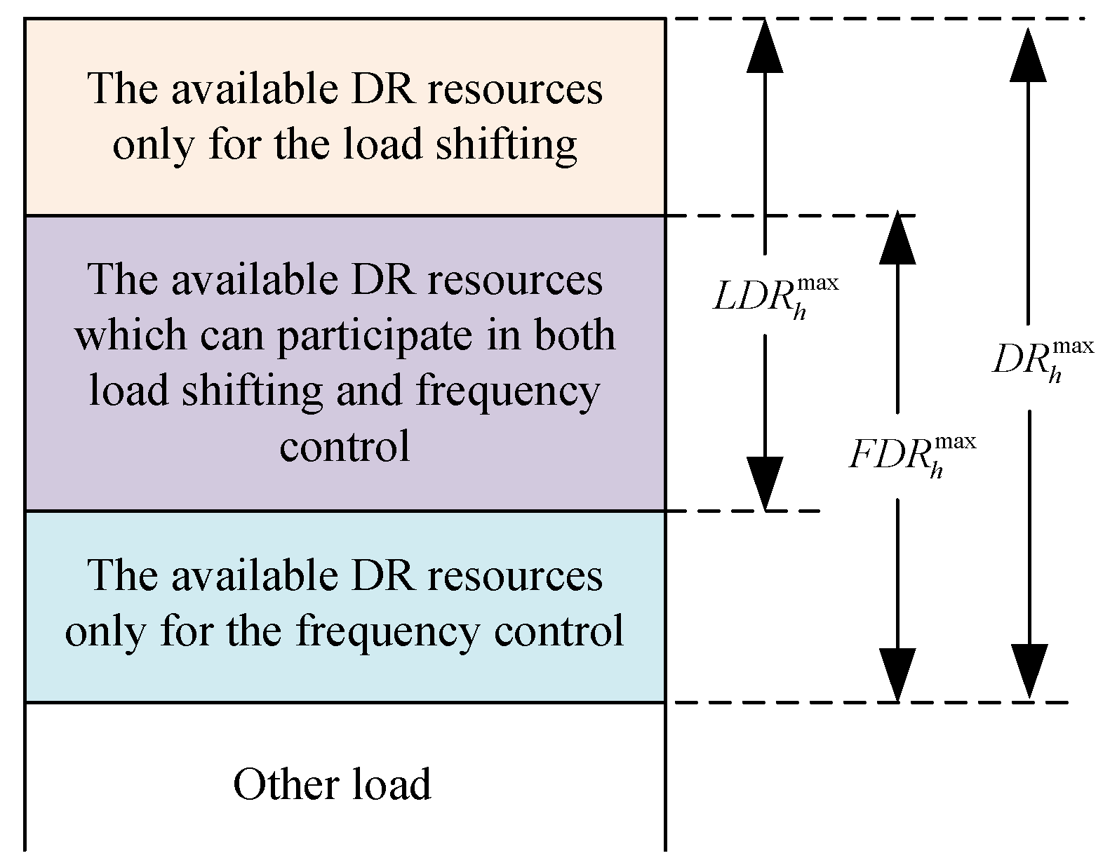
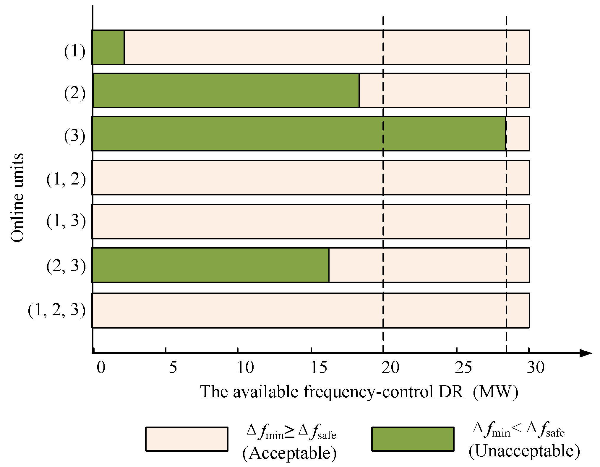
The DR equations are listed in Equations (7)–(10), Equations (7) and (8) define the maximum limits of the dispatched DR for load-shifting and DR for frequency control, respectively. Equation (9) defines the limits of the total amount of dispatched DR for load-shifting and frequency control. Note that frequency-control DR and load-shifting DR are not independent from each other. Some of the DR resources that participate in the load-shifting can at the same time support frequency control. The relationship between the maximum available DR resources and the load-shifting and frequency control is shown in Figure 1.

Equation (10) imposes a limit to the total allowable load change over the scheduling period 3. The curtailed load will be fully shifted to other periods if E^max is set at 0.

(3) System Frequency Equation

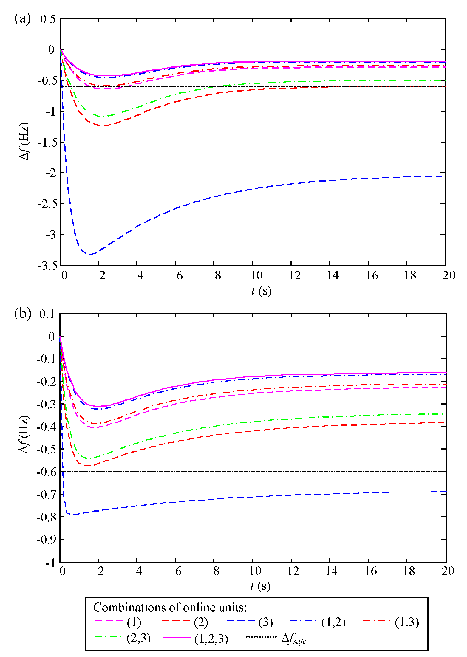
System frequency reflects the balance between the electric power supply and consumption. When there is imbalance between electric supply and demand, system frequency will increase or decrease. Generally, system frequency control can be separated into primary, secondary, and tertiary control. Primary control is proportional feedback control that operated by the speed governors of the generation units. It takes the first step to intercept the load frequency fluctuation. Secondary control is performed by some selected generators that adjust the load frequency to the nominal value. Tertiary control is activated manually to release the secondary control reserves. Among primary, secondary, and tertiary control, the primary control is to compensate large and sudden disturbances. In this paper, we focus on the primary frequency control by DR.

In our model, the task of the primary frequency control is constraining the frequency in the expected normal range when a sudden disturbance occurs. If the frequency drops too low (e.g., 0.6Hz lower than the nominal frequency), UFLS may operate to avoid system collapse. However, UFLS will cause power failure to the power consumers. To avoid trigging UFLS, it is necessary to consider the primary frequency control in the scheduling problem. Usually, the primary frequency control is incorporated in the scheduling problem by defining a reserve equation [21,22]. Though easily modeled, the primary reserve only reflects the steady-state frequency deviation in about 5 to 10 s. However, the maximum system frequency drop cannot be reflected. In many cases, the under frequency relay triggers instantly when the system frequency is detected below one threshold. Therefore, in order to avoid trigging UFLS, it is necessary to consider the frequency limit equation instead of the reserve equation.

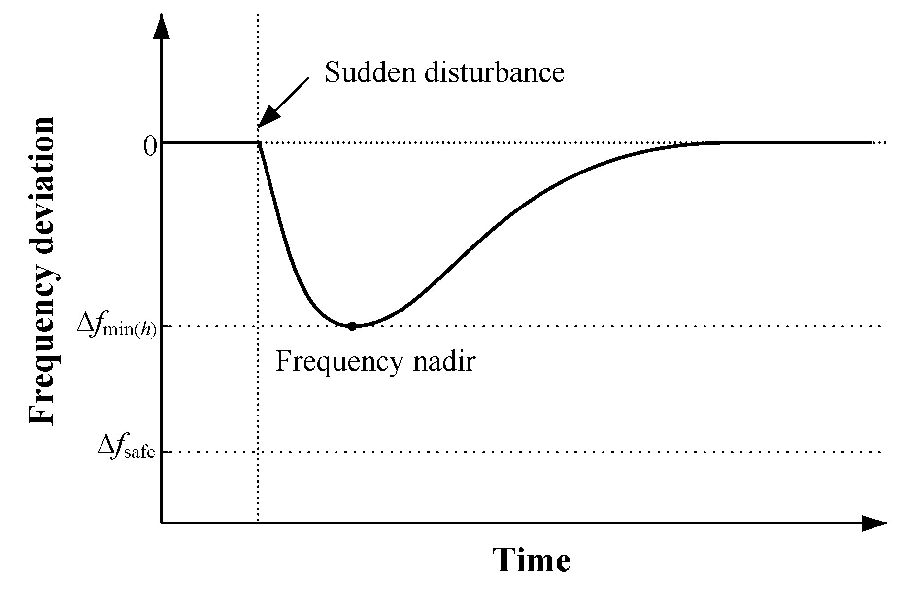
To model the frequency limit equation, here we define a safe frequency level Δf_safe, shown in Figure 2. For a supposed contingency (e.g., 10% generation loss or the frailer of the largest generator), the frequency nadir should be above Δf_safe [8]. The system frequency limit equation is defined in Equation (11).

$$\Delta f_{\text{min}(h)}\ge \Delta f_{\text{safe}}$$

(11)

However, Equation (11) is not easy to calculate due to the non-linear nature of the system frequency response characteristic. The details about calculating the frequency limit equation are presented in the next section.

3. Frequency Limit Equation Modeling

The purpose of this section is to find a way of modeling the frequency limit equation, and transform the frequency limit equation into an inequality relationship between u_i,h and FDR_h.

3.1. Calculation of the Frequency Nadir

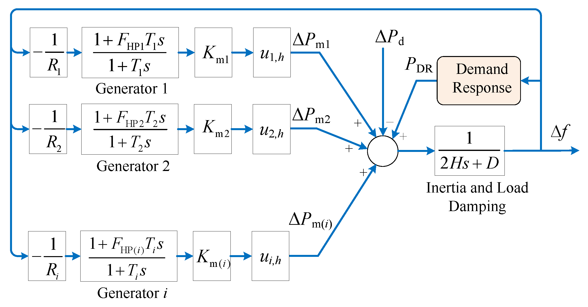
The frequency response model is an effective tool to study the dynamic characteristics of the frequency in response to the time-varying supply or demand. Figure 3 shows a low order frequency response model with multiple generator units. Note that u_i,h is the unit commitment (UC) parameter, which was introduced in Section 2. Since this paper focuses on the primary frequency control of the scheduling problem, in Figure 3 each generation unit is equipped with a governor system. Because the response time of secondary frequency control could be a minute or two (much longer than the response time of primary control), the secondary frequency control is not involved in Figure 3.

According to Figure 3, the function of ∆f can be derived as following:

$$\Delta f(s)=\frac{-\Delta P_{\mathrm{d}}(s)+P_{\text{DR}}(s)}{(2Hs+D)+{\displaystyle \sum _{i=1}^{N_{\mathrm{g}}}\frac{K_{\mathrm{m}(i)}\cdot u_{i,t}\cdot (1+F_{\text{HP}(i)}{T}_{i}s)}{R_i(1+T_{i}s)}}}$$

(12)

Sudden disturbances usually take the form of a step function:

$$\Delta P_{\mathrm{d}}(s)=\frac{P_{\text{step}}}{s}$$

(13)

where P_step denotes the disturbance magnitude.

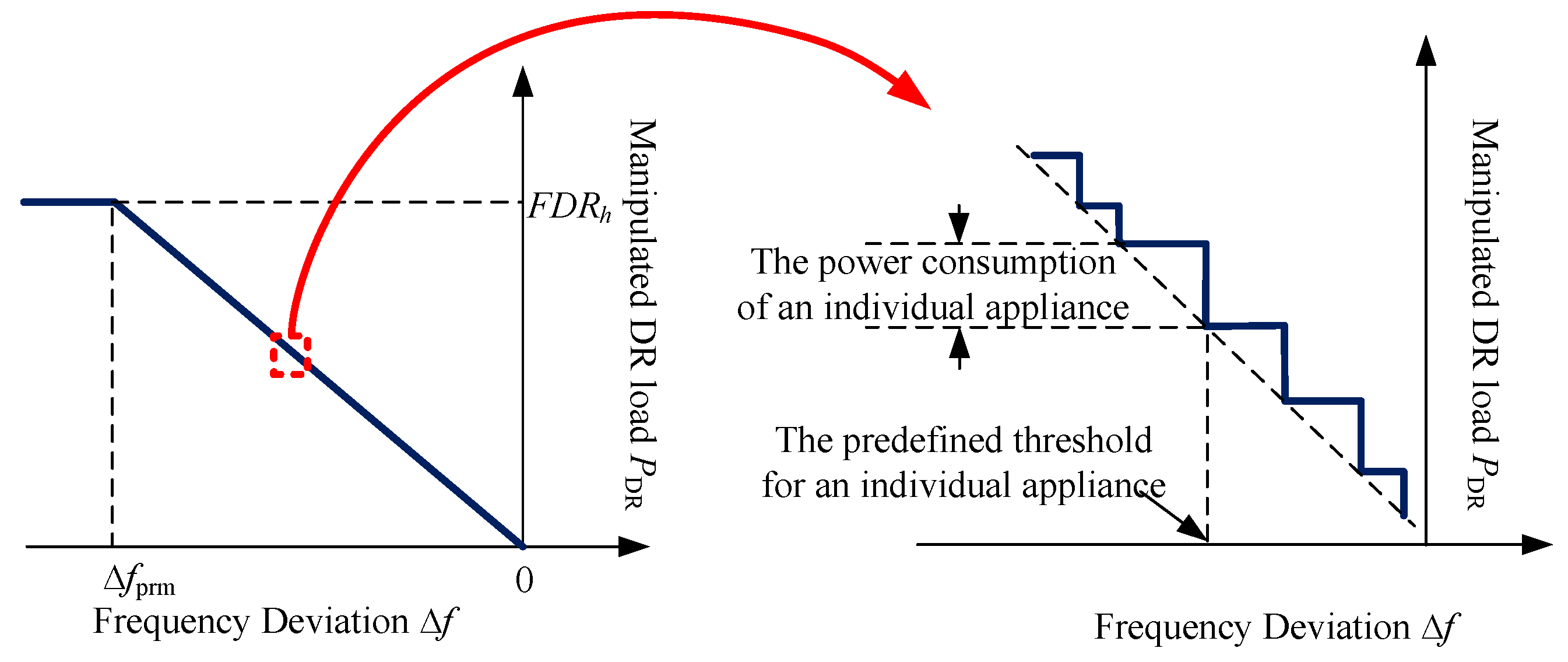
The effect of DR in the frequency control has been studied in many earlier researches. To provide primary frequency control, the manipulated responsive DR for the frequency control should be based on the frequency deviation [10,23]. For a negative frequency deviation ∆f < 0, the amount manipulated DR is determined by:

$$P_{\text{DR}}=\{\begin{array}{ll}-k_{\text{DR}}\Delta f& \text{If} \Delta f_{\text{prm}}\le \Delta f\le 0\\ P_{\text{DRm}}& \text{If} \Delta f<\Delta f_{\text{prm}}\end{array}$$

(14)

where k_DR is a pre-defined parameter, which is calculated as:

$$k_{\text{DR}}=-\frac{FD{R}_h}{\Delta f_{\text{prm}}}$$

(15)

where ∆f_prm is the frequency deviation at which all the primary reserves are delivered and FDR_h is the available frequency-control DR, which was introduced in Section 2.

Note that the DR may not give a continuous response like Equation (14) because most of the appliances that participate in DR are ON/OFF appliances (i.e., refrigerators, freezers, and water heaters without frequency variation speed control) that can only provide a discrete response. To implement DR with these appliances, a number of frequency thresholds are usually set in advance. If one controller detects ∆f below a predefined threshold ∆f_th, the controller outputs a switching signal and switches the appliance off. However, we can define different ∆f_th for different appliances properly so that their aggregated frequency response characteristic is similar to Equation (14), as can be seen in Figure 4. The overall control framework can be based on a hierarchical framework [10] that combines the centralized and decentralized control framework together. In such a control framework, individual controllers measure the system frequency and compute control signals by themselves; meanwhile, the control parameters are given by the control centre. The response delay is very small and can be neglected [10]. More details of this DR control strategy can refer [10].

To ensure a large enough frequency regulation range, the parameter ∆f_prm should be below or at least equal to the safe frequency level ∆f_safe. If we do not consider the situation that ∆f < ∆f_prm, P_DR(s) can be expressed as following:

$$P_{\text{DR}}(s)=-k_{\text{DR}}\Delta f(s)$$

(16)

Equation (16) neglects the dynamics of DR. If there exists a communication delay of DR, a pure delay $e^{-s\cdot T_{\mathrm{d}}}$ is needed to be considered in Equation (16): $P_{\text{DR}}(s)=-k_{\text{DR}}\cdot e^{-s\cdot T_{\mathrm{d}}}\cdot \Delta f(s)$. However, in a hierarchical control framework such as [10], the response delay of DR is so small that can be neglected.

Substituting Equations (13) and (16) in Equation (12) yields

$$\Delta f(s)=-\frac{P_{\text{step}}}{s\left((2Hs+D+k_{\text{DR}})+{\displaystyle \sum _{i=1}^{N_{\mathrm{g}}}\frac{K_{\mathrm{m}(i)}\cdot u_{i,t}\cdot (1+F_{\text{HP}(i)}{T}_{i}s)}{R_i(1+T_{i}s)}}\right)}$$

(17)

It can be seen from (17) that the introduction of DR is equivalent to adding the load-damping factor D of the frequency response model. By assuming an identical T_E instead of T_i for all the generators [24], Equation (17) can be simplified as follows

$$\Delta f(s)=-\frac{P_{\text{step}}}{s\left((2Hs+D+k_{\text{DR}})+\frac{K_{\mathrm{R}}+K_{\mathrm{F}}{T}_{\mathrm{E}}s}{1+T_{\mathrm{E}}s}\right)}$$

(18)

where

$$K_{\mathrm{R}}={\displaystyle \sum _{i=1}^{N_{\mathrm{g}}}\frac{K_{\mathrm{m}(i)}\cdot u_{i,h}}{R_i}}$$

(19)

$$K_{\mathrm{F}}={\displaystyle \sum _{i=1}^{N_{\mathrm{g}}}\frac{K_{\mathrm{m}(i)}\cdot F_{\text{HP}(i)}\cdot u_{i,h}}{R_i}}$$

(20)

Note that the parameters K_R, K_F are functions of u_i,h. And the parameter H is also a function of u_i,h. H can be calculated by:

$$H={\displaystyle \sum _{i=1}^{N_{\mathrm{g}}}{K}_{\mathrm{m}(i)}\cdot H_i\cdot u_{i,h}}$$

(21)

By computing the inverse Laplace transform of Equation (18), the time domain equation can be obtained as follows

$$\Delta f(t)=-\frac{P_{\text{step}}}{(D+k_{\text{DR}})+K_{\mathrm{R}}}\times (1-\frac{1}{\sqrt{1-{\varsigma }^2}}{e}^{-\varsigma {\omega }_{\mathrm{n}}t}\text{sin}({\omega }_{\mathrm{r}}t+\phi )+\frac{T_{\mathrm{E}}{\omega }_{\mathrm{n}}}{\sqrt{1-{\varsigma }^2}}{e}^{-\varsigma {\omega }_{\mathrm{n}}t} \text{sin} {\omega }_{\mathrm{r}}t)$$

(22)

where

$$\varsigma =\frac{2H+(D+k_{\text{DR}})T_{\mathrm{E}}+K_{\mathrm{F}}{T}_{\mathrm{E}}}{2\cdot \sqrt{2H{T}_{\mathrm{E}}\left[(D+k_{\text{DR}})+K_{\mathrm{R}}\right]}}$$

(23)

$${\omega }_{\mathrm{n}}=\sqrt{\frac{(D+k_{\text{DR}})+K_{\mathrm{R}}}{2H{T}_{\mathrm{E}}}}$$

(24)

$${\omega }_{\mathrm{r}}={\omega }_{\mathrm{n}}\sqrt{1-{\varsigma }^2}$$

(25)

$$\phi ={\text{tan}}^{-1}\left(\frac{\sqrt{1-{\varsigma }^2}}{\varsigma }\right)$$

(26)

At the time of the frequency nadir Δf_min(h), the slope of the frequency deviation is zero. By solving dΔf(t)/dt = 0, the time of the frequency nadir t_z can be obtained as follows

$$t_{\mathrm{z}}=\frac{1}{{\omega }_{\mathrm{r}}}{\text{tan}}^{-1}\left(\frac{{\omega }_{\mathrm{r}}{T}_{\mathrm{E}}}{\varsigma {\omega }_{\mathrm{n}}{T}_{\mathrm{E}}-1}\right)$$

(27)

Substituting Equation (27) in (22), the frequency nadir can be obtained:

$$\Delta f_{\text{min}(h)}=\Delta f(t_{\mathrm{z}})$$

(28)

3.2. Piece Wise Linearization of the Frequency Limit Equation

From Equation (15) and Equations (19)–(28), we can see that Δf_min(h) is a function of u_i,h and FDR_h. However, the expression of Δf_min(h) is nonlinear and is too complicated to be solved by traditional methods, e.g., mixed integer linear programming. It is necessary to linearize the function of Δf_min(h).

Since T_E and D are predefined parameters for Equation (18), and is not directly affected by the parameters u_i,t and FDR_h. Only the four variables H, k_DR, K_F, K_R are considered in the linearization of the function Δf_min(h).

Suppose that H, k_DR, K_F, K_R have the following maximum and minimum limits:

$$H_{\text{min}}\le H\le H_{\text{max}}$$

(29)

$$k_{\text{DRmin}}\le k_{\text{DR}}\le k_{\text{DRmax}}$$

(30)

$$K_{\text{Fmin}}\le K_{\mathrm{F}}\le K_{\text{Fmax}}$$

(31)

$$K_{\text{Rmin}}\le K_{\mathrm{R}}\le K_{\text{Rmax}}$$

(32)

For linearization, the domains of H, k_DR, K_F, K_R are divided equally into ii_m, jj_m, kk_m, ll_m pieces, respectively. Therefore, the definition domain has totally ii_m×jj_m×kk_m×ll_m pieces.

Suppose that H, k_DR, K_F, K_R are in the range of ii, jj, kk, ll pieces, which is denoted as (ii, jj, kk, ll), that is:

$$H\in (H_{\text{min}}+(ii-1)\Delta H,H_{\text{min}}+ii\Delta H)$$

(33)

$$k_{\text{DR}}\in (k_{\text{DRmin}}+(jj-1)\Delta k_{\text{DR}},k_{\text{DRmin}}+jj\Delta k_{\text{DR}})$$

(34)

$$K_{\mathrm{F}}\in (K_{\text{Fmin}}+(kk-1)\Delta K_{\mathrm{F}},K_{\text{Fmin}}+kk\Delta K_{\mathrm{F}})$$

(35)

$$K_{\mathrm{R}}\in (K_{\text{Rmin}}+(ll-1)\Delta K_{\mathrm{R}}, K_{\text{Rmin}}+ll\Delta K_{\mathrm{R}})$$

(36)

Δf_min(h) can be estimated by a linear function:

$$\begin{array}{c}\Delta f_{\text{min}(h)}=A{A}_{(ii,jj,kk,ll)}H+B{B}_{(ii,jj,kk,ll)}{k}_{\text{DR}}+C{C}_{(ii,jj,kk,ll)}{K}_{\mathrm{F}}\\ +D{D}_{(ii,jj,kk,ll)}{K}_{\mathrm{R}}+E{E}_{(ii,jj,kk,ll)}\end{array}$$

(37)

where AA_{(ii, jj, kk, ll)}, BB_{(ii, jj, kk, ll)}, CC_{(ii, jj, kk, ll)}, DD_{(ii, jj, kk, ll)}, EE_{(ii, jj, kk, ll)} are parameters that are determined by least squares estimation. By introducing a large enough ε, the conditions from Equations (33)–(36) and Equation (37) can be transformed to the following equivalent linear relations:

$$-\epsilon +\epsilon \cdot v_{(ii,jj,kk,ll)}\le H_{\text{min}}+ii\Delta H-H$$

(38)

$$-\epsilon +\epsilon \cdot v_{(ii,jj,kk,ll)}\le H-\left(H_{\text{min}}+(ii-1)\Delta H\right)$$

(39)

$$-\epsilon +\epsilon \cdot v_{(ii,jj,kk,ll)}\le k_{\text{DRmin}}+jj\Delta k_{\text{DR}}-k_{\text{DR}}$$

(40)

$$-\epsilon +\epsilon \cdot v_{(ii,jj,kk,ll)}\le k_{\text{DR}}-\left(k_{\text{DRmin}}+(jj-1)\Delta k_{\text{DR}}\right)$$

(41)

$$-\epsilon +\epsilon \cdot v_{(ii,jj,kk,ll)}\le K_{\text{Fmin}}+kk\Delta K_{\mathrm{F}}-K_{\mathrm{F}}$$

(42)

$$-\epsilon +\epsilon \cdot v_{(ii,jj,kk,ll)}\le K_{\mathrm{F}}-\left(K_{\text{Fmin}}+(kk-1)\Delta K_{\mathrm{F}}\right)$$

(43)

$$-\epsilon +\epsilon \cdot v_{(ii,jj,kk,ll)}\le K_{\text{Rmin}}+ll\Delta K_{\mathrm{R}}-K_{\mathrm{R}}$$

(44)

$$-\epsilon +\epsilon \cdot v_{(ii,jj,kk,ll)}\le K_{\mathrm{R}}-\left(K_{\text{Rmin}}+(ll-1)\Delta K_{\mathrm{R}}\right)$$

(45)

$${\displaystyle \sum _{ii=1}^{i{i}_{\mathrm{m}}}{\displaystyle \sum _{jj=1}^{j{j}_{\mathrm{m}}}{\displaystyle \sum _{kk=1}^{k{k}_{\mathrm{m}}}{\displaystyle \sum _{ll=1}^{l{l}_{\mathrm{m}}}{v}_{(ii,jj,kk,ll)}}}}}=1$$

(46)

$$\begin{array}{c}-\epsilon +\epsilon \cdot v_{(ii,jj,kk,ll)}\le \Delta f_{\text{min}(h,ii,jj,kk,ll)}-(A_{(ii,jj,kk,ll)}H+B_{(ii,jj,kk,ll)}{k}_{\text{DR}}\\ +C_{(ii,jj,kk,ll)}{K}_{\mathrm{F}}+D_{(ii,jj,kk,ll)}{K}_{\mathrm{R}}+E{E}_{(ii,jj,kk,ll)})\le \epsilon -\epsilon \cdot v_{(ii,jj,kk,ll)}\end{array}$$

(47)

where v_{(ii, jj, kk, ll)} is a binary variable indicating the piece (ii, jj, kk, ll) if v_{(ii, jj, kk, ll)} is 1. Since the Equations (38)–(47) are for the piece (ii, jj, kk, ll), the system frequency equation can be expressed by:

$$\Delta f_{\text{min}(h,ii,jj,kk,ll)}\ge \Delta f_{\text{safe}}$$

(48)

The linear Equations (38)–(48) are equivalent to the Equation (11) and can be easily solved by the method of MILP.

4. Numerical Results

In this section, numerical case studies are performed on a six-bus system and the 17-unit system to test the proposed method. The day-ahead scheduling problems are solved by using the CPLEX software.

4.1. Six-Bus System

The six-bus system has three thermal generator units [24,25]. The frequency response characteristics of generators are listed in the Appendix A (

Table A1. Characteristics of Generators for the Six-bus System (i = 1, 2, 3).

Unit	Ri	FHP(i)	Km(i)	Ti	Hi	${\mathit{P}}_{\mathit{i}}^{\mathbf{\text{max}}}$
1	0.04	0.30	0.65	11	5	220
2	0.04	0.30	0.29	7	5	100
3	0.04	0.25	0.06	9	5	20

). Other parameters refer [25].

Firstly, we investigate system frequency response characteristics for different combinations of online generator units. For comparison, the system responses with and without DR for the frequency control are investigated separately. Considering 34 MW (10% maximum generation capacity) sudden generation loss, the system frequency responses for different combinations of online generation units with and without 20 MW DR are shown in Figure 5 and

Table 1. Δf_min for different combinations of online generators.

Online Units	Without DR for the Frequency Control		With 20MW DR for the Frequency Control
	Δfmin	Δfmin ≥ Δfsafe?	fmin	Δfmin ≥ Δfsafe?
(1)	−0.64	×	−0.40	√
(2)	−1.24	×	−0.57	√
(3)	−3.33	×	−0.79	×
(1, 2)	−0.46	√	−0.32	√
(1, 3)	−0.60	√	−0.39	√
(2, 3)	−1.00	×	−0.54	√
(1, 2, 3)	−0.44	√	−0.31	√

(the safe frequency level Δf_safe is set at −0.6 Hz). From Figure 5 and Table 1 we have the following observations:

• With different combinations of online generators, the frequency control capacity of the system varies a lot. Usually, the more online generators, the better frequency control capacity of the system (e.g., the combination of units (1, 2, 3) has better frequency control capacity than (3) or (2, 3)). If the online generators are less than required or the combination of online generators is improper, the system is unable to constrain the frequency above the safe frequency level Δf_safe.
• The DR can support the frequency control. With DR, the maximum frequency deviation is smaller. Therefore, for a predefined safe frequency level Δf_safe, we have more choices of combinations of online generators to avoid the system frequency being below Δf_safe.

To further show the DR’s contribution to the frequency control, Figure 6 shows the relationship between Δf_min and Δf_safe with different available frequency-control DRs for different combinations of online generation units. It can be seen that, with the increase of the available frequency-control DR resource, the objective of the frequency control can be realized with fewer online generators. When the available frequency-control DR is larger than 28 MW, the Δf_min ≥ Δf_safe can be guaranteed with any combinations of online units.

Then we examine the proposed scheduling method in 24 h. The expected hourly electric demand is listed in the Appendix A (

Table A2. Hourly Load Data for the Six-bus System.

Hour (h)	1	2	3	4	5	6
Load (MW)	175	165	158	154	155	160
Hour (h)	7	8	9	10	11	12
Load (MW)	173	177	186	206	228	236
Hour (h)	13	14	15	16	17	18
Load (MW)	242	243	248	255	256	246
Hour (h)	19	20	21	22	23	24
Load (MW)	245	237	237	232	195	195

). The frequency limit equation is considered. The objective of the frequency control is constraining the system frequency above the safe frequency level Δf_safe (−0.6 Hz) on a sudden disturbance up to 10% maximum generation capacity. Three examples are investigated:

Example 1: In this example, no DR resources are considered.

Example 2: In this example, the DR resources only for the load-shifting are considered. The maximum available DR resource for the load-shifting is assumed to be 12% of the total demand. The DR resources for the frequency control are not considered.

Example 3: In this example, both DR for the load-shifting and DR for the frequency-control are considered. The maximum available DR resources for the load-shifting and frequency control are, respectively, assumed to be 12% and 6% of the total demand. Among these DR resources, the maximum available DR that can participate in both load-shifting and frequency control is assumed to be 3% of the total load.

The calculation results of the three examples are shown in Figure 7 and

Table 2. Unit commitment of the three examples of the six-bus system.

	Unit	Hours 0–24	Operation Cost ($)
Example 1(No DR)	1	111111111111111111111111	92,854
	2	111111111111111111111111
	3	000000000001111111111000
Example 2(With only load-shifting DR)	1	111111111111111111111111	90,476
	2	111111111111111111111111
	3	000000000000000000000000
Example 3(With both load-shifting and frequency-control DR)	1	111111111111111111111111	82,202
	2	000000000000000000000000
	3	000000000000000110000000

. From the calculation results we have the following observations:

• DR for the load-shifting can shift the peak load to other periods, and greatly change the load profile (Figure 7a). However, DR for the frequency control does not significantly change the load profile, but change the unit commitment of generators (Table 2).
• If there is no DR participating in the frequency control (Example 1 and Example 2), the system should keep at least two generators (unit 1 and unit 2) online, to support the frequency control. However, with DR in the frequency control (Example 3), the objective of the frequency control can be realized with only one generator (unit 1) online. Note that unit 3 in Example 3 is online for two hours during the day, because during these two hours the generator unit 1 plus the available load-shifting DR resources are not enough for supporting the unshiftable load. This result is in accordance with Table 1.
• Among the three examples, the operation cost of Example 2 is slightly lower than Example 1, indicating that load-shifting DR can support reducing the operation cost. However, it also can be seen that the operation cost of Example 3 is much lower than the other two examples, indicating that frequency-control DR can be of considerable benefit to the system operators.

4.2. 17-Unit System

The 17-unit system [21,26] is investigated herein to examine the proposed method. The frequency response characteristics of the generators are listed in Appendix A (

Table A3. Characteristics of Generators for the 17-unit System (i = 1~17).

Unit	Ri	FHP(i)	Km(i)	Ti	Hi	${\mathit{P}}_{\mathit{i}}^{\mathbf{\text{max}}}$
1	0.04	0.3	0.115	11	5	330
2	0.05	0.4	0.103	9	4	298
3	0.06	0.2	0.053	11	5	154
4	0.05	0.2	0.043	7	4	123
5	0.04	0.3	0.081	8	5	234
6	0.04	0.4	0.085	11	5	246
7	0.05	0.3	0.032	7	4	91
8	0.05	0.2	0.033	7	5	95
9	0.04	0.3	0.095	8	4	274
10	0.04	0.3	0.096	7	5	276
11	0.05	0.3	0.028	10	3	82
12	0.06	0.4	0.055	8	3	159
13	0.06	0.2	0.040	7	4	114
14	0.05	0.3	0.044	7	3	126
15	0.04	0.3	0.035	10	3	100
16	0.04	0.2	0.041	9	3	118
17	0.05	0.3	0.022	11	4	62

). Other parameters refer [21]. The expected hourly electric demand is listed in the Appendix A (

Table A4. Hourly Load Data for the 17-unit System.

Hour (h)	1	2	3	4	5	6
Load (MW)	1576	1486	1428	1392	1395	1444
Hour (h)	7	8	9	10	11	12
Load (MW)	1560	1598	1681	1862	2057	2124
Hour (h)	13	14	15	16	17	18
Load (MW)	2179	2192	2239	2302	2304	2220
Hour (h)	19	20	21	22	23	24
Load (MW)	2213	2136	2135	2094	1763	1760

), and the total available DR resource for the load-shifting is assumed to be 12% of the total demand. The task of the frequency control is also keeping the system frequency above the safe frequency level (−0.6 Hz) on a sudden disturbance. The disturbance power is supposed to be 330MW, which is equal to the capacity of the largest generator (unit 1). Two examples are investigated: One with only load-shifting DR and the other with both load-shifting and frequency-control DR. The settings of the maximum available DR are the same as the six-bus-system cases presented above. The calculation results are listed in

Table 3. Unit commitment of the 17-unit system.

	Unit	Hours 0–24	Operation Cost (£)
With only load-shifting DR	1~7	111111111111111111111111	890,353
	8	000000000000000000000000
	9~15	111111111111111111111111
	16~17	000000000000000000000000
With both load-shifting and frequency-control DR	1~7	111111111111111111111111	884,415
	8	000000000000000000000000
	9~12	111111111111111111111111
	13	000000001111111111111111
	14	000000000111111111111111
	15~17	000000000000000000000000

. It can be seen from Table 3 that with only load-shifting DR, the system should keep at least 14 generators (unit 1–7, 9–15) online for the task of frequency control. However, with both load-shifting and frequency-control DR, the objective of the frequency control can be achieved with only 11 generators (unit 1–7, 9–12) online, and the operation cost is lower than that with only load-shifting DR. These results are in accordance with the examples of the six-bus system.

5. Conclusions

DR is a flexible resource that can provide not only load-shifting, but also frequency control for the power systems. In this paper, the day-ahead scheduling problem considering DR as a frequency control resource is modeled, solved, and analyzed in detail. From the testing results we find that the frequency-control DR can help in reducing the amount of required online generators, so that the total operation cost can be lowered.

Compared with previous studies, the main contributions of this paper can be summarized as following:

• A framework incorporating the frequency-control DR in the day-ahead scheduling problem is proposed. Instead of the simple reserve constraint [19], this paper models the frequency limit equation by using the frequency response model of the system, and the system dynamic characteristics, e.g., the inertia of the generators, are considered.
• A method for modeling the frequency limit equation is present. The frequency limit equations considering DR is modeled based on the frequency response model of the power system. The nonlinear frequency limit equation is transformed to a linear arithmetic equation by piecewise linearization, so that the scheduling problem can be solved by MILP.

Notwithstanding the contributions of this paper, there remain some areas to be improved in our future work:

• In this paper, the scheduling problem is treated as a deterministic problem. However, the uncertainties of DR are not considered. In some of the references [1,27], the uncertainty nature of DR is investigated in detail. To accommodate DR uncertainties, the scheduling model should be modified as a stochastic programming formulation.
• The proposed scheduling method is based on an assumption that the system frequency is the same at any part of the grid. However, for a multi-area power system, the frequency of different areas may be different. To investigate the scheduling of a multi-area power system, the frequency response model (in Figure 3) needs to be modified and the problem will become more complicated.

In addition, though the proposed frequency limit modeling approach can better reflect the system dynamic characteristics, it is more time-consuming to solve the optimization problem, because of the additional Equations (38)–(48). The processing time may be the main challenge when applying the proposed method to larger power systems.

Therefore, our future work may be to develop an improved scheduling model taking into consideration the above problems.

References

1. Zhao, C.; Wang, J.; Watson, J.-P.; Guan, Y. Multi-stage robust unit commitment considering wind and demand response uncertainties. IEEE Trans. Power Syst. 2013, 28, 2708–2717. [Google Scholar] [CrossRef]
2. Jonghe, C.D.; Hobbs, B.F.; Belmans, R. Value of price responsive load for wind integration in unit commitment. IEEE Trans. Power Syst. 2014, 29, 675–685. [Google Scholar] [CrossRef]
3. Wu, H.; Shahidehpour, M.; Khodayar, M.E. Hourly demand response in day-ahead scheduling considering generating unit ramping cost. IEEE Trans. Power Syst. 2013, 28, 2446–2454. [Google Scholar] [CrossRef]
4. Dietrich, K.; Latorre, J.M.; Olmos, L.; Ramos, A. Demand response in an isolated system with high wind integration. IEEE Trans. Power Syst. 2012, 27, 20–29. [Google Scholar] [CrossRef]
5. Papavasiliou, A.; Oren, S.S. Large-scale integration of deferrable demand and renewable energy sources. IEEE Trans. Power Syst. 2014, 29, 489–499. [Google Scholar] [CrossRef]
6. Molina-García, A.; Bouffard, F.; Kirschen, D.S. Decentralized demand-side contribution to primary frequency control. IEEE Trans. Power Syst. 2011, 26, 411–419. [Google Scholar] [CrossRef]
7. Bao, Y.-Q.; Li, Y. FPGA-based design of grid friendly appliance controller. IEEE Trans. Smart Grid 2014, 5, 924–931. [Google Scholar] [CrossRef]
8. Chang-Chie, L.R.; An, L.N.; Lin, T.L.; Lee, W.J. Incorporating demand response with spinning reserve to realize an adaptive frequency restoration plan for system contingencies. IEEE Trans. Smart Grid 2012, 3, 1145–1153. [Google Scholar] [CrossRef]
9. Pourmousavi, S.A.; Nehrir, M.H. Real-time central demand response for primary frequency regulation in microgrids. IEEE Trans. Smart Grid. 2012, 3, 1988–1996. [Google Scholar] [CrossRef]
10. Bao, Y.-Q.; Li, Y.; Hong, Y.Y.; Wang, B. Design of a hybrid hierarchical demand response control scheme for the frequency control. IET Gener. Transm. Distrib. 2015, 9, 2303–2310. [Google Scholar] [CrossRef]
11. Jay, D.; Swarup, K.S. Dynamic demand response and control in smart grid environment. In Proceedings of the Annual IEEE India Conference (INDICON), Hyderabad, India, 16–18 December 2011; pp. 1–4.
12. Jay, D.; Swarup, K.S. Frequency restoration using dynamic demand control under smart grid environment. In Proceedings of the IEEE PES Innovative Smart Grid Technologies (ISGT India), Kerala, India, 1–3 December 2011; pp. 311–315.
13. Pourmousavi, S.A.; Nehrir, M.H. Introducing dynamic demand response in the LFC model. IEEE Trans. Power Syst. 2014, 29, 1562–1572. [Google Scholar] [CrossRef]
14. Izumi, Y.; Senjyu, T.; Yona, A. Load frequency control by using demand response with H in isolated power systems. In Proceedings of the IEEE 15th International Conference on Harmonics and Quality of Power (ICHQP), Hong Kong, China, 17–20 June 2012; pp. 656–661.
15. Molina-García, A.; Muñoz-Benavente, I.; Hansen, A.D.; Gómez-Lázaro, E. Demand-side contribution to primary frequency control with wind farm auxiliary control. IEEE Trans. Power Syst. 2014, 29, 2391–2399. [Google Scholar] [CrossRef]
16. Gouveia, C.; Moreira, J.; Moreira, C.L.; Pecas Lopes, J.A. Coordinating storage and demand response for microgrid emergency operation. IEEE Trans. Smart Grid 2013, 4, 1898–1908. [Google Scholar] [CrossRef]
17. Douglass, P.J.; Garcia-Valle, R.; Nyeng, P.; Østergaard, J.; Togeby, M. Smart demand for frequency regulation: Experimental results. IEEE Trans. Smart Grid 2013, 4, 1713–1720. [Google Scholar] [CrossRef]
18. Pacific Northwest Gridwise Testbed Demonstration Projects, Part II: Grid Friendly Appliance Project. Available online: https://www.smartgrid.gov/files/Pacific_Northwest_GridWise_Testbed_Demonstration_Projects_Pa_200701.pdf (accessed on 6 January 2017).
19. Karangelos, E.; Bouffard, F. Towards full integration of demand-side resources in joint forward energy/reserve electricity markets. IEEE Trans. Power Syst. 2012, 27, 280–289. [Google Scholar] [CrossRef]
20. Su, C.-L.; Kirschen, D. Quantifying the effect of demand response on electricity markets. IEEE Trans. Power Syst. 2009, 24, 1199–1207. [Google Scholar]
21. Restrepo, J.F.; Galiana, F.D. Unit commitment with primary frequency regulation equations. IEEE Trans. Power Syst. 2005, 20, 1836–1842. [Google Scholar] [CrossRef]
22. Chang, G.W.; Chuang, C.-S.; Lu, T.-K.; Wu, C.-C. Frequency-regulating reserve constrained unit commitment for an isolated power system. IEEE Trans. Power Syst. 2013, 28, 578–586. [Google Scholar] [CrossRef]
23. Huang, H.; Li, F. Sensitivity analysis of load-damping characteristic in power system frequency regulation. IEEE Trans. Power Syst. 2013, 28, 1324–1335. [Google Scholar] [CrossRef]
24. Ahmadi, H.; Ghasemi, H. Security-constrained unit commitment with linearized system frequency limit equations. IEEE Trans. Power Syst. 2013, 29, 1536–1545. [Google Scholar] [CrossRef]
25. Wu, H.; Guan, X.; Zhai, Q.; Gao, F.; Yang, Y. Security-constrained generation scheduling with feasible energy delivery. In Proceedings of the 2009 IEEE Power & Energy Society General Meeting, Calgary, AB, Canada, 26–30 July 2009; pp. 26–30.
26. O’Sullivan, J.W.; O’Malley, M.J. A new methodology for the provision of reserve in an isolated power system. IEEE Trans. Power Syst. 1999, 14, 519–524. [Google Scholar] [CrossRef]
27. Wang, Q.; Wang, J.; Guan, Y. Stochastic unit commitment with uncertain demand response. IEEE Trans. Power Syst. 2013, 28, 562–563. [Google Scholar] [CrossRef]
Figure 1. The available demand response (DR) resources in the considered problem.
Energies 10 00082 g001
Figure 2. The frequency deviation on a supposed disturbance.
Energies 10 00082 g002
Figure 3. Frequency response model of multi generators considering DR.
Energies 10 00082 g003
Figure 4. The frequency response characteristic of DR.
Energies 10 00082 g004
Figure 5. The system frequency responses for different combinations of online generation units. (a) Without DR; (b) With 20MW DR for the frequency control.
Energies 10 00082 g005
Figure 6. The relationship between Δfmin and Δfsafe with different available frequency-control DR for different combinations of online generation units.
Energies 10 00082 g006
Figure 7. Calculation results of the three examples. (a) System loads; (b) Dispatched DR for the load-shifting; (c) Dispatched DR for the frequency control.
Energies 10 00082 g007