
Conjugate Image Theory Applied on Capacitive Wireless Power Transfer


Department of Electrical Engineering, KU Leuven, Technology Campus Ghent, Gebroeders de Smetstraat 1, B9000 Ghent, Belgium
*
Author to whom correspondence should be addressed.
Energies 2017, 10(1), 46; https://doi.org/10.3390/en10010046
Submission received: 14 October 2016
/
Revised: 14 December 2016
/
Accepted: 26 December 2016
/
Published: 3 January 2017
(This article belongs to the Special Issue Wireless Power Transfer 2016)
Abstract
:Wireless power transfer using a magnetic field through inductive coupling is steadily entering the market in a broad range of applications. However, for certain applications, capacitive wireless power transfer using electric coupling might be preferable. In order to obtain a maximum power transfer efficiency, an optimal compensation network must be designed at the input and output ports of the capacitive wireless link. In this work, the conjugate image theory is applied to determine this optimal network as a function of the characteristics of the capacitive wireless link, as well for the series as for the parallel topology. The results are compared with the inductive power transfer system. Introduction of a new concept, the coupling function, enables the description of the compensation network of both an inductive and a capacitive system in two elegant equations, valid for the series and the parallel topology. This approach allows better understanding of the fundamentals of the wireless power transfer link, necessary for the design of an efficient system.

1. Introduction
Different methods exist to transfer energy wirelessly. One could use electromagnetic waves such as light or microwave radiation [1], or even pressure or sound waves to transfer energy from a source to a load [2]. In this work, we will focus on transferring energy through quasi-static fields.
Wireless power transfer (WPT) using a magnetic field through inductive coupling is steadily entering the market in a broad range of applications, from charging smartphones to electric vehicles [3]. The principle of inductive power transfer (IPT) is based on the generation of a time-varying magnetic field by an alternating current in an inductor. Another inductor captures the energy within this magnetic field for the generation of current.
Instead of the magnetic field, one can use the electric field to transfer energy wirelessly. This can be done by capacitive (also called electric) coupling. A capacitive power transfer (CPT) system uses one plate of a capacitor to generate an electric field by an alternating voltage. The other plate of the capacitor, at a certain distance of the first plate, captures the energy of this electric field for the generation of current. Compared to IPT, research on CPT is more limited, due to some disadvantages. Indeed, for long distances, e.g., 15 cm, several unfavorable attributes are required, e.g., high voltages, large plates, high switching frequencies and high electric fields, which can cause safety concerns for the environment [4,5].
Given the disadvantages of CPT, it is not surprising that the technology and design details of IPT are more mature than CPT. However, for certain applications (e.g., electric vehicles [6]), CPT might be preferable to IPT because it has the following advantages [5,7,8,9,10,11,12]:
- CPT has the ability to transfer energy through metal objects.
- Metal objects in the vicinity of the magnetic field generated by an IPT system cause power losses due to eddy currents. The power losses for CPT systems are generally significantly lower.
- Since the electric field lines of a CPT system extend far less than the magnetic field lines for a comparable IPT system, the electromagnetic interference can be less for CPT systems for short distances. This results in less health concerns, as well as decreased electromagnetic compatibility challenges.
- CPT does not require ferrite to guide the magnetic field, nor does it need litz wire to avoid the skin effect. This can significantly reduce the cost as well as the weight of the WPT system.
- The resistance in the windings of the coil in an IPT system may cause high temperatures. A CPT system will usually produce less heat.
In this work, we apply the conjugate image theory for determining the optimal design configuration for a CPT system. This has already been successfully done for an IPT system [13,14], but to our knowledge, this is the first time this theory is applied to a CPT system.
More specifically, our contributions are:
- We determine the values of the compensating network at the input and output port of the wireless link as function of the characteristics of the capacitive wireless link (i.e., the working frequency and the value of the capacitances and their series resistance) to achieve maximum attainable efficiency.
- We determine the optimal values to achieve maximum efficiency for series and parallel topologies and compare our results for the CPT link to the IPT link.
- By introducing a new concept of “the coupling function”, we are able to describe the compensation network of a CPT and IPT system in only two elegant equations, valid for the series as the parallel topology as well. This allows us to better understand the fundamentals of the WPT link, necessary for the design of a WPT system.
2. Methodology
2.1. A General CPT System
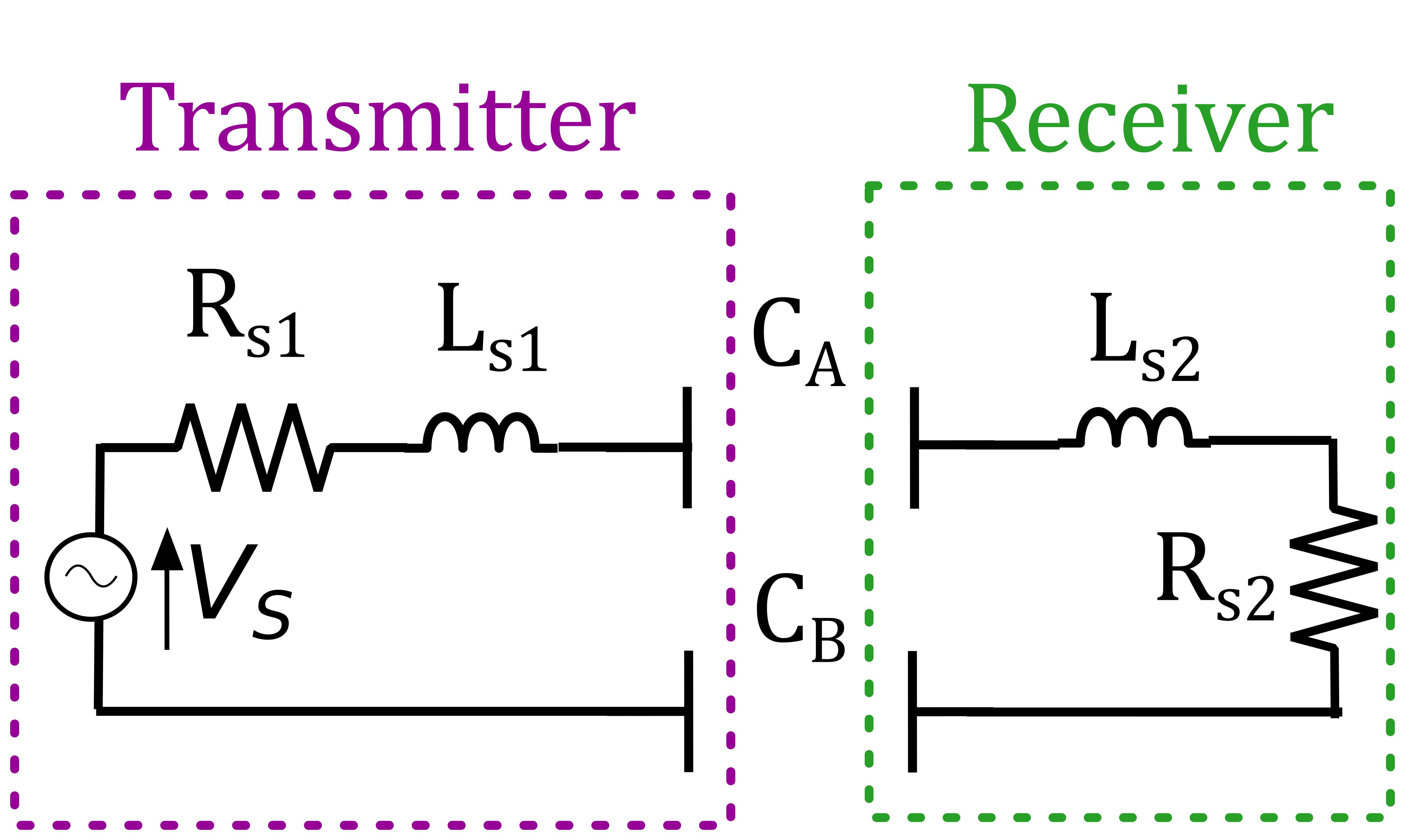
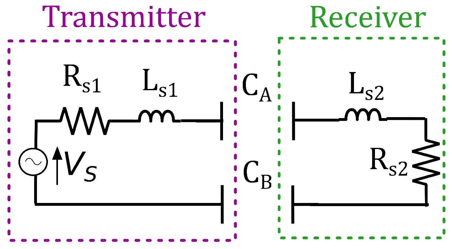
A general wireless power transfer link consists of a transmitter and a receiver. In a CPT system, the wireless link is realized by two conducting plates, at the transmitter and at the receiver side (Figure 1). These plates form two non-ideal, parallel facing capacitances and .
In order to enhance the wireless power transfer efficiency, a compensating circuit can be connected by adding an inductance to create a resonance circuit as well at the transmitter and the receiver side. In Figure 1, those inductances were placed in series, but also a parallel topology is possible. Thus, the transmitter of our general CPT system consists of an ideal time-harmonic voltage source at angular frequency , a series resistance , a series resonance inductance and the plates of the capacitances at the transmitter side. Analogously, the receiver consists of a series resistance , a series resonance inductance and the plates of the capacitances at the receiver side.
Obviously, Figure 1 is a simplification of a real CPT system, which will usually contain extra components (e.g., diode rectifier, H-bridge, power conditioner, ...). Nevertheless, we will use the simplified circuit in this study because (i) it is impossible to take into account all possible extra components that can be added, but, more importantly; (ii) it gives us the opportunity to focus on the effect of the WPT link itself, without the influences of external components. This allows a better understanding of the fundamentals of the WPT link, necessary for the design of a CPT system.
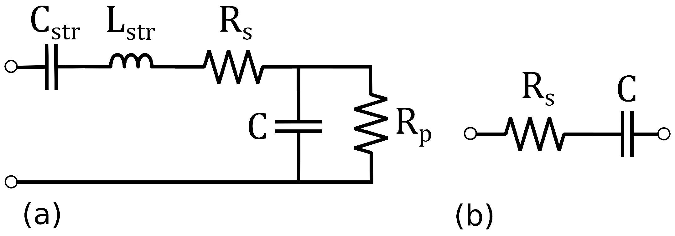
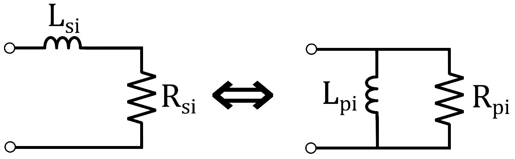
In order to correctly analyze this setup, the non-ideal capacitors have to be replaced by their equivalent circuit. A non-ideal capacitance consists of the following components (Figure 2a) [15,16,17]:
- A stray series capacitance , representing the terminal capacitance.
- A stray series inductance , caused by the leads and plates of the capacitor.
- The series resistance caused by the plates of and connections to the capacitor.
- The parallel resistance caused by the dielectric layer between the capacitor plates.
- The (ideal) capacitance C itself.
In practice, the series capacitance and inductance are negligible compared to the ideal capacitance C and the inductance of the compensating WPT network. Similarly, the resistance is large enough to justify neglecting it. This results in an equivalent circuit that is, for our application, a valid approximation for a non-ideal capacitor, consisting of the ideal capacitance C in series with the resistance (Figure 2b).
Replacing the non-ideal capacitors in Figure 1, we obtain the circuit from Figure 3a. This circuit has the disadvantage that the transmitter and receiver are part of the same circuit. Indeed, the transmitter and receiver share both the ideal capacitances and . This complicates the analysis of, e.g., a CPT system with one transmitter and multiple receivers. In order to be able to evaluate each receiver separately, it is beneficial to disconnect the transmitter and receiver circuit and introduce a coupling factor. Therefore, analogous to inductive power transfer, we construct the equivalent circuit (Figure 3b), with and the ideal capacitances of transmitter and receiver, respectively, and the mutual capacitance between and , as defined by [18]. The series resistances on the transmitter and receiver side, respectively, are and . The relationship between , , and on the one hand and , , , and , on the other hand, can be found in [19].
Analogous to inductive WPT, we introduce the capacitive coupling coefficient k (also named the electric coupling coefficient), defined as [18,19]:
We now consider the wireless link itself as a two-port network as indicated in Figure 3a. The wireless link is fully characterized by its impedance matrix , with elements (). Since the two-port network is linear and reciprocal (), the relationship between peak current and peak voltages (as defined in Figure 3a) at the two ports is given by:
Taking into account the equivalent circuit of Figure 3b, one can easily determine the coefficients of the impedance matrix Z of the two-port network:
The impedances connected to ports #1 and #2 are and , respectively (as indicated in Figure 3a).
By applying the conjugate image theory, we will determine in the next sections the optimal and to maximize the power transfer efficiency. We consider the impedance matrix and working frequency as given. In other words, given a fixed wireless link, what are the optimal impedances and to achieve maximum power transfer efficiency?
2.2. Conjugate Image Values for the Series Topology
We define the efficiency of the capacitive link as the ratio between the active output power delivered to a resistive load relative to the active input power provided by the source:
It was shown by Roberts [20] that applying the so-called conjugate-image configuration to a two-port network maximizes the power transfer efficiency from input port #1 to output port #2 and vice versa. We will apply this setup to determine the necessary network elements and to achieve maximum efficiency of the wireless link.
We want to stress that maximizing the efficiency of the power transfer does not correspond with maximizing the amount of transferred power to the load [21]. It can depend on the application whether the maximum efficiency or maximum power transfer solution is preferable. For example, for the wireless charging of biomedical implants, the maximum power configuration may be preferable, whereas for the wireless charging of electric vehicles, the maximum efficiency configuration is more appropriate [14,22]. In the next section, we will indicate the complex conjugate with a star: is the complex conjugate of Z.
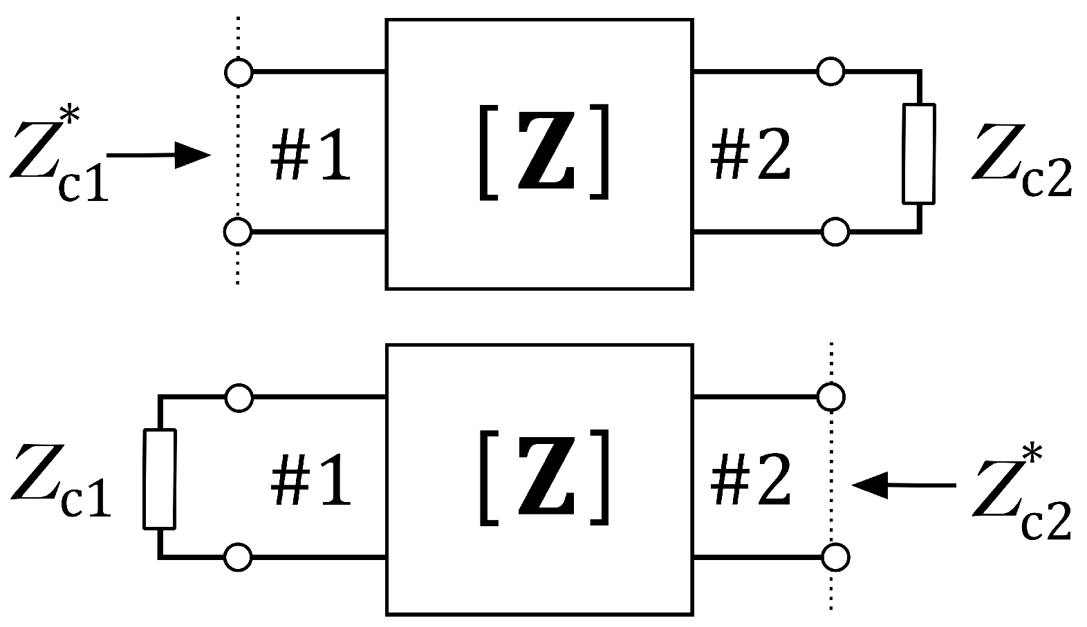
The conjugate image setup can be constructed by connecting specific impedances and to port #1 and #2, respectively [20,23]. It is said that the conjugate image configuration is achieved when the following conditions apply (Figure 4):
- If we terminate port #2 with a load , the impedance as seen into port #1 is .
- If we terminate port #1 with an impedance , the impedance as seen into port #2 is .
Written as a function of the coupling factor k, we obtain the expressions in Table 1.
In conclusion, the conjugate image theory teaches us that for maximizing the power transfer efficiency, the optimal values for the resistances and inductances in series, given a certain CPT link with impedance Z, are given by Equations (12), (13), (16) and (17).
In a general CPT system, the supply will be connected to port #1 of the two-port network, whereas the load will be connected to port #2. In that case, the resistance is redundant. It is only necessary if you want to maximize the efficiency in both directions. Indeed, the conjugate image setup not only maximizes the efficiency from port #1 (with the supply) to port #2 (with the load), but also from port #2 to port #1 if the supply and load are inverted. In other words, it allows choosing the ports at which you connect supply and load. Often, this design requirement is not imposed, and one can simply omit , which leads to a doubling of the efficiency and corresponds to the maximum efficiency configuration of the wireless power system [22].
2.3. Conjugate Image Values for the Parallel Topology
In the previous section, we calculated from the conjugate image theory the ideal impedance at both ports for the series configuration. We can now easily calculate the ideal values for the parallel topology by imposing the same impedance as shown by the equivalent circuit in Figure 5. By choosing the same parallel topology definition as Inagaki [13], we will, further in this work, be able to make a correct comparison for the application of the conjugate image theory between IPT and CPT wireless power transfer.
We can write:
from which we can derive ():
2.4. Lossless Approximation
The results obtained in the previous paragraph are rather complex. In order to improve our insight, we will, just as in [13], approximate the model for a lossless situation, i.e., . Later in this work, it will be experimentally demonstrated that this assumption is acceptable.
From Table 1, we can write
For the lossless approximation, this equation becomes:
Analogously, we obtain:
Notice that the above equation is the same as Equations (16) and (17). The expression for the inductance does not change for the lossless approximation.
An overview for the lossless approximation can be found in Table 2.
2.5. Comparison between CPT and IPT
Table 3 gives an overview of the resistive and reactive components of the compensation network for achieving maximum efficiency for CPT and IPT. The table is valid for both the series and parallel topology. The expressions for IPT were derived by Inagaki [13] and were validated for the lossless approximation. By defining the coupling function , which is a function of the coupling factor k, we obtain the same expressions for series and parallel topology. The coupling function is given by the values indicated in Table 4.
It is possible to write the values for the compensation network even more concisely than Table 3 by expressing them with the reactance:
for the inductance and capacitance, respectively. We obtain one formula for the resistive part of the conjugate image compensation network, valid for CPT and IPT, as well for the series and parallel topology:
is the reactance of the wireless link components, i.e., for CPT or for IPT. In addition, for the reactive part of the conjugate image compensation network, we obtain a single formula, valid for CPT and IPT, as well for the series as the parallel topology:
In the case of CPT, in Equation (29) is the reactance of the wireless link components and is the reactance of the compensation network. For IPT, in the above equation is the reactance of the wireless link components and is the reactance of the compensation network.
The introduction of the coupling function , as defined in Table 4, allows us to write the network elements to maximize the efficiency of the wireless power transfer in two elegant Equations (28) and (29). We will now discuss this coupling function for CPT and IPT, and thereby also compare the conjugate image theory between CPT and IPT. Notice that, since , the coupling function is only defined within this region.
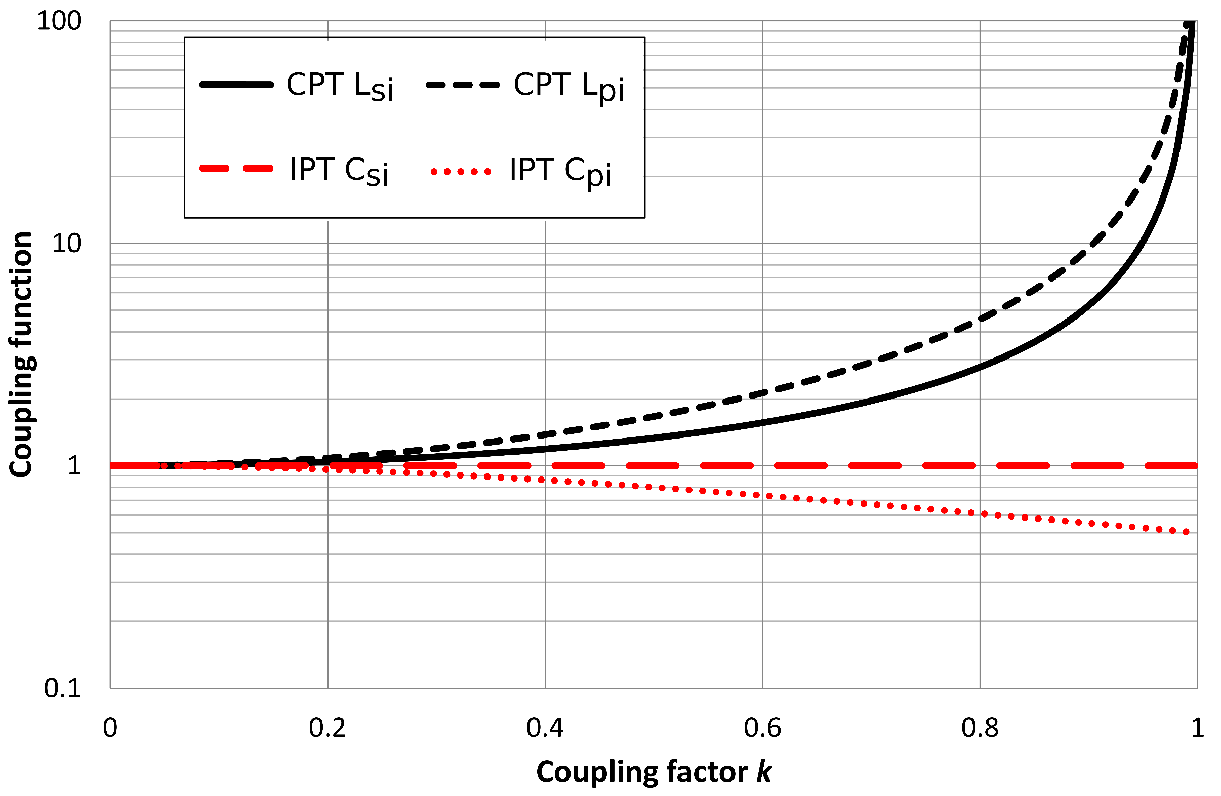
Figure 6 shows the coupling function as a function of k for and for CPT and IPT. The coupling function for the series resistance increases monotonically for higher coupling coefficients k. For low coupling (), its value for CPT is practically equal to its value for IPT. For very high coupling, rises very quickly for CPT, whereas for IPT, it converges to unity. Just as for , the coupling function for is also practically equal for CPT and IPT at low coupling (). Whereas for IPT, the function decreases monotonically, it rises again, quite strongly, for CPT. Regarding the resistive part of the compensation network, we can conclude that for low coupling, the values for CPT and IPT barely differ, whereas for high coupling, is low for IPT, but high for CPT. Notice that according to Equation (28), this corresponds with a low and for IPT, and a high and for CPT.
Figure 7 shows the coupling function as a function of k for the series and parallel reactive parts of the compensation network, for CPT and IPT systems. The coupling function for and increases monotonically for CPT at higher coupling coefficients k, whereas for , it decreases monotonically for IPT. The coupling function for is independent of k and remains constant at unity. For very low coupling (), the value for equals approximately unity in all four cases. For very high coupling, rises very quickly for CPT. The value for the parallel topology rises a bit faster, but the difference remains small. The situation is different for IPT: for higher coupling factors, remains at unity or goes to 0.5 for and , respectively. Regarding the reactive part of the compensation network, we can conclude that for low coupling, the values for CPT and IPT barely differ, whereas for high coupling, is high for CPT and low for IPT. Notice that according to Equation (29), this corresponds with a high inductance for CPT and a low capacitance for IPT.
According to Equations (26), (27) and (29), for all k corresponds to the natural resonance frequency of an uncoupled resonant circuit. Only the value for (IPT) corresponds to this natural frequency. All other optimal values do not agree with this natural frequency due to the coupling between the transmitter and receiver [24].
3. Validation
3.1. Setup
We construct a CPT system to illustrate the methodology of Section 2. We use four aluminum plates, each 200 mm × 300 mm × 1.2 mm, to construct the capacitances for the wireless power transfer link (Figure 1 and Figure 8) with values 462 pF ± 0.5 pF, 415 pF ± 0.5 pF, and 17 Ω ± 0.5 Ω. We use a plate of polyvinyl chloride (PVC) as material for the capacitances to create a dielectric gap of 2.5 mm between the metal plates. We apply a sinusoidal harmonic voltage of = V ± 0.05 V peak to peak at 300 kHz ± 0.5 Hz. We will use the same notation as in [19] and call the aluminum plates of the capacitors and at the transmitter side “A” and “B”, respectively. The plates at the receiver side of the capacitors and are named “a” and “b”, respectively. The capacitances between the different plates are named through their subscripts, e.g., is the capacitance between plate A and plate b. We measure the capacitance between the different plates at 300 kHz with an Agilent 4285A LCR meter (Keysight Technologies, Santa Rosa, CA, USA), as well as the series resistance of and . The results can be found in Table 5.
By measuring the open circuit voltage at the receiver side when applying the voltage source at the transmitter, we obtain the open circuit voltage . With the following equations:
which were derived by Huang and Hu [19], we are able to calculate , and . The coupling factor k is given by Equation (1). The results are summarized in Table 5. The corresponding Q-factor of and is 891 ± 34. We remark that a small margin of error in the determination of the capacitances leads to a relatively larger margin of error of e.g., the coupling factor k.
3.2. Series Topology
Given the values of Table 5, we can calculate the series resistance and the series inductance for the series topology. Since the values of the constructed capacitances are close to each other, Equations (22) and (23) lead to the same optimal value for the resistance and inductance at the transmitter and receiver side: = = kΩ ± 0.88 kΩ and = = mH ± 0.5 mH.
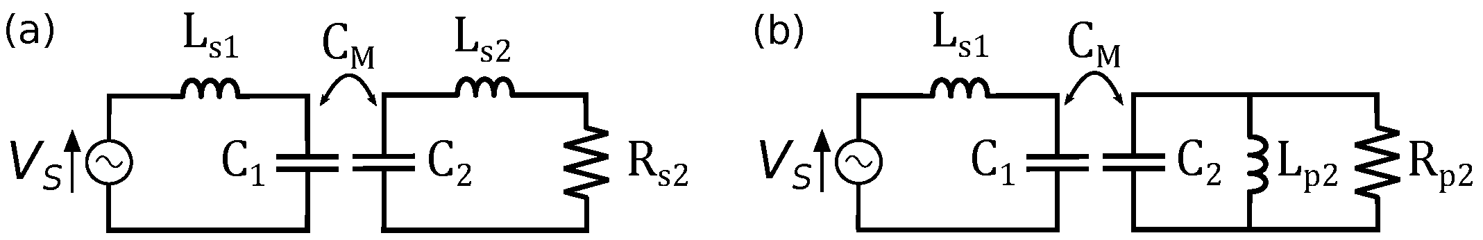
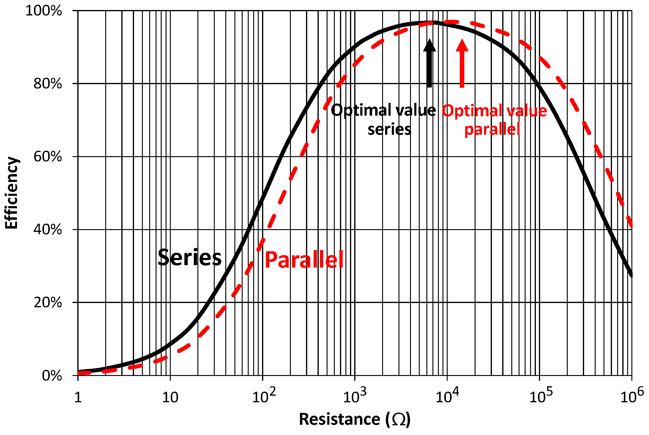
Figure 9a shows the series topology. Notice that we have omitted to obtain the maximum efficiency configuration of the CPT link as mentioned above. Figure 10 shows the efficiency at 300 kHz, as defined by Equation (7), as a function of when = = mH. These results take into account the series resistance of the capacitors and inductors and were acquired with the circuit simulator TINA-TI® (Texas Instruments, Dallas, TX, USA). The results confirm that the maximum occurs at = kΩ, from which we can conclude that our equations to determine the optimal series resistance for maximum efficiency are valid. Notice that the resistance region for an optimal efficiency is very broad, allowing a sizable range of loads for any practical application.
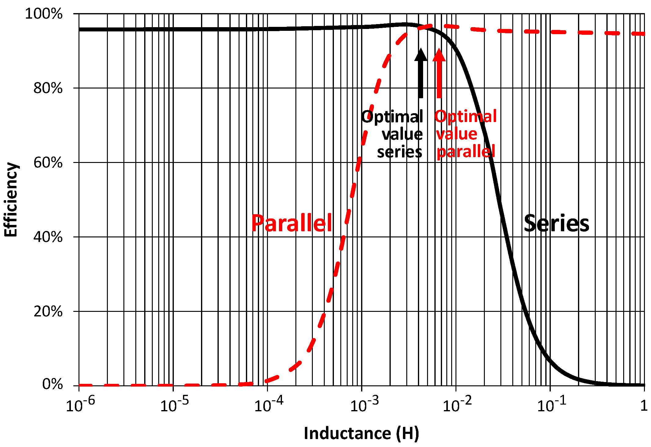
We can do the same analysis for the inductance. Figure 11 shows the efficiency as function of when = mH and = kΩ. The results confirm that the maximum occurs at = mH, from which we can conclude that our equations to determine the optimal series inductance for maximum efficiency are valid. We again notice that the region for an optimal efficiency is very broad.
3.3. Parallel Topology
We repeat the same analysis as above, but now for a parallel circuit instead of a series circuit at the receiver side (Figure 9b). Notice that a parallel topology at the transmitter side, as defined by Figure 5, is meaningless to obtain the maximum efficiency. Given the values of Table 5, we can calculate from Equations (24) and (25) the optimal resistance and inductance. We obtain = kΩ ± 1.7 kΩ and = mH ± 0.9 mH. Figure 10 and Figure 11 show the influence of varying and , respectively, when the other components have their optimal value. The same conclusions as the series topology can be drawn.
The theoretical maximum achievable efficiency of the wireless link itself, characterized by its impedance matrix Z, can be analytically calculated using the values of Table 5. This efficiency is given by [25]:
with defined as:
Since and are small, we find for the wireless link itself an almost ideal power transfer efficiency of = 99.9%. If we take the series resistance of the inductors into account, we obtain the same maximum value as obtained by the simulations, i.e., 96.7%.
4. Discussion
The conjugate image solution allows us to determine the optimal compensation network (i.e., the optimal impedance at the ports) to obtain the maximum power transfer efficiency of the WPT system. We have shown that this optimal impedance is dependent on the coupling factor k. If k is constant, the optimal impedance obviously does not change. However, for certain applications such as moving electric vehicles [26], automated guided vehicles [27] and a computer mouse [28], this coupling factor is variable in time. In that case, one has to allow that an ideal compensation network is not present all of the time, leading to non optimal transfer efficiencies. A possible solution is to adapt the matching network according to the changing coupling factor [29]. In view of this, we will discuss the results obtained in the above calculations for the lossless approximation as a function of the coupling factor k and study the sensitivity on k.
We start by discussing the resistive part. The higher the k, the higher the optimal value for . For realistic values of a CPT system, the optimal value of can vary over several orders of magnitude. In contrast to , the variability for is much smaller for varying coupling factors. For very high () or very low () coupling factors, the optimal value for is high, whereas for values in between, the value is relatively low and fairly constant. There exists a broad range of coupling factors () where marginal or no adaptation is necessary for varying coupling regarding . The ratio of to is approximately for small k.
For low coupling factors (), the inductive part of the compensation network, i.e., the inductance or , remains more or less constant and relatively small. For higher k, the optimal inductance values rise quickly, certainly for . This implies that at low coupling, no adaptation for the reactive part of the compensation network is necessary, even if the coupling factor k is varying strongly, as long as the coupling remains low (). For high coupling, the variability is much higher, resulting in a significant decrease of efficiency for varying coupling factors. At low coupling, and are practically equal. At higher coupling, the optimal value of rises a bit faster than , but they remain within the same order of magnitude.
5. Conclusions
The conjugate image theory is applied for determining the optimal compensation network at the input and output port of a CPT link as a function of the properties of the wireless power transfer link. Expressions to obtain maximum efficiency for series and parallel topology are derived, leading to a set of closed expressions. By introducing a new concept, the coupling function, we were able to describe the compensation network of a CPT and IPT system in only two compact equations, valid for the series and parallel topology as well. This allows for gaining a deeper insight into the fundamentals of the WPT link, necessary for the design of an efficient WPT system.
Acknowledgments
This work was supported by the iMinds-MoniCow project, co-funded by iMinds, a research institute founded by the Flemish Government in 2004, and the involved companies and institutions.
Author Contributions
Ben Minnaert initiated the study, performed the calculations and conducted the experiments; Nobby Stevens provided the general supervision of the calculations and experiments; Ben Minnaert wrote the manuscript; Nobby Stevens revised and commented on the manuscript.
Conflicts of Interest
The authors declare no conflict of interest.
Abbreviations
The following abbreviations are used in this manuscript:
| CPT | Capacitive power transfer |
| IPT | Inductive power transfer |
| WPT | Wireless power transfer |
References
- Brown, W.C. The history of power transmission by radio waves. IEEE Trans. Microw. Theory Tech. 1984, 32, 1230–1242. [Google Scholar] [CrossRef]
- Roes, M.G.; Duarte, J.L.; Hendrix, M.A.; Lomonova, E.A. Acoustic energy transfer: A review. IEEE Trans. Ind. Electron. 2013, 60, 242–248. [Google Scholar] [CrossRef]
- Lu, X.; Wang, P.; Niyato, D.; Kim, D.I.; Han, Z. Wireless charging technologies: Fundamentals, standards, and network applications. IEEE Commun. Surv. Tutor. 2015, 18, 1413–1452. [Google Scholar] [CrossRef]
- Kumar, A.; Pervaiz, S.; Chang, C.K.; Korhummel, S.; Popovic, Z.; Afridi, K.K. Investigation of power transfer density enhancement in large air-gap capacitive wireless power transfer systems. In Proceedings of the IEEE Wireless Power Transfer Conference, Boulder, CO, USA, 13–15 May 2015; pp. 1–4.
- Mi, C. High power capacitive power transfer for electric vehicle charging applications. In Proceedings of the 6th IEEE International Conference on Power Electronics Systems and Applications (PESA), Hong Kong, China, 15–17 December 2015; pp. 1–4.
- Hanazawa, M.; Ohira, T. Power transfer for a running automobile. In Proceedings of the IEEE MTT-S International Microwave Workshop Series on Innovative Wireless Power Transmission: Technologies, Systems, and Applications (IMWS 2011), Kyoto, Japan, 12–13 May 2011; pp. 77–80.
- Funato, H.; Kobayashi, H.; Kitabayashi, T. Analysis of transfer power of capacitive power transfer system. In Proceedings of the IEEE 10th International Conference on Power Electronics and Drive Systems (PEDS), Kitakyushu, Japan, 22–25 April 2013; pp. 1015–1020.
- Huang, L.; Hu, P.; Swain, A.; Su, Y. Z. Impedance compensation for wireless power transfer based on electric field coupling. IEEE Trans. Power Electron. 2016, 31, 7556–7563. [Google Scholar] [CrossRef]
- Komaru, T.; Akita, H. Positional characteristics of capacitive power transfer as a resonance coupling system. In Proceedings of the IEEE Wireless Power Transfer Conference, Perugia, Italy, 15–16 May 2013; pp. 218–221.
- Liu, C.; Hu, A.P.; Budhia, M. A generalized coupling model for capacitive power transfer systems. In Proceedings of the IECON 2010—36th Annual Conference on IEEE Industrial Electronics Society, Glendale, AZ, USA, 7–10 November 2010; pp. 274–279.
- Liu, C.; Hu, A.P.; Nair, N.K.C. Coupling study of a rotary Capacitive Power Transfer system. In Proceedings of the 2009 IEEE International Conference on Industrial Technology, Churchill, Victoria, Australia, 10–13 February 2009; pp. 1–6.
- Xia, C.; Zhou, Y.; Zhang, J.; Li, C. Comparison of power transfer characteristics between CPT and IPT system and mutual inductance optimization for IPT system. J. Comput. 2012, 7, 2734–2741. [Google Scholar] [CrossRef]
- Inagaki, N. Theory of image impedance matching for inductively coupled power transfer systems. IEEE Trans. Microw. Theory Tech. 2014, 62, 901–908. [Google Scholar] [CrossRef]
- Monti, G.; Costanzo, A.; Mastri, F.; Mongiardo, M. Optimal design of a wireless power transfer link using parallel and series resonators. Wirel. Power Transf. 2016, 3, 105–116. [Google Scholar] [CrossRef]
- Malek, H.; Dadras, S.; Chen, Y. Fractional order ESR modeling of electrolytic capacitor and fractional order failure prediction with application to predictive maintenance. IET Power Electron. 2016, 9, 1608–1613. [Google Scholar] [CrossRef]
- Whitaker, J.C. AC Power Systems Handbook, 2nd ed.; Chemical Rubber Company (CRC) Press: Boca Raton, FL, USA, 2002; pp. 53–54. [Google Scholar]
- Bowick, C. RF Circuit Design Howard, 3rd ed.; Elsevier: Burlington, VT, USA, 1982; pp. 12–13. [Google Scholar]
- Hong, J.S.G.; Lancaster, M.J. Microstrip Filters for RF/Microwave Applications, 1st ed.; John Wiley & Sons: New York, NY, USA, 2001; pp. 235–253. [Google Scholar]
- Huang, L.; Hu, A.P. Defining the mutual coupling of capacitive power transfer for wireless power transfer. Electron. Lett. 2015, 51, 1806–1807. [Google Scholar] [CrossRef]
- Roberts, S. Conjugate-image impedances. Proc. IRE 1946, 34, 198–204. [Google Scholar] [CrossRef]
- Dionigi, M.; Mongiardo, M.; Perfetti, R. Rigorous network and full-wave electromagnetic modeling of wireless power transfer links. IEEE Trans. Microw. Theory Tech. 2015, 63, 65–75. [Google Scholar] [CrossRef]
- Dionigi, M.; Mongiardo, M.; Monti, G.; Perfetti, R. Modelling of wireless power transfer links based on capacitive coupling. Int. J. Numer. Model. 2016. [Google Scholar] [CrossRef]
- Costanzo, A.; Dionigi, M.; Masotti, D.; Mongiardo, M.; Monti, G.; Tarricone, L.; Sorrentino, R. Electromagnetic energy harvesting and wireless power transmission: A unified approach. Proc. IEEE 2014, 102, 1692–1711. [Google Scholar] [CrossRef]
- Aditya, K.; Youssef, M.; Williamson, S.S. Analysis of series-parallel resonant inductive coupling circuit using the two-port network theory. In Proceedings of the IEEE IECON 2015—41st Annual Conference of the Industrial Electronics Society, Yokohama, Japan, 9–12 November 2015; pp. 005402–005407.
- Ohira, T. Extended K-Q product formulas for capacitive-and inductive-coupling wireless power transfer schemes. IEICE Electron. Express 2014, 11. [Google Scholar] [CrossRef]
- Bavastro, D.; Canova, A.; Cirimele, V.; Freschi, F.; Giaccone, L.; Guglielmi, P.; Repetto, M. Design of wireless power transmission for a charge while driving system. IEEE Trans. Magn. 2014, 50, 965–968. [Google Scholar] [CrossRef]
- Pacini, A.; Mastri, F.; Trevisan, R.; Masotti, D.; Costanzo, A. Geometry optimization of sliding inductive links for position-independent wireless power transfer. In Proceedings of the IEEE Microwave Theory and Techniques Society (MTT-S) International Microwave Symposium (IMS), San Francisco, CA, USA, 22–27 May 2016; pp. 1–4.
- Thoen, B.; Wielandt, S.; De Baere, J.; Goemaere, J.P.; De Strycker, L.; Stevens, N. Design of an inductively coupled wireless power system for moving receivers. In Proceedings of the IEEE Wireless Power Transfer Conference, Jeju City, Korea, 8–9 May 2014; pp. 48–51.
- Waters, B.H.; Sample, A.P.; Smith, J.R. Adaptive impedance matching for magnetically coupled resonators. In Proceedings of the 32nd Progress in Electromagnetics Research Symposium (PIERS), Moscow, Russia, 19–23 August 2012; pp. 694–701.
Figure 1.
An overview of a general capacitive power transfer (CPT) system.

Figure 2.
(a) The equivalent circuit of a non-ideal capacitance; and (b) a valid approximation for the equivalent circuit of a non-ideal capacitance.
Figure 2.
(a) The equivalent circuit of a non-ideal capacitance; and (b) a valid approximation for the equivalent circuit of a non-ideal capacitance.

Figure 3.
(a) A CPT system with the series topology. is the impedance matrix of the wireless link. and are the external impedances connected to port #1 and port #2, respectively, of the two-port network formed by the wireless link; and (b) equivalent circuit for the capacitive wireless link where the transmitter and receiver are separated into two coupled circuits.
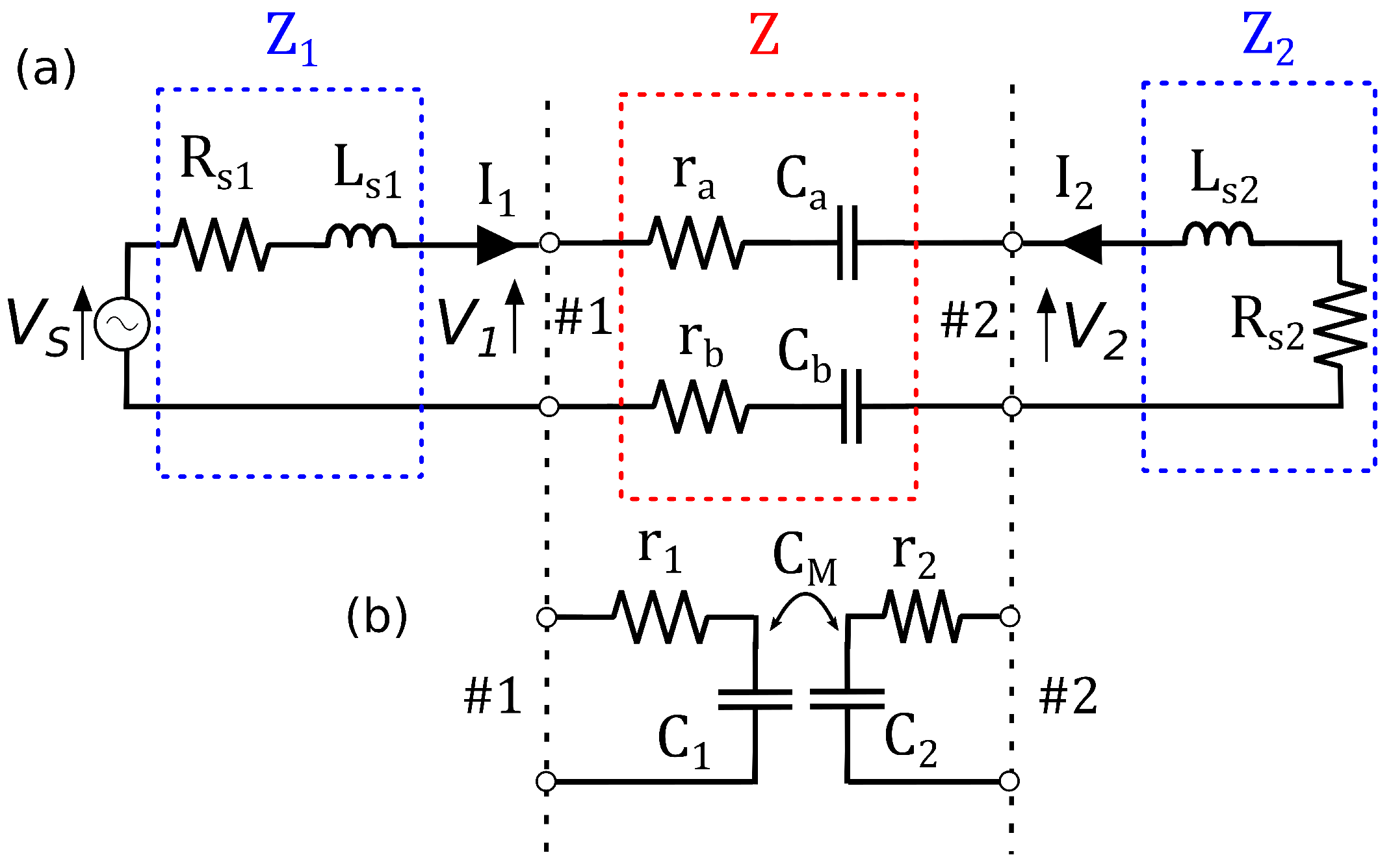
Figure 4.
In the conjugate image configuration, ports #1 and #2 of a two-port network are connected to and , respectively.
Figure 4.
In the conjugate image configuration, ports #1 and #2 of a two-port network are connected to and , respectively.

Figure 5.
We define and () such that the two given circuits are equivalent to each other.

Figure 6.
The coupling function as a function of the coupling factor k for the resistive parts of the compensation network for CPT and IPT, as well for the series as for the parallel topology.
Figure 6.
The coupling function as a function of the coupling factor k for the resistive parts of the compensation network for CPT and IPT, as well for the series as for the parallel topology.

Figure 7.
The coupling function as a function of the coupling factor k for the reactive parts of the compensation network for CPT and IPT, as well for series and parallel topology.
Figure 7.
The coupling function as a function of the coupling factor k for the reactive parts of the compensation network for CPT and IPT, as well for series and parallel topology.

Figure 8.
A picture of the setup: four aluminum plates with polyvinyl chloride (PVC) as dielectric material are used to create the capacitances and .
Figure 8.
A picture of the setup: four aluminum plates with polyvinyl chloride (PVC) as dielectric material are used to create the capacitances and .

Figure 9.
Circuit representation of the CPT setup. The series resistances of the capacitors and inductors are not shown. (a) The series topology; (b) the parallel topology.
Figure 9.
Circuit representation of the CPT setup. The series resistances of the capacitors and inductors are not shown. (a) The series topology; (b) the parallel topology.

Figure 10.
The power transfer efficiency as a function of the load for the series and parallel topology. The calculated optimal value for each topology is indicated with an arrow.
Figure 10.
The power transfer efficiency as a function of the load for the series and parallel topology. The calculated optimal value for each topology is indicated with an arrow.

Figure 11.
The power transfer efficiency as function of the inductance at the receiver side for the series and parallel topology. The calculated optimal value for each topology is indicated with an arrow.
Figure 11.
The power transfer efficiency as function of the inductance at the receiver side for the series and parallel topology. The calculated optimal value for each topology is indicated with an arrow.


Table 1.
The conjugate image resistances and inductances for the series and parallel topology, with or .
| R | L | |
|---|---|---|
| Series | ||
| Parallel |
Table 2.
The conjugate image resistances and inductances for the series and parallel topology for the lossless approximation, with .
| R | L | |
|---|---|---|
| Series | ||
| Parallel |
Table 3.
Overview of the resistive and reactive components of the compensation network for achieving maximum efficiency for CPT and IPT, as well for series and parallel topology, with for CPT and for IPT. Notice that if we introduce the coupling function as defined in Table 4, the expressions for series and parallel topology are equal to each other.
| CPT | IPT | |
|---|---|---|
| CPT | IPT | |
|---|---|---|
| k | ||
| 1 | ||
| Quantity | Value | Quantity | Value |
|---|---|---|---|
| 462 pF ± 0.5 pF | 17 Ω ± 0.5 Ω | ||
| 415 pF ± 0.5 pF | 17 Ω ± 0.5 Ω | ||
| 2.7 pF ± 0.5 pF | 220 pF ± 1.7 pF | ||
| 2.7 pF ± 0.5 pF | 220 pF ± 1.7 pF | ||
| 2.4 pF ± 0.5 pF | 20.0 V ± 0.05 V | ||
| 2.3 pF ± 0.5 pF | 16.4 V± 0.05 V | ||
| k | 82.9% ± 1.8% | 182 pF ± 2.8 pF |
© 2017 by the authors; licensee MDPI, Basel, Switzerland. This article is an open access article distributed under the terms and conditions of the Creative Commons Attribution (CC-BY) license (http://creativecommons.org/licenses/by/4.0/).
Share and Cite
MDPI and ACS Style
Minnaert, B.; Stevens, N. Conjugate Image Theory Applied on Capacitive Wireless Power Transfer. Energies 2017, 10, 46. https://doi.org/10.3390/en10010046
AMA Style
Minnaert B, Stevens N. Conjugate Image Theory Applied on Capacitive Wireless Power Transfer. Energies. 2017; 10(1):46. https://doi.org/10.3390/en10010046
Chicago/Turabian StyleMinnaert, Ben, and Nobby Stevens. 2017. "Conjugate Image Theory Applied on Capacitive Wireless Power Transfer" Energies 10, no. 1: 46. https://doi.org/10.3390/en10010046
Note that from the first issue of 2016, this journal uses article numbers instead of page numbers. See further details here.