A Soft Sensor-Based Fault-Tolerant Control on the Air Fuel Ratio of Spark-Ignition Engines

Abstract

The air/fuel ratio (AFR) regulation for spark-ignition (SI) engines has been an essential and challenging control problem for engineers in the automotive industry. The feed-forward and feedback scheme has been investigated in both academic research and industrial application. The aging effect can often cause an AFR sensor fault in the feedback loop, and the AFR control performance will degrade consequently. In this research, a new control scheme on AFR with fault-tolerance is proposed by using an artificial neural network model based on fault detection and compensation, which can provide the satisfactory AFR regulation performance at the stoichiometric value for the combustion process, given a certain level of misreading of the AFR sensor.

1. Introduction

The primary objective of modern engine control systems is to maintain the combustion process at the low-emission condition while satisfying the requirements on higher efficiency, performance, and reliability [1]. It needs not only design efforts on engine operating conditions, but also the reliable methods to measure system states, which is needed for the implementation of control strategies. However, the high-performance control of the dynamics of internal combustion engines is difficult to achieve due to unpredictable changes of load. For example, in order to obtain the desired balance between power output and fuel consumption in spark-ignition (SI) engines, the air/fuel ratio (AFR) must be maintained at the stoichiometric value (14.7) for both steady state and transient operation. The efficiency of three-way catalysts (TWC) is significantly influenced by the air fuel ratio. It has been reported that only the stoichiometric value provides its optimal operating condition. If AFR is 1% lower than 14.7, the emissions level of carbon monoxide (CO) and hydrocarbons (HC) can increase significantly. If AFR is 1% higher than 14.7, up to 50% more NO_x will be produced [1,2]. In addition, the dynamics of the air manifold and fuel injection of internal combustion engines are very fast, severely nonlinear, and constraints are imposed on the states and inputs [3,4,5,6]. Therefore, AFR regulation has been a popular topic in areas over automotive industry and theoretical research.

The most popular control method of automotive engineering is the model-free methodology to design engine control units (ECU). A tremendous number of cycles need to be run in the engine test-bed to acquire sufficient data to fill in the lookup table, which takes a significant amount of time for calibration. For each operating condition, numerous measurement variables are needed to be performed and averaged to show the desirable robustness. In addition, the designing of an ECU should be considered for the case of aging effects, because the engine performance could be degraded from aging effects and component faults. A static table with fixed control data is not sufficient to meet the requirement of government law on emissions and specified performance. With the development of computational power with micro-controllers, advanced model-based approaches for the design and analysis of engine controls have been reported to improve the current results by the traditional method [1]. Recently, a signal spectral analysis method on a universal exhaust gas oxygen (UEGO) sensor was proposed by Cavina et al. [7] to control the AFR for an individual engine cylinder, and its result show that the error of the lambda regulation can be controlled within a bound of 0.01. Alfieri et al. [8] implemented a robust control design method into an engine control system, and feed-forward controllers were investigated for disturbance dynamics compensation. Ebrahimi et al. [9] designed an improved new proportional-integral-derivative (PID) controller for SI engines, which is parameter-varying filtered. The innovative control approach on automotive engine systems by Khiar et al. [10] and Yildiz et al. [11] combined fuzzy control and adaptive control. It can be seen that the control performance has been improved by these advanced methods. However, as mentioned, the advanced strategies on control require the reliable measurement on engine operating states. In this case, the impact of engine aging effects and sensor faults on control performance must be considered during control system design. For example, sensors and actuators are usually included in the engine control loop, so faults can result in a significant change on controlled dynamics. Therefore, it increases in emissions and causes severe air pollution. The on-board diagnosis (OBD) module is compulsory in modern engine management system. Its purpose is for early detection and repair of malfunctions that can result in fewer emissions. Hence, early repair of minor problems may prevent more significant and more expensive engine problems that could develop if undetected. Furthermore, a fault-tolerant control scheme (FTCS) is needed, which can tolerate system faults by maintaining suitable operating conditions.

According to the difference on design philosophy, FTCSs have developed into two groups, namely, passive FTCSs (PFTCS) and active FTCSs (AFTCS). The PFTCS controller is designed to possess a certain robust level for given specific presumed faults. The model of these faults, such as types and boundaries, are assumed to be known during the design, and then they can be considered during controller synthesis. Controller parameters in this case are fixed values after the design phase, and the controller can only deal with these faults with expected types and boundaries. Based on the concept of higher-order sliding mode control, Ali proposed a control strategy with passive fault-tolerance for the air path dynamics control of a diesel engine. Actuator fault conditions are considered during controller design, and computer simulation results of good control performance can be obtained under pre-specified faults conditions [12]. Robust control has been implemented by Tao for aircraft engines subject to faults in sensors and/or actuators in discontinuous patterns. He adopted the linear matrix inequality to derive sufficient conditions for achieving fault tolerance from linear models and ensuring a control performance index [13].

AFTCS typically consists of two parts—a fault detection and isolation tool (FDI) that detect the fault with the utilization of physical (additional hardware sensors) or analytical (soft sensors) redundancy. The data by fault analysis is delivered to a mechanism that can reconfigure the control data. The self-reconfigured controller can then maintain the specified control performance with faults. For the water management of a fuel cell, Lebreton et al. [14] developed an active fault-tolerant control that was tested on a polymer electrolyte membrane fuel cell system. The artificial neural network-based fault-tolerance system showed very promising results. A comprehensive research study between active and passive approaches for fault-tolerant control/regulation systems can be found in Jiang and Xu’s work [15].

In this paper, a soft sensor based fault-tolerant control strategy for the fuel injection system of a SI engine is proposed, which can deal with the AFR sensor fault promptly and keep a satisfactory performance given a sensor misreading. The remainder of this paper is organized as follows. In Section 2, a SI engine model based on first principles is introduced, from which the input and output data of a SI engine are defined. Engine dynamics modeling by neural networks for both control and fault tolerance are described in Section 3. Section 4 shows the configuration of FTCS and its implementation on AFR regulation. The developed FTCS is tested by simulation, and results are shown as well. Finally, the conclusions are drawn in Section 5.

2. Spark-Ignition Engine Dynamics

The engine model adopted in this research is the mean value engine model (MVEM) developed by Hendricks et al. [16], which is a widely-used benchmark for engine modeling and control. The platform which has been selected for this MVEM is the well-known MATLAB/SIMULINK (Version 7.1, MathWorks, Natick, MA, USA). The three distinct systems of this model are the fuel injection, manifold filling, and the crankshaft speed dynamic subsystems; those systems are modeled independently. Since this MVEM can achieve a steady state accuracy of about ±2% over the entire operating range of the engine, it is extremely useful for the validation of control strategies using simulation. A full description of the MVEM can be found in [16].

2.1. Manifold Air-Filling Dynamics

There are usually two non-linear differential equations that can be used to analyse the intake-filling dynamics, one for the manifold pressure and the other for the manifold temperature. The derivation is based on the air mass conservation inside the intake manifold. The manifold pressure is mainly related to the air mass flow past the throttle plate, the air mass flow into the intake port, the exhaust gas re-circulation (EGR) mass flow, the EGR temperature and the manifold temperature. It is described as:

$${\dot{p}}_i=\frac{\mathsf{\kappa }\mathrm{R}}{V_i}\left(-{\dot{m}}_{ap}{T}_i+{\dot{m}}_{at}{T}_a+{\dot{m}}_{EGR}{T}_{EGR}\right)$$

(1)

where $p_i$ is the absolute manifold pressure ($\mathrm{N}/{\mathrm{m}}^2$), ${\dot{m}}_{at}$ is the air mass flow past throttle plate (kg/s), $T_i$ is the intake manifold temperature (K), ${\dot{m}}_{ap}$ is the air mass flow into intake port (kg/s), $T_a$ is the ambient temperature (K), ${\dot{m}}_{EGR}$ is the EGR mass flow (kg/s), $T_{EGR}$ is the EGR temperature (K), $V_i$ is the manifold port passage volume (${\mathrm{m}}^3$), R is the gas constant ($2.87\times {10}^{-5}$), and $\mathsf{\kappa }$ is ratio of the specific heats equal to 1.4 for air.

Equation (2) describes the dynamics of manifold temperature:

$${\dot{T}}_i=\frac{\mathrm{R}{T}_i}{p_i{V}_i}\left[-{\dot{m}}_{ap}\left(\mathsf{\kappa }-1\right)T_i+{\dot{m}}_{at}\left(\mathsf{\kappa }{T}_a-T_i\right)+{\dot{m}}_{EGR}\left(\mathsf{\kappa }{T}_{EGR}-T_i\right)\right]$$

(2)

Equations (1) and (2) can be realised by MATLAB/SIMULINK. The air mass flow dynamics in the intake manifold can be described as follows: The air mass flow past throttle plate ${\dot{m}}_{at}$ is related with the throttle position and the manifold pressure. The air mass flow into the intake port ${\dot{m}}_{ap}$ is represented by a well-known speed-density equation:

$${\dot{m}}_{at}\left(u,p_i\right)={\dot{m}}_{at1}\frac{p_a}{\sqrt{T_a}}{\mathsf{\beta }}_1\left(u\right){\mathsf{\beta }}_2\left(p_r\right)+m_{at0}$$

(3)

$${\dot{m}}_{ap}\left(n,p_i\right)=\frac{V_d}{120\mathrm{R}{T}_i}\left({\mathsf{\eta }}_i{p}_i\right)n$$

(4)

where:

$${\mathsf{\beta }}_1\left(u\right)=1-cos\left(u\right)-\frac{u_0^2}{2!}$$

(5)

$${\mathsf{\beta }}_2\left(p_r\right)=\{\begin{array}{ccc}\sqrt{1-{\left(\frac{p_r-p_c}{1-p_c}\right)}^2}& \mathrm{if}& p_r\ge p_c\\ 1& \mathrm{if}& p_r<p_c\end{array}$$

(6)

$$p_r=\frac{p_i}{p_a}$$

(7)

$m_{at0}$, $m_{at1}$, $u_0$, and $p_c$ are engine constants that can be identified during model validation in the engine test-bed. $u$ is the throttle position in degrees, $V_d$ is the engine displacement in liters, $n$ is the crankshaft speed in rpm. Additionally, instead of directly modelling the volumetric efficiency ${\mathsf{\eta }}_i$, it is easier to generate the quantity ${\mathsf{\eta }}_i\times p_i$ which is called normalised air charge. The normalised air charge can be obtained by the steady state engine test and is approximated with the polynomial Equation (8):

$${\mathsf{\eta }}_i{p}_i=s_i\left(n\right)p_i+y_i\left(n\right)$$

(8)

where $s_i\left(n\right)$ and $y_i\left(n\right)$ are positive, weak functions of the crankshaft speed, and $y_i\ll s_i$.

2.2. Engine Speed Dynamics

The engine speed $n$, also called crankshaft speed, is derived based on the conservation of the rotational energy on the crankshaft. Its dynamics is given as follows:

$$\dot{n}=-\frac{1}{In}\left[P_f\left(p_i,n\right)+P_p\left(p_i,n\right)+P_b\left(n\right)\right]+\frac{1}{In}{H}_u{\mathsf{\eta }}_i\left(p_i,n,\mathsf{\lambda }\right){\dot{m}}_f\left(t-{\Delta \mathsf{\tau }}_d\right)$$

(9)

Both the friction power $P_f$ (kW) and the pumping power $P_p$ (kW) are related with the manifold pressure $p_i$ and the crankshaft speed n. The load power $P_b$ (kW) is a function of the crankshaft speed n only. The indicated efficiency ${\mathsf{\eta }}_i$ is a function of the manifold pressure $p_i$, the crankshaft speed n and the air fuel ratio λ. $I$ is the crankshaft load inertia in kg$\cdot {\mathrm{m}}^2$, $H_u$ is the fuel lower heating value in kJ/kg, ${\Delta \mathsf{\tau }}_d$ is the injection torque delay time in seconds, and ${\dot{m}}_f$ is the engine port fuel mass flow in kg/s.

2.3. Fuel Injection Dynamics

It has been found that the fuel jet from the injector can be characterised into two portions. One portion mixes with the air stream and enters the cylinder directly; the other portion deposits as fuel film on the surfaces of the intake system components, and mixes with the air stream through the re-entrainment/evaporation process during subsequent engine cycles. This is known as wall-wetting.

According to Hendrick et al.’s [16] identification experiments with SI engines, the fuel flow dynamics could be described via the following equations:

$${\ddot{m}}_{ff}=\frac{1}{{\mathsf{\tau }}_f}\left(-{\dot{m}}_{ff}+X_f{\dot{m}}_{fi}\right)$$

(10)

$${\dot{m}}_{fv}=\left(1-X_f\right){\dot{m}}_{fi}$$

(11)

$${\dot{m}}_f={\dot{m}}_{fv}+{\dot{m}}_{ff}$$

(12)

where the model is based on keeping track of the fuel mass flow. ${\dot{m}}_{ff}$ is the fuel film mass flow, ${\dot{m}}_{fv}$ is the fuel vapor mass flow, ${\dot{m}}_{fi}$ is the injected fuel mass flow, and their units are all in kg/s. The parameters in the model are the time constant for fuel evaporation, ${\mathsf{\tau }}_f$, and the proportion of the fuel which is deposited on the intake manifold or close to the intake valves, $X_f$. These parameters are operating point dependently and, thus, the model is nonlinear in spite of its linear form. The MVEM was provided by Elbert Hendrick, and it has been validated using the real-time data acquired from the engine test-bed that was equipped with a Ford 1.6 L engine (Ford, Dearborn, MI, USA). The parameters for this model could be expressed approximately in terms of the states of the model as:

$${\mathsf{\tau }}_f\left(p_i,n\right)=1.35\left(-0.672n+1.68\right){\left(p_i-0.825\right)}^2+\left(-0.05n+0.15\right)+0.56$$

(13)

$$X_f\left(p_i,n\right)=-0.277p_i-0.055n+0.68$$

(14)

2.4. Mean Value Engine Model under Air/Fuel Ratio Measurement Delay

The AFR $\mathsf{\lambda }$ could be calculated using Equation (15):

$$\mathsf{\lambda }=\frac{{\dot{m}}_{ap}}{{\dot{m}}_f}$$

(15)

Nowadays, in the practical application of the automotive industry, oxygen sensors are used in the fuel injection system. They determine if the AFR exiting a gas-combustion engine is rich (with unburnt fuel vapour) or lean (with excess oxygen), then, a closed-loop feedback controller, such as a proportional-integral (PI) controller, adjusts the fuel injection rate $m_{fi}$ according to real-time sensor data rather than operating with an open-loop fuel map. Therefore, the time delay of injection systems should also be considered. Manzie et al. [17,18] showed there are three causes of time delay for injection systems: the two engine cycle delays between the injection fuel and the expulsion from the exhaust valves, the propagation delay for the exhaust gases to reach the oxygen sensor, and the sensor output delay. It has been found that the engine speed has more influence on these delays than the manifold pressure. Therefore, the following equation can be used to represent the delays of injection system $t_d$:

$$t_d=0.045+\frac{10\mathsf{\pi }}{n}$$

(16)

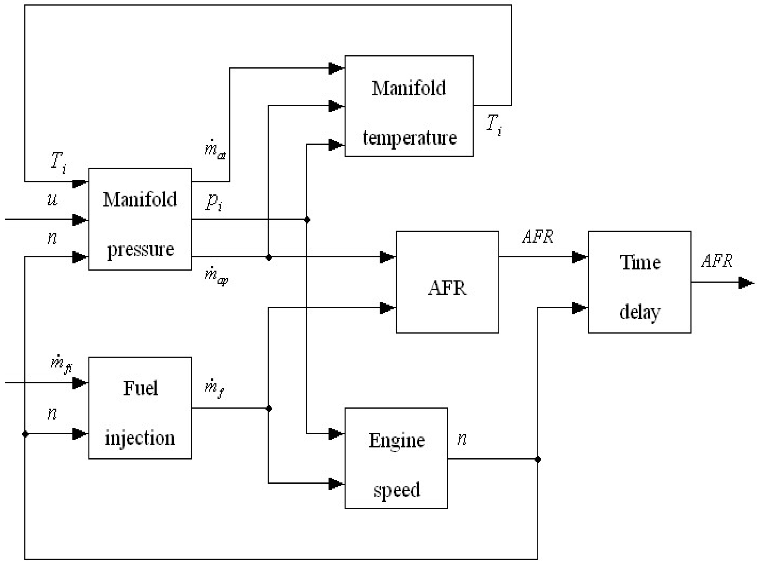
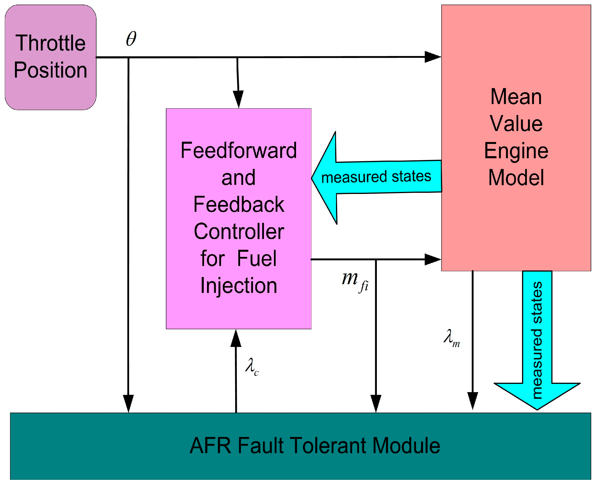
The time delay on the AFR measurement has not been considered in the original MVEM. A module used for AFR measurement is added into the original MVEM for the purpose of AFR control, which is based on Equation (16). The expanded system is shown in Figure 1, where it has two inputs —fuel injection rate $m_{fi}$ and throttle angle u; and one output—AFR.

Usually the throttle plate in the closed position is 9°–12°. Using this convention, the maximum opening angle of the throttle (if it is to be effective) is about 70°–80°. As described before, an electric pulse is triggered by the ECU to control the solenoid in the fuel injector. Therefore, the fuel injection rate can be controlled by adjusting the duty cycle in each sample time. For the expanded engine model in this paper, the fuel injection rate ranges from $6.28\times {10}^{-4}$ kg/s to $3\times {10}^{-3}$ kg/s.

3. Neural Network-Based Engine Modeling and Control

3.1. Radial Basis Function Networks

Radial basis function networks (RBFN) view the design of a neural network as a curve-fitting problem in a high-dimensional space. In contrast to the multi-layer perceptron network (MLPN), the RBFN utilizes a radial construction mechanism. This gives the hidden layer parameters of the RBFN a better interpretation than for the MLPN. In order to minimize the squared error between actual and estimated output, the algorithm adjusts the output layer weights, which is a linear learning rule [19]. The very well developed linear learning algorithms exhibit much faster convergence than nonlinear algorithms, such as least square (LS). In this research, the RBFN is adopted to model the dynamics of the AFR in SI engines.

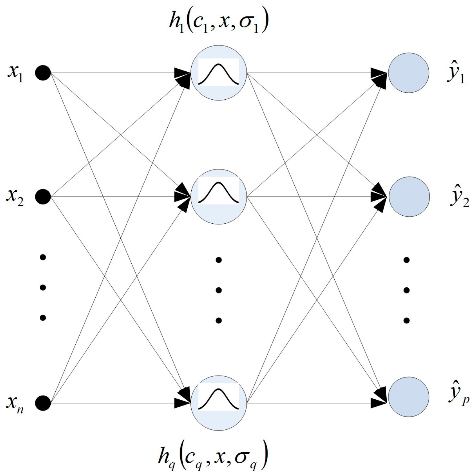
The RBFN, as shown in Figure 2, consists of three layers: an input layer, hidden layer, and output layer, where $x={\left[x_1,x_2,\cdots ,x_n\right]}^T\in R^n$ is the input vector, $h={\left[h_1,h_2,\cdots ,h_q\right]}^T\in R^q$ are the hidden layer nodes, $W\left(k\right)\in R^{p\times q}$ is the weight matrix with entry $w_{ij}$, which is the weight linking the jth node in the hidden layer to the ith node in the output layer, and $\widehat{y}=\left[{\widehat{y}}_1,{\widehat{y}}_2,\cdots ,{\widehat{y}}_p\right]\in R^p$ is the output vector of the RBFN.

In mathematical terms, we have the following equations to describe the RBFN:

$$\widehat{y}\left(k\right)=W h\left(k\right)$$

(17)

$$h\left(k\right)=f\left[z\left(k\right)\right]$$

(18)

$$z_i\left(k\right)=\sqrt{{\left[x\left(k\right)-c_i\right]}^T\left[x\left(k\right)-c_i\right]}=||x\left(k\right)-c_i||$$

(19)

where i = 1, 2, …, q. $c_i\in R^n$ is the ith centre in the input space, and $f[·]$ is the nonlinear activation function in hidden layer. The Gaussian basis function given by:

$$f\left[z\left(k\right),\mathsf{\sigma }\right]=e^{-\frac{z^2\left(k\right)}{{\mathsf{\sigma }}^2}}$$

(20)

where σ is a positive scalar called width, which is a distance scaling parameter to determine over what distance in the input space the unit will have a significant output.

The RBFN model is used in this paper to predict system outputs. The procedure of RBFN modelling and prediction is to determine the network inputs according to system dynamics, data collection and scaling, network training and validation, and using the network for prediction. The network training includes determining the number of nodes in the hidden layer, q, appropriate centres and widths, $c_i$ and ${\mathsf{\sigma }}_i$, $i=1,\dots ,q$ from the training data set, obtaining the weights W by training data, and validating the network by the test data. By considering the balance between the modeling performance and computational burden, the number of nodes in the hidden layer is determined by trial and error; centres and widths are found by a k means algorithm and $\mathsf{\rho }$ neighbourhood method, respectively; a recursive LS algorithm is adopted to update the weight W.

3.2. Engine Data Collection

In engine data collection, the training data must be representative of typical plant behavior in order to analyze the performance of different engine models in practical driving conditions. This means that input and output signals should adequately cover the region in which the system is going to be controlled [20]. 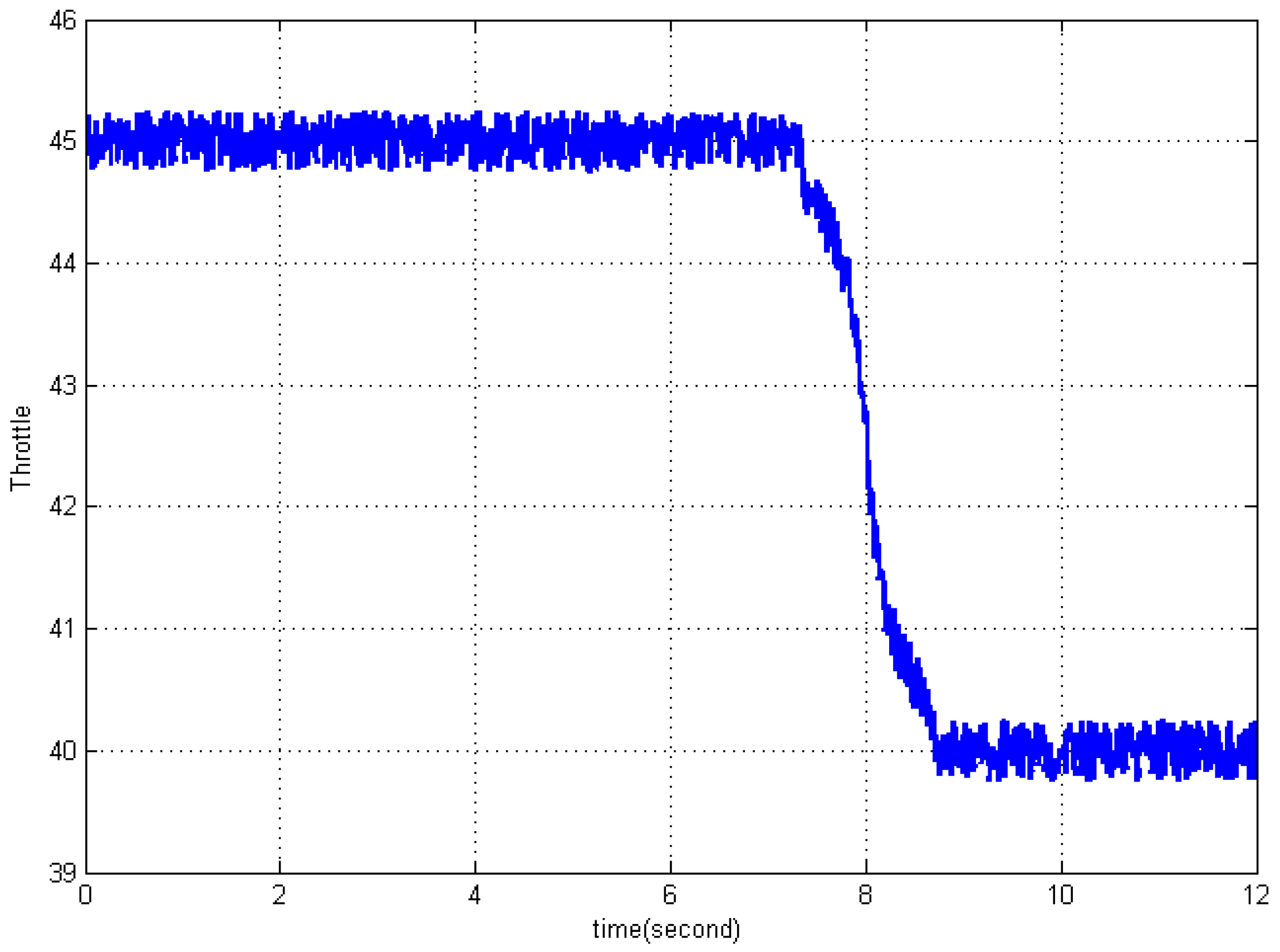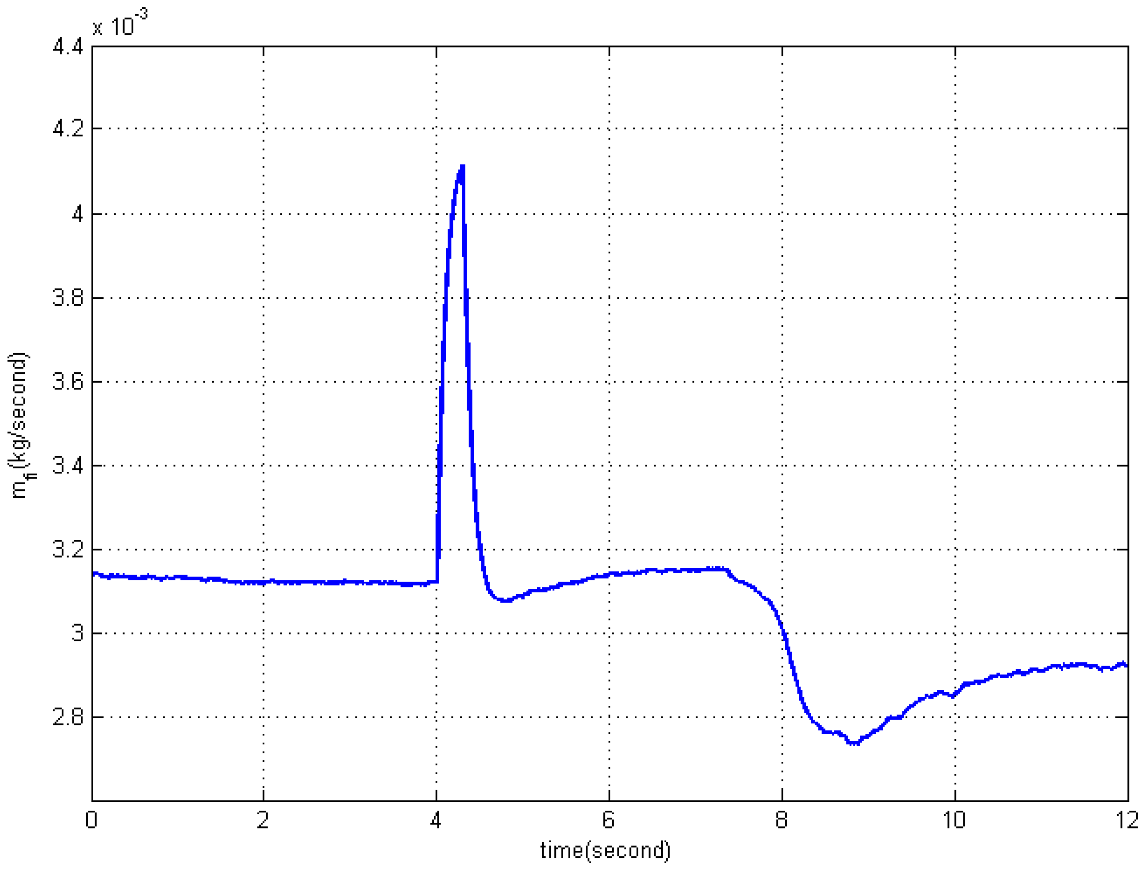As shown in Figure 1, the engine model has two inputs—fuel injection rate ${\dot{m}}_{fi}$ and throttle angle u; and one output—AFR. To obtain the engine data for neural network training, a set of random amplitude signals (RAS) was designed for throttle angle and fuel injection. As shown in

Table 1. Range of excitation signals for AFR modeling using RBFN. RAS: random amplitude signals.

RAS	Min	Max
u	20°	70°
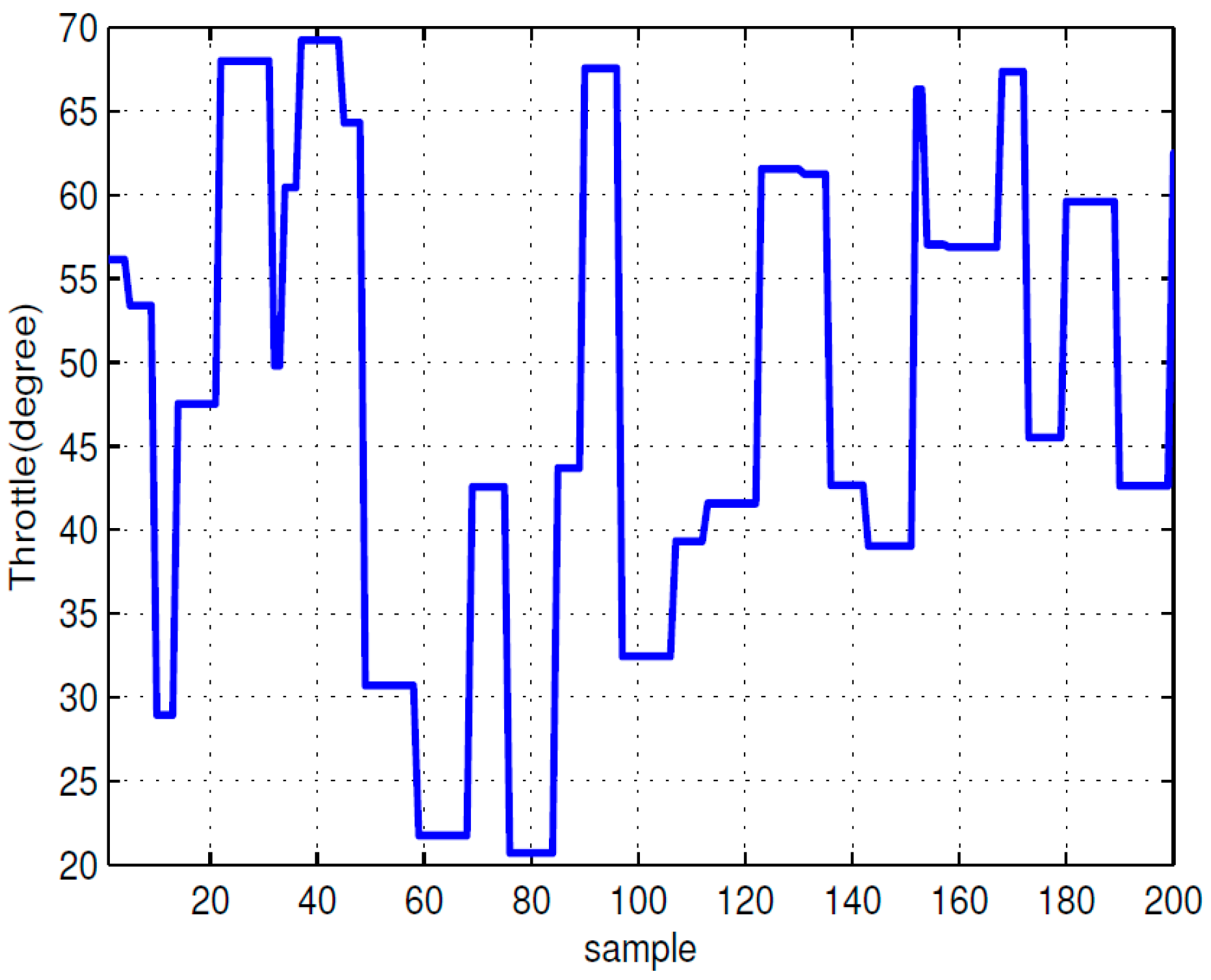
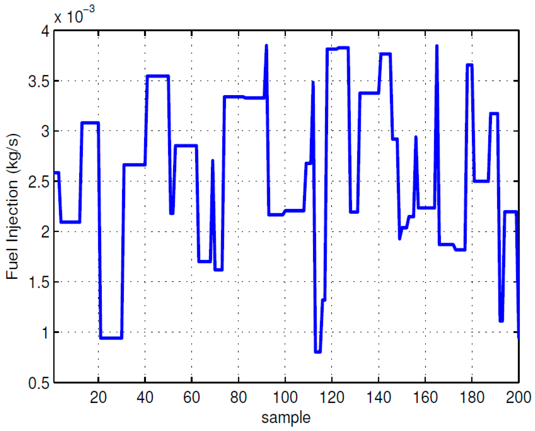
${\dot{m}}_{fi}$	7 × 10−4	3 × 10−3

, throttle angle was bounded between 20° and 70° and the fuel injection rate range used in the simulation engine is from 0.0007 to 0.0079 kg/s; the sample time is set to be 0.01 s.

The first 200 samples of excitation signals for engine model inputs are shown in Figure 3 and Figure 4. After introducing the excitation signals to the engine model in Figure 1, we can collect the data on the engine states, such as intake manifold pressure, intake manifold temperature, engine speed, and air fuel ratio, as the outputs. A set of 5000 data samples obtained was divided into two groups. The first 4500 data samples were used for training the RBFN model and the rest would remain for model validation.

Before the input and output of the engine data are used for training and validation, a linear scaling equation is used to process the data to make the range of engine data as [0, 1]:

$$x_s=\frac{x-x_{min}}{x_{max}-x_{min}}$$

(21)

In this research work, two RBFN models are trained to construct the feedforward controller. In addition, a soft sensor for the AFR is realized by the RBFN.

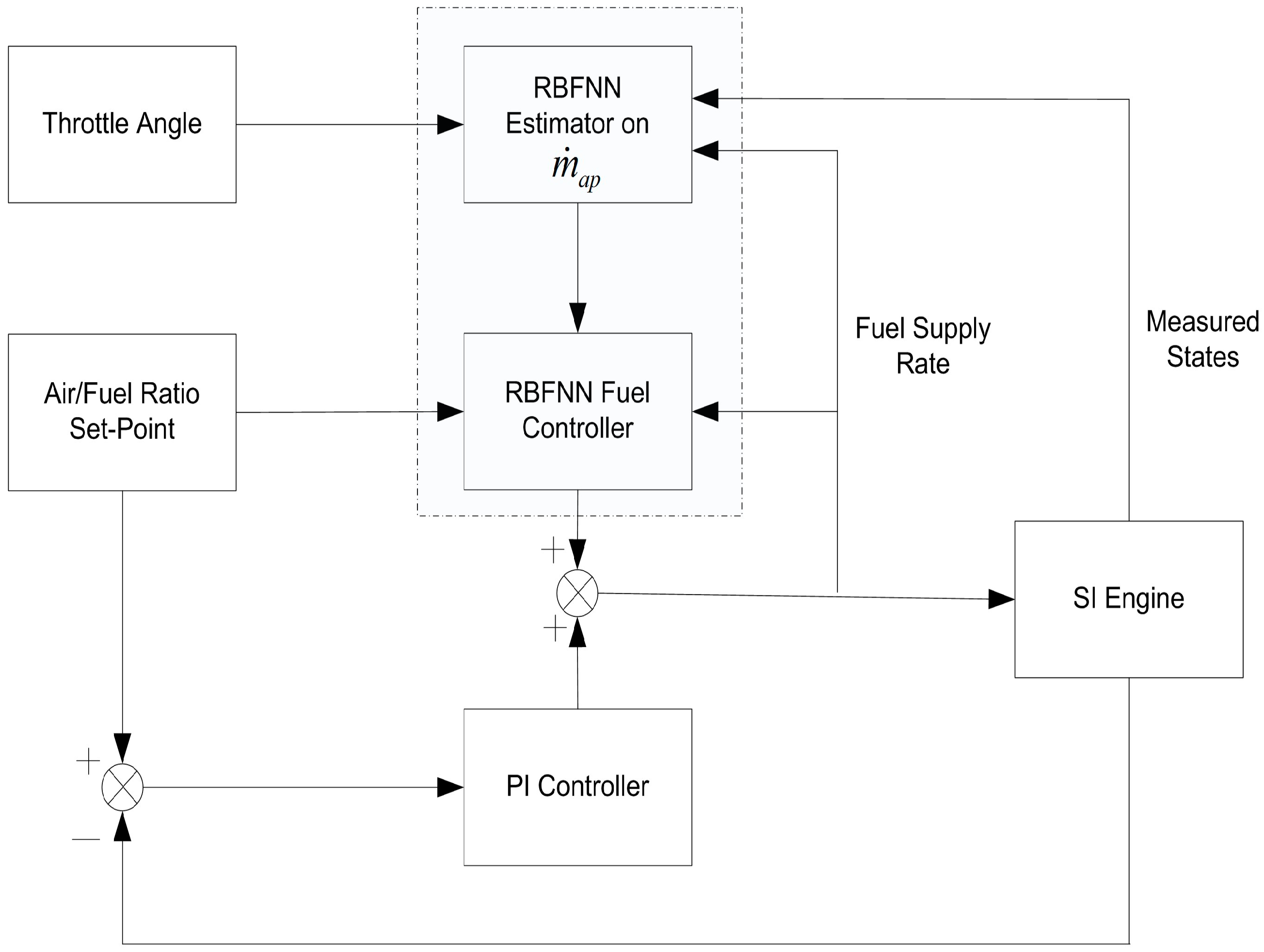
3.3. Neural Network-Based Feedforward and Feedback Scheme for Air/Fuel Ratio Regulation

A feedforward and feedback scheme for AFR regulation has been proposed by Zhai and Yu [21]. In this scheme, the feedforward controller consists of two RBFN models. One is for the intake manifold air dynamics and the other for fuel filming dynamics. The feedforward controller uses the measured states of the SI engine to predict the air flow rate into the engine port. The desired fuel inject rate is then calculated according to the output of the inverse model for fuel filming and the stoichiometric value of the SI engine combustion condition, which is 14.7 for ordinary gasoline engines. The advantage of the feedforward controller is that it can measure the system disturbance and make a corresponding action before the disturbance upsets the system. In this control scheme, the change of the throttle angle is identified as the disturbance that is generated by the vehicle driver, which cannot be controlled, but can be measured. The feedforward controller is essential to ensure the control performance during transient phase. However, to eliminate the steady state error in AFR regulation, the feedforword controller has to work together with a PI controller that is achieved by Ziegler and Nichols’ tuning method.

The structure is shown in Figure 5. The feedforward controller with two RBFN models is in the box with the dashed line. This structure is similar with the practical application in the automotive industry, which adopts look-up table as the feedforward controller. A more detailed advantage brought by the design can be found in Zhai and Yu’s paper [21]. In this research, the control scheme described above is expanded by including a fault-tolerant module.

3.4. Radial Basis Function Network-Based Soft Sensor for Air/Fuel Ratio

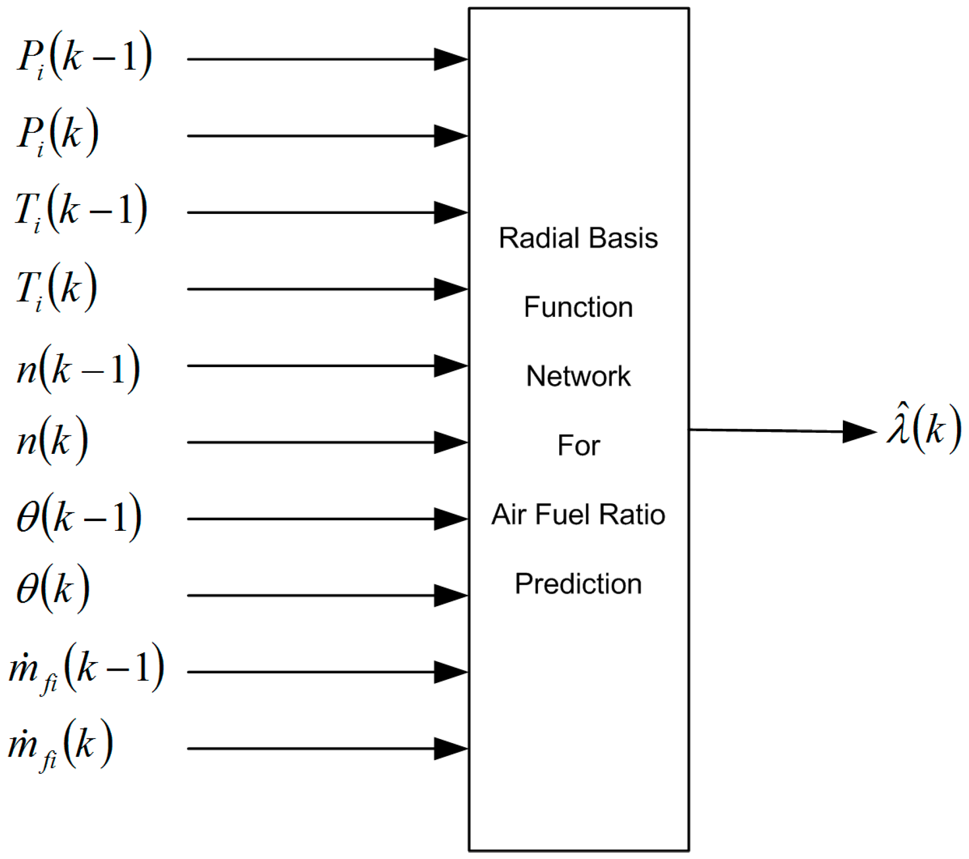
The wideband O₂ sensor, also called a wide-range air fuel (WRAF) sensor, is widely equipped in modern automotive vehicles to replace the traditional zirconia oxygen sensor that produces only a binary sequence for the AFR. Engine control management systems can control the air/fuel mixture at the stoichiometric ratio inside the combustion chamber using the measured signal by the WRAF. Since sensors are usually located in the exhaust stream, a certain time-delay on the AFR measurement cannot be avoided, which is shown in Equation (16).

Due to the harsh working condition and aging effect, the measured AFR can be biased by the control circuits of the WRAF sensor. It has been reported in many practical applications that the quality control measures can be obtained by using a soft sensor and the stringent requirements imposed on hardware-based sensors can be reduced significantly. Following this idea, a soft sensor for AFR is constructed by using the RBFN model in this research. After studying the SI engine dynamics that are described in Equations (1), (2) and (9)–(12), the dynamics of the AFR can be represented by the following equation:

$$\widehat{\mathsf{\lambda }}=g\left(P_i,T_i,n,\mathsf{\theta },{\dot{m}}_{fi}\right)$$

(22)

Here, $g$ is a nonlinear function of the RBFN, which is used to map the input and output data of SI engines. Therefore, the RBFN-based soft sensor for AFR can be realized using the measured variables, such as throttle angle $\mathsf{\theta }$, fuel injection rate ${\dot{m}}_{fi}$, intake manifold pressure $P_i$, intake manifold temperature $T_i$, and engine speed n. Then, the AFR in the combustion chamber can be inferred as $\widehat{\mathsf{\lambda }}$, accordingly. Considering the nonlinearity and time-delay in engine dynamics, a second-order structure of RBFN is chosen to construct the soft AFR sensor. As shown in Equation (23) and its structure shown in Figure 6:

$$\widehat{\lambda }\left(k\right)=g\left[P_i\left(k-1\right),P_i\left(k\right),T_i\left(k-1\right),T_i\left(k\right),n\left(k-1\right),n\left(k\right),\mathsf{\theta }\left(k-1\right),\mathsf{\theta }\left(k\right),{\dot{m}}_{fi}\left(k-1\right),{\dot{m}}_{fi}\left(k\right)\right]$$

(23)

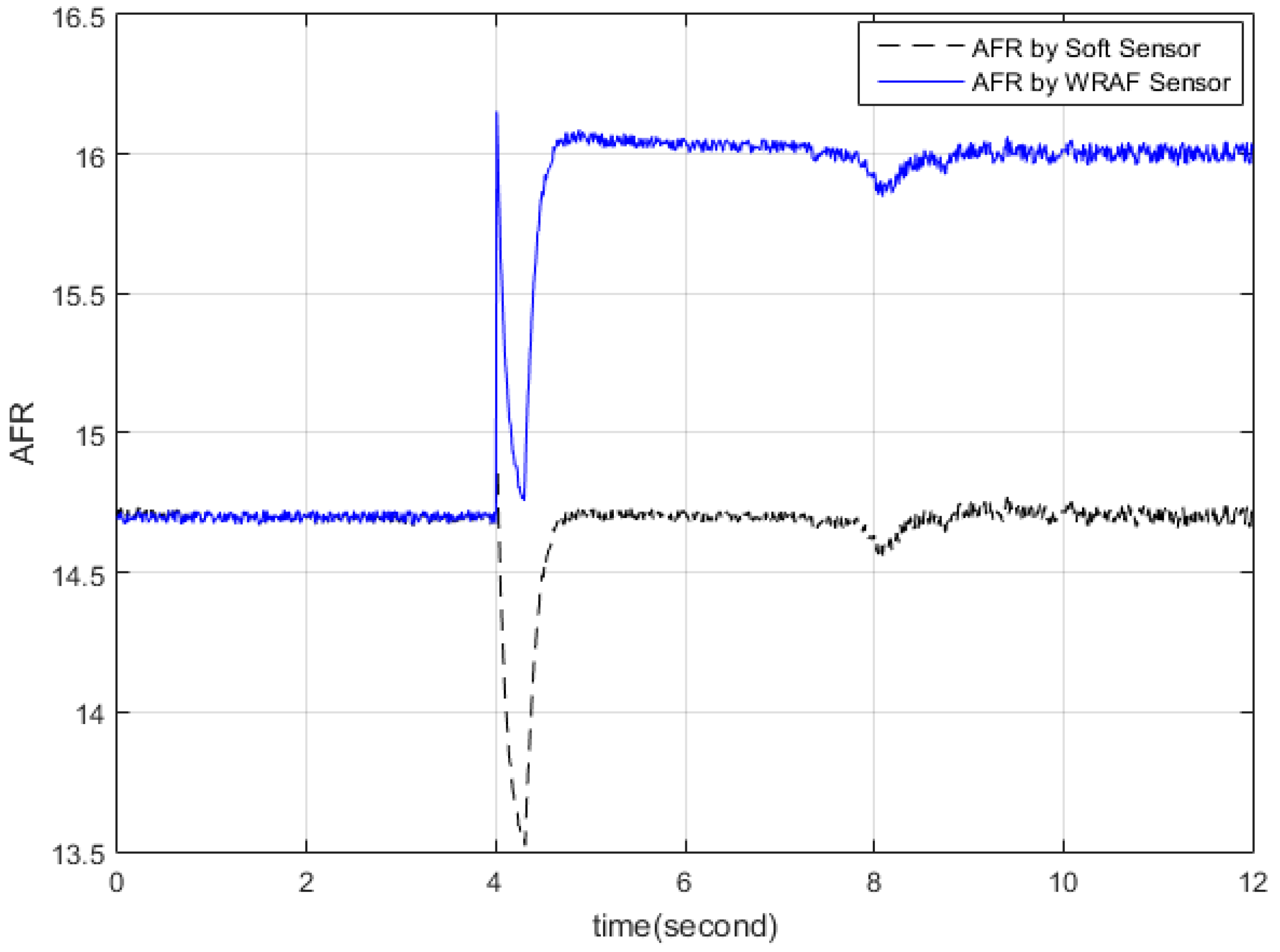
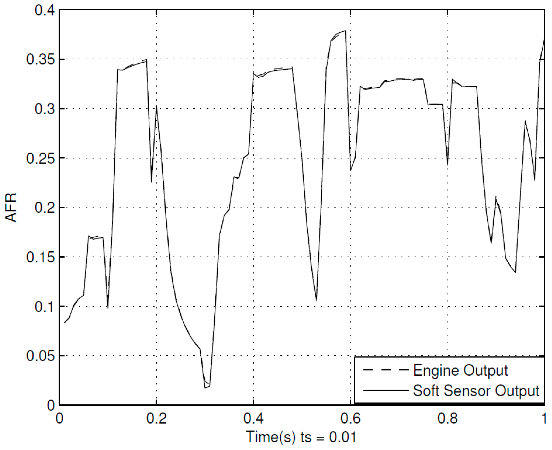
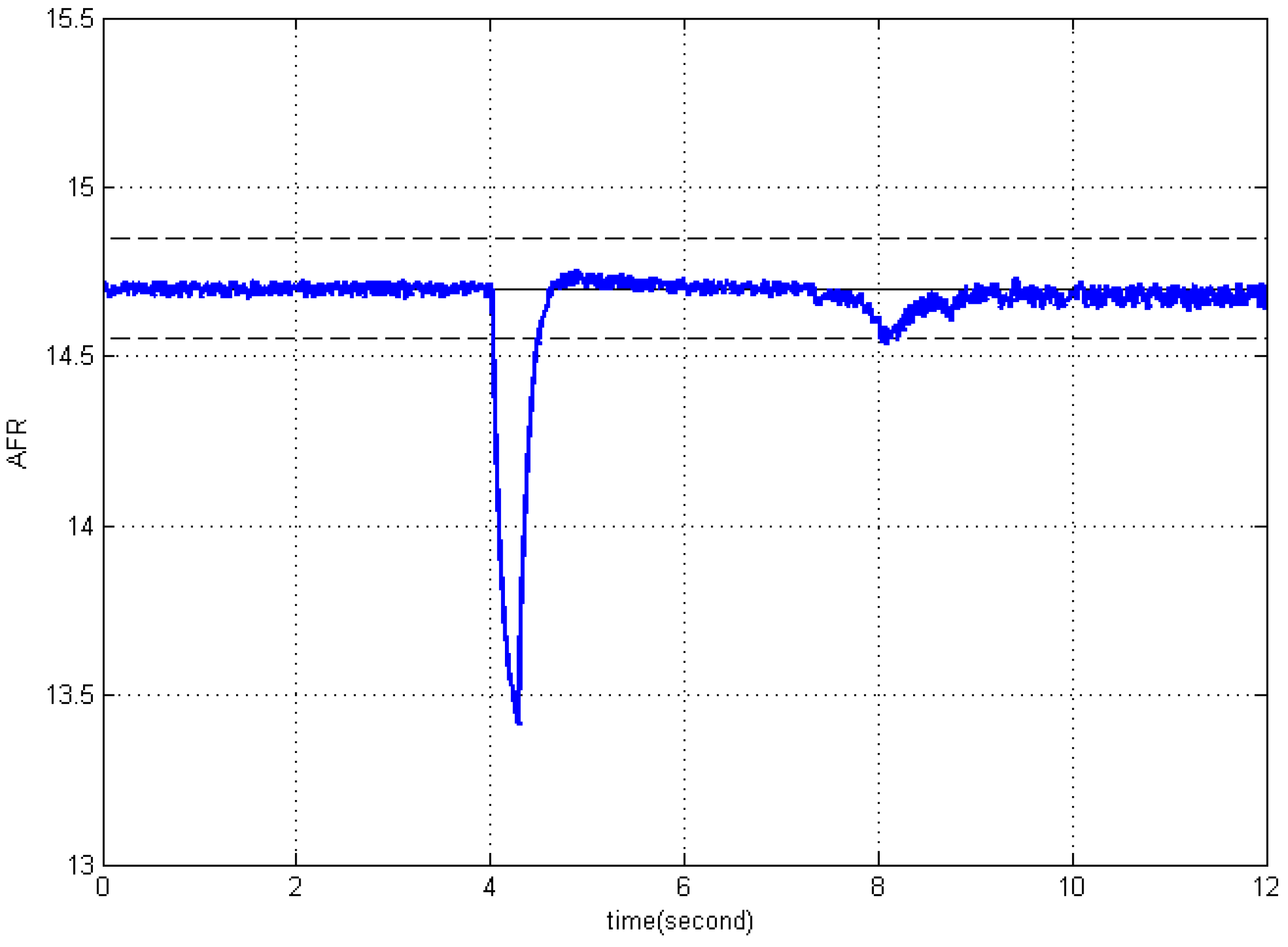
The soft sensor for AFR is used as a key component for the fault-tolerant module in this paper. The performance of the soft sensor is shown in Figure 7. The mean absolute error (MAE) of the shown 100 samples is 0.008. The details of its operation will be explained in Section 4.

4. Fault-Tolerant Control on Air/Fuel Ratio

4.1. Design of a Radial Basis Function Network-Based Fault-Tolerant Module

The main functions of an AFR fault-tolerant module are to monitor the measured signal quality of the AFR sensor and to provide appropriate compensation in the case of a sensor fault before it disturbs the desirable operating condition. This module consists of two parts. One is the AFR fault detection and the other the virtual switch of the AFR signal for feedback control. The operation rules for each part are described in the following sections.

4.1.1. Air/Fuel Ratio Fault Detection Using a Radial Basis Function Network-Based Soft Sensor

As shown in Figure 6, the engine input and engine states, such as throttle angle, fuel injection rate, intake manifold pressure, intake manifold temperature, and engine speed, are measured and used as the input for the RBFN-based soft sensor for AFR. Given a sampling interval k, the soft sensor can produce the predicted AFR value ${\mathsf{\lambda }}_p\left(k\right)$. A relative error ${\mathsf{ϵ}}_{\mathsf{\lambda }}\left(k\right)$ between ${\mathsf{\lambda }}_p\left(k\right)$ from the AFR soft sensor and the measured AFR ${\mathsf{\lambda }}_m\left(k\right)$ by the WRAF sensor can be obtained by the following equation:

$${\mathsf{ϵ}}_{\mathsf{\lambda }}\left(k\right)=\left|\frac{{\mathsf{\lambda }}_p\left(k\right)-{\mathsf{\lambda }}_m\left(k\right)}{{\mathsf{\lambda }}_p\left(k\right)}\right|$$

(24)

Theoretically, in the case that λ reaches its threshold, the experimental point is considered as a WRAF sensor fault. However, considering the practical application, the prediction error, sensor noise, or experimental uncertainties must be considered to avoid false alarms. In this research, the sampling interval for AFR measurement and fuel injection control are all assigned as 0.01 s, which is consistent with the engine control laboratory setting [22]. A sliding window of 0.3 s is adopted, which corresponds to 30 successive sampling intervals for control:

$${\mathsf{ϵ}}_{\mathrm{total}}={\displaystyle \sum }_{i=1}^{30}{\mathsf{ϵ}}_{\mathsf{\lambda }}\left(i\right)$$

(25)

If the MAE of this window exceeds the threshold $r_t$ determined by the designer by trial and error, the engine condition is identified as an AFR sensor fault. The fault-tolerant module at that moment can make a corresponding compensation on the AFR value for control. $r_t$ for ${\mathsf{ϵ}}_{\mathrm{total}}$ in this simulation is 1.5.

4.1.2. Virtual Switch of Air/Fuel Ratio Signal for Feedback Control

Under normal operating conditions, the fault-tolerant module provides the measured AFR value ${\mathsf{\lambda }}_m$ as the AFR for feedback controller ${\mathsf{\lambda }}_c$. However, if the fault detection part detects the WRAF sensor fault, the virtual switch will switch the AFR signal from ${\mathsf{\lambda }}_m$ to ${\mathsf{\lambda }}_p$. The operation of the virtual switch is shown in Equation (26):

$${\mathsf{\lambda }}_c=\{\begin{array}{c}{\mathsf{\lambda }}_m{\mathsf{ϵ}}_{total}\le r_t\\ {\mathsf{\lambda }}_p{\mathsf{ϵ}}_{total}>r_t\end{array}$$

(26)

As shown in Figure 7, the soft sensor for the AFR can achieve a high level of accuracy on AFR prediction. It can be seen that the controller using this compensated AFR value can still demonstrate satisfactory performance in terms of setpoint tracking, which is essential to reduce the pollution caused by engine emissions when a WRAF sensor fault happens. A signal flowchart of the time sequence is given in Figure 8, which demonstrates the operation of the fault-tolerant module.

4.2. Radial Basis Function Network-Based Fault-Tolerant Control Strategy

The diagram shows the complete structure of the fault-tolerant control strategy for AFR regulation in Figure 9. The direct connections between the feed-forward and feedback controller and the AFR fault-tolerant module are the manipulated variable ${\dot{m}}_{fi}$ and the AFR value ${\mathsf{\lambda }}_c$, which shows that the contribution of the fault-tolerant module to provides a reliable AFR value for the fuel injection controller. It has been proved in Section 4.3 by simulations.

4.3. Simulations and Results

The angle of the closed position of the throttle is between 9° and 10°. In this simulation, the throttle angle is set at 45° with 0.5% uncertainty to simulate the driving dynamics of the simulated engine. The set-point of AFR is set to the constant stoichiometric value 14.7. The AFR needs to be controlled between the 1% bounds of the stoichiometric value. The sampling time is 0.01 s for both measurement and control. After running the simulation for 4 s, a 10% over-reading on the AFR sensor is introduced to the control system. After 6.5 s, a smooth change of engine operating condition is applied by shifting the throttle from 45° to 40°, which is shown in Figure 10.

As shown in Figure 11, the AFR sensor fault that is introduced after 4 s resulted in a large overshoot in engine speed. This is because the controller’s fuel injection rate ${\dot{m}}_{fi}$ is misled by the biased signal given by the WRAF sensor with the fault. However, in the developed fault-tolerant module, this sensor fault has been quickly detected and the corresponding compensation is generated for the fuel injection rate. It can also be seen that, when the engine operating condition changes, proper control on the fuel injection rate can be produced by the controller to achieve satisfactory AFR regulation.

It can be seen in Figure 12 that, for both AFR sensor fault and changes in operating conditions, the AFR has been pulled back to the bounds of the stoichiometric value within seconds. The MAE for AFR tracking is 0.043.

Figure 13 shows the output for both the WRAF sensor and the developed soft sensor. When the WRAF sensor fault generates false information on the AFR, the developed soft sensor can still produce the acceptable AFR values for feedback control using the information on engine states and system inputs.

5. Conclusions

In this paper, a soft sensor for the AFR is developed using RBFN after the analysis of SI engine dynamics. The AFR soft sensor can predict the AFR with high accuracy. Based on the developed soft sensor, a fault-tolerant module to deal with the WRAF sensor fault is realized. It can also provide an appropriate AFR value for feedback control by switching between the predicted AFR by the soft sensor and the measured AFR by WRAF sensor.

Simulation results show that the sensor fault can be quickly detected by the fault-tolerant module given the specific window time. The whole control scheme can prevent the AFR from deviating from the acceptable bounds of the stoichiometric value.

In this research, the engine operating condition is changed after introducing a sensor fault into the SI engine system, to test the robustness of the proposed control scheme. The results show that satisfactory AFR tracking performance can be maintained for different operating conditions.