
Risk Assessment Method of UHV AC/DC Power System under Serious Disasters

State Key Laboratory of New Energy Power System, North China Electric Power University, Beijing 102206, China
*
Author to whom correspondence should be addressed.
Energies 2017, 10(1), 13; https://doi.org/10.3390/en10010013
Submission received: 10 November 2016
/
Revised: 14 December 2016
/
Accepted: 17 December 2016
/
Published: 23 December 2016
(This article belongs to the Special Issue Advances in Power System Operations and Planning)
Abstract
:Based on the theory of risk assessment, the risk assessment method for an ultra-high voltage (UHV) AC/DC hybrid power system under severe disaster is studied. Firstly, considering the whole process of cascading failure, a fast failure probability calculation method is proposed, and the whole process risk assessment model is established considering the loss of both fault stage and recovery stage based on Monte Carlo method and BPA software. Secondly, the comprehensive evaluation index system is proposed from the aspects of power system structure, fault state and economic loss, and the quantitative assessment of system risk is carried out by an entropy weight model. Finally, the risk assessment of two UHV planning schemes are carried out and compared, which proves the effectiveness of the research work.
1. Introduction
The construction and operation of the ultra-high voltage (UHV) power grid has played a huge role in promoting social development. However, its safety has been widely concerned by the community [1,2]. Scientific evaluation of the safety of the UHV grid is of great significance to analyze the security level of the power system, find the potential safety problems and prevent the blackouts. “N-1” or “N-2” guidelines are the conventional methods for assessing grid security [3,4], and some scholars have proposed improved methods or indicators for UHV grids [5,6,7]. However, these methods have two disadvantages: on the one hand, it only analyzes the consequences of failure events of single (double) elements, ignoring the probability of its occurrence. In fact, systemic risk is the combination of probability and consequence; on the other hand, it can not reflect the disaster-resistant performance under serious disasters with multi-component failure. In fact, the cascade fault characteristic is an important aspect that reflects the safety level of the power system [8].
According to the nature of fault triggering, the cascading faults can be divided into three types: overload dominant, protection dominant and structure dominant [9]. In [10,11], the transfer of post-fault flow is taken as the selection principle of N-K fault, and the influence of wind farms on power system risk is analyzed, but the model is lack of discussion on the protection hidden fault. In fact, the hidden faults cause great harm to the safety of the system. In [12,13], a protection hidden fault model is established, and the protection misoperation probability is calculated and applied to the simulation of cascading failures. However, the model lacks a discussion on the system loss during the fault recovery phase. The above studies have been focused on the overload dominant, protection dominant, but the studies on structure dominant faults caused by natural disasters are few. In [14], a cloud model and fuzzy comprehensive evaluation (FCE) method is proposed for collecting and monitoring the space charge density in an ultra-high-voltage direct-current (UHVDC) environment. In [15], the risk assessment model of an earthquake disaster on the power system is established, and the influence of the network structure and operation conditions on the seismic performance of the power system is studied. The risk index in [14,15] is single, which contains system state or loss index, but lack of a set of evaluation index systems for a UHV AC/DC power grid.
The development process of system cascading failure under severe disaster is shown in Figure 1. In severe disaster, the system structure is destroyed, and then cause line overload and protection malfunction, often contain three dominant types, which need comprehensive analysis; the process of cascading failure has not been adequately simulated in above references, in fact, the system still has risk loss in the process of fault recover; at the same time, the risk index is not comprehensive enough, and it needs to analyze the system structure, fault state and failure loss comprehensively. Finally, the simulation examples are based on the simulation system, which can not truly reflect the nature of the real AC/DC power system.
Based on the above research foundation and analysis, this paper presents a whole process risk analysis model under severe disaster. Based on the BPA stabilization procedure, this paper analyzes the cascading faults of UHV AC/DC power grid, and provides reference for the evaluation of system risk level.
2. Chain Failure Model
2.1. Chain Failure Probability Calculation
In the traditional method, a sequential Monte Carlo method and Bayesian model are usually adopted to develop the fault and calculate probability of failure. Under the large network, the computation and time-consuming are huge. In order to improve the computational efficiency, this paper combines the non-sequential Monte-Carlo method and BPA to calculate the probability of chain failure. First, make the following assumptions:
- (1)
- Outage of the components can usually be divided into two types: independent outages and related outages. Due to the short duration of severe disasters (such as earthquakes and typhoons), the independent outages consider the forcible outage models in which the failure can be repaired. The related outages consider the environmental interdependence and interlocking models, and do not consider the plan outage and aging failure.
- (2)
- The failure rate of the component is constant during the fault and no new fault occurs during system recovery.
- (3)
- All initial faulty components fail simultaneously under the hazard (taking into account the most severe three-phase permanent short-circuit) and are independent of each other. The subsequent failure caused by the initial failure must occur under the conditions of the simulation, which can be considered a conditional probability of 1, so we only need to calculate the probability of occurrence of the initial set of failures.
- (4)
- Since the probability of protection fault is low, only the primary protection faults developed by the initial failures set are taken into account.
The calculation steps are as follows:
- (1)
- First of all, the disaster history database is established to predict the area where the disaster may occur in the future. Combining with the data of component damage under the disaster of a domestic power system, the fault probability value of electrical equipment is calculated and the data is provided for the risk assessment.
- (2)
- According to the prediction result of disaster area, the initial fault set (including the protection hidden fault) is set up, and the simulation is carried out in BPA to get the chain fault.
- (3)
- The system state is sampled by non-sequential Monte Carlo method, and the component failure frequency and average repair time are calculated. The relevant calculation is as follows [16]:where fto is the average failure frequency; rto is the average repair time; fad and fno are the failure frequencies under severe and normal climatic conditions, respectively; rad and rno are the mean repair times under the severe and normal climatic conditions, respectively; and Pad and (1 − Pad) are probabilities of severe and normal climatic conditions, respectively.Since data acquisition systems usually do not distinguish between failure events in normal and severe climates, only the average failure frequency and mean repair time in the past years are available. Therefore, two parameters, F and M, can be introduced, where F is the percentage of failures that occur under adverse climates and should be between 0 and 1. M is a multiple of the repair time under severe weather conditions compared to normal climatic conditions and must be equal to or greater than 1. Normally F and M can be estimated from engineering judgment. From the definitions of F and M, the variables relationship shown in Equation (3) can be derived from Equations (1) and (2):
- (4)
- After the average failure frequency and average repair time are obtained in step 3, the component failure rate can be calculated and the probability of the initial fault set can be calculated. Under simulation conditions, that is, chain failure rate, as shown in Equations (4)–(6):where is repair rate, is failure rate, t is the faulty component, E is the initial failure rate of the system, and 8760 is the number of hours of one year.
2.2. The Control Strategy after Fault and the Termination Condition of Fault
A reasonable voltage and frequency control scheme is very important to ensure the safe operation of the system with UHV transmission lines. In this paper, according to “Power System Safety and Stability Guidelines”, we configure three lines of defense in the BPA for critical failures: (1) the first line of defense: protection; (2) the second line of defense: security and stability control system, including automatic reclosing, automatic bus transfer equipment, chain cutting machine, load shedding, etc.; and (3) the third line of defense: deserialization, low-frequency and low-voltage load shedding.
Based on BPA simulation, we set the following fault stopping conditions: (1) after a certain calculation, there is no new fault, that is, no new component overload and no voltage violations, and the system reaches a new equilibrium; (2) the power flow is not convergent after a fault, or the power flow also can not converge after adding the control measures, , then the grid is considered to collapse.
2.3. Fault Recovery Method
After the chain failure, fault components will be thoroughly repaired, so that there is no new hidden fault before repair, and then the power supply to the loss of load will be gradually restored. Restoration needs to first emulate the maximum power flow that the line allows to ascend:
where is the maximum power that the kth branch can pass; is the branch recovery factor, and the value depends on the degree of damage to the line.
We take the minimum load power loss and switching operations as the goal and gradually restore power supply. In the recovery process, we need to simulate the line voltage in order to prevent the occurrence of new failures. When the bus voltage rises to V1, the load is restored to a%. When the bus voltage rises to V2, the load is restored to b%. When the bus voltage rises to V3 (V3 > V2 > V1), the load is restored to c%. The risk assessment process is complete until all loads are restored.
2.4. Calculation of System Risk Indicators
On the basis of the risk assessment of the whole process, the system's loss load is calculated and the risk index of the system is completed.
3. System Risk Indicators
The UHV power grid has the following advantages: large transmission capacity, wide coverage, saving the transmission line corridor, and a decrease in the ratio of active power loss. However, it also has certain unhealthy characteristics, mainly embodied in:
- (1)
- In the UHV power grid, with more load placement, the transmission distance is far. Therefore, the grid structure has a great influence on the grid operation and stability.
- (2)
- In the AC/DC hybrid transmission structure, the sending and receiving ends still keep running synchronously. The stability problem of the transmission line is mainly caused by the short circuit fault of the AC system and the commutation failure of the DC system, and the large-scale power flow caused by the latch-up fault, resulting in long-distance transmission channel station voltage stability problems and transient power angle stability problems.
Therefore, the chain failure risk assessment index should not only reflect the seriousness of the accident, but also highlight the weakness of the grid structure. At the same time, special indicators should be included to meet the characteristics of UHV AC/DC power grids. Therefore, this paper establishes the risk assessment index system from the power system structure, fault state, and economic losses, as shown in Table 1.
3.1. Power System Structure Index
The structure of the grid has important influence on the stability of the system, so the static risk assessment of the grid structure is needed. The basic parameters describing the statistical properties of the complex network topology are called the structural feature quantities. The most important parameters include average length of line (ALL), node medians and node degrees [17], while multi-infeed short-circuit ratio (MISCR) [5] is used as the indicator of the strength of the multi-infeed AC/DC system.
(1) Average length of line (ALL)
Define ALL as the average of the shortest path length between any two nodes, that is
where is defined as the length of the shortest path connecting node i and node j; N is the number of nodes in the network, and K is the number of network edges. Generally, the higher the ALL value is, the lower the system reliability is.
(2) Network average medians (NAM) and Network average degrees (NAD)
The degree of node i is the number of edges connected to the node. The median of node i refers to the number of the shortest path through the node in the network. Degrees and medians can reflect the importance of nodes in the network, that is, the larger value of the nodes in the network are more important. The expected value of the degrees and medians are network average degrees (NAD) and network average medians (NAM), respectively. The higher the value is, the stronger the system coupling is.
(3) Multi-infeed short-circuit ratio (MISCR)
Because of the close electrical connection between the DC converter stations of the multi-DC infeed system, if the simple short-circuit ratio is used to evaluate the multi-DC infeed system, there will be a large deviation, and the results are obviously optimistic. Therefore, for a multi-DC infeed system, MISCR can better evaluate the strength of an AC/DC link system, and a strong short-ratio system is more reliable. The MISCR is defined as:
where MISCRm is the MISCR value for the mth DC line; Zeqmm is the self-impedance of the mth DC line in an equivalent impedance matrix; Zeqmn is the mutual impedance between the mth DC line and the nth DC line in an equivalent impedance matrix; Pdm is the rated power of the mth DC line; Pdn is the rated power of the nth DC line; and M is the total number of DC lines.
Take the expected value of MISCRm as the system MISCR value.
3.2. Fault State Index
Voltage risk and frequency risk are two basic risk indicators that reflect the state of the power system. At the same time, the synchronous operation is an important characteristic of the stability of the system in the AC/DC mixed gird with more DC lines. Therefore, the power angle difference between units is taken as one of the risk indicators.
(1) Low voltage severity (LVS)
The two low voltage severity (LVS) functions in Figure 2 show the effect on the system when the bus voltage amplitude decreases. The discrete function is defined as: the value of the function is 1 when the bus voltage falls below the defined voltage threshold of 0.95 p.u.; otherwise, the value is 0. The continuous function is defined as: when the voltage value of the bus is 0.95 p.u., the function value is 1. When the voltage level drops further, its function value increases linearly. It overcomes the shortcoming of the discrete function. The value of the function can reflect the voltage level.
In this paper, the continuous function is used, as shown in Equation (10):
where is the voltage value of the kth bus and , is the severity.
In the BPA stabilization procedure, the simulation results will give the bus voltage with the lower bus voltage. The system LVS is defined as:
where and are the LVS weights (this paper takes equal weight), is the mean LVS, and is the maximum LVS.
(2) Power angle difference severity (PADS)
Similar to the LVS function, the power angle difference severity (PADS) function of the units also includes two forms of functions, as shown in Figure 3. In this paper, the continuous function is used, as shown in Equation (12):
where is the pth power angel difference, and is the severity.
The system PADS is defined as:
where and are the PADS weights (this paper takes equal weight), is the mean PADS, and is the maximum PADS.
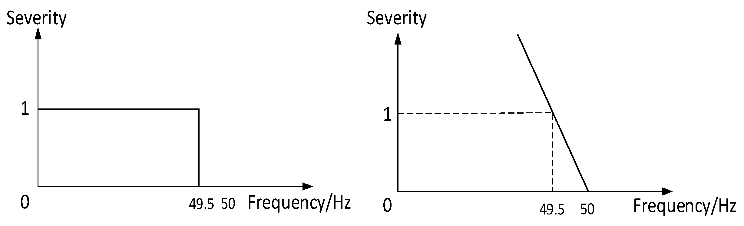
(3) System frequency severity (SFS)
In the system frequency severity (SFS) function, the risk is 0 for system frequency of 50 Hz and 1 for a deviation of 0.5 Hz, as shown in Figure 4. In this paper, a continuous function is adopted, as shown in Equation (14):
where f is the system frequency and , is SFS.
3.3. Economic Losses Index
The load of each bus can be divided into two parts, including which can be power cuts or not. For each fault condition (including fault phase and recovery phase), which may lead to load shedding or forced load reduction, calculate its power loss (PL), and then accumulate the PL value in each stage, resulting in the whole process PL function:
where is the total PL cost (Yuan); and are the load reduction variables (MW·h) for users, which can be power cuts or not in the kth bus during the nd accident phase; and are the unit cost of power outages (Yuan/MW·h) for users, which can be power cuts or not; is the weighting factor reflecting the importance of bus load, since the BPA procedure does not distinguish the severity of the load. Therefore, we take = 1.
3.4. Comprehensive Risk Assessment
Entropy is a method of calculating the information difference between random vectors. It can determine the degree of support by judging the degree of intersection between different information sources (this paper refers to all kinds of risk indicators) and determining the weight of the information source according to the support degree. The higher the degree of support, the greater the weight. It overcomes the subjective arbitrariness of index weights. In this paper, the entropy method [18] is used for comprehensive risk assessment.
Because of the inconsistency between the dimensions of the indicators, they need to be standardized and normalized, as follows:
where is the standardized matrix of indicators, is the qth indicator, and are its maximum value and minimum value, is normalized index matrix, and Q is the total number of indicators.
For the indicators for which the smaller the value, the greater the risk, such as MISCR, NAM and NAD, first take its reciprocal, and then use Equations (16) and (17) to calculate.
According to the concept of entropy, the entropy of each index is defined as
The entropy weight of the qth index is
The final risk value of each index is the product of its entropy weight, index value and system failure probability, as follows:
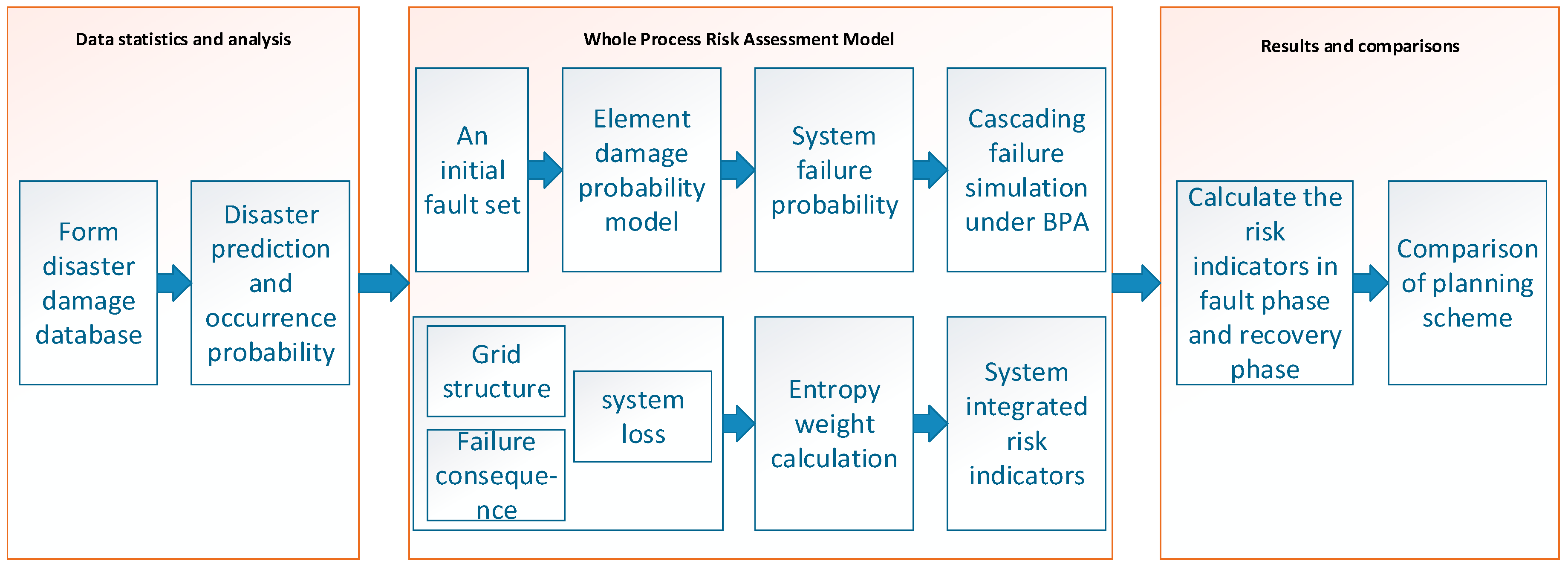
The calculation flow of this paper is shown in Figure 5:
4. Case Study
4.1. Case Introduction
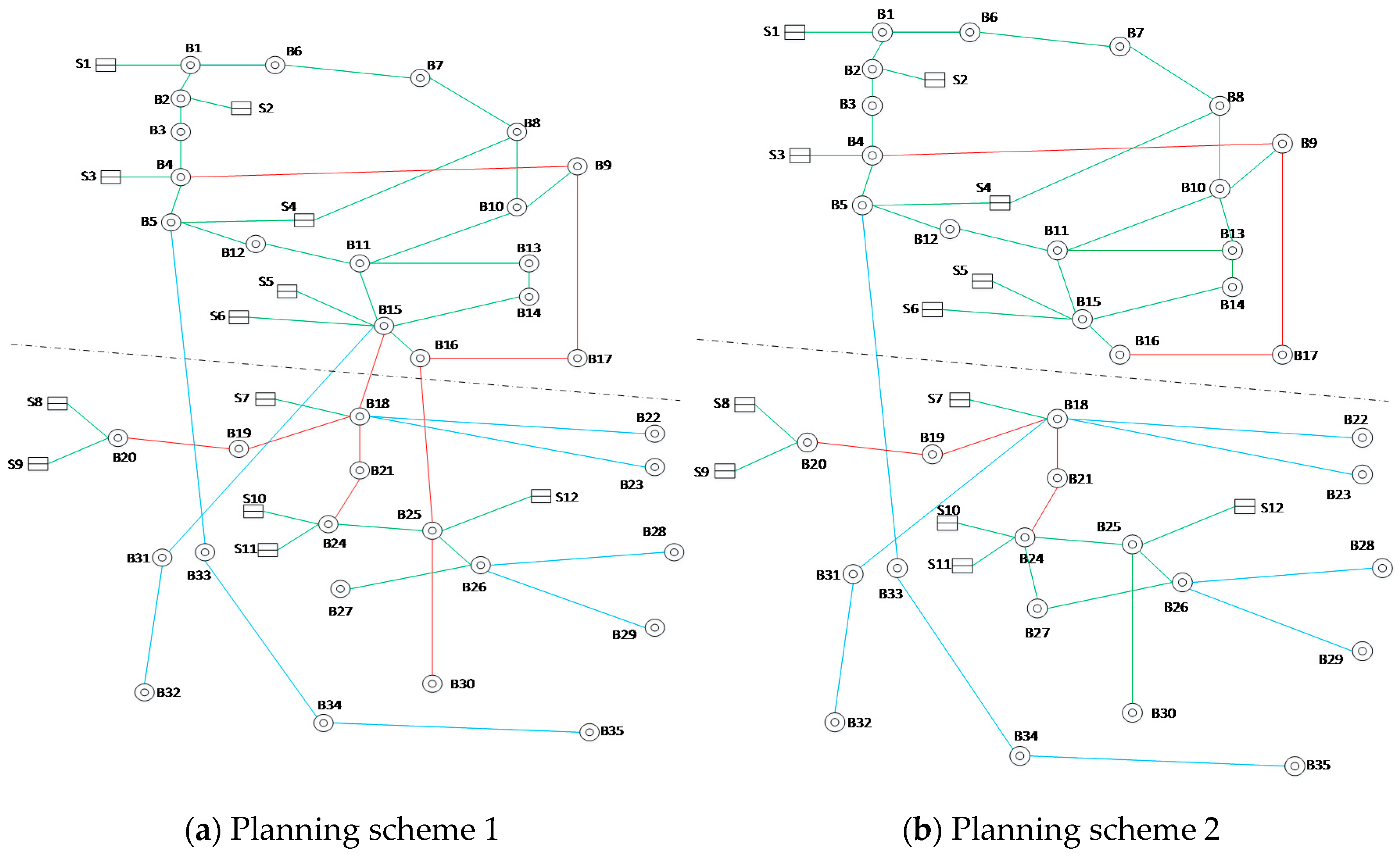
In order to verify the correctness of the proposed model in this paper, we adopt a regional power grid. The area takes 500 kV lines as the main grid structure, with the total installed capacity of 10.2589 million kilowatts and transmission load of 7.47 million kilowatts (winter big way). North and south regions form two independent power grids, and there are security and stability issues including a power surplus and a weak grid structure. In order to improve the grid structure, two kinds of target UHV grid planning schemes are proposed, as shown in Figure 6. The green line represents AC 500 kV, red represents AC 1000 kV, blue represents DC ± 800 kV, S represents source, and B represents the node (converter station, substation and load). The simulation is performed on PSD-BPA version 2.0 (China Electric Power Research Institute, Beijing, China) (Copyright by China EPRI, 2010).
Planning scheme 1 (P1): based on the 1000 kV UHV AC power grid (B4–B30, B15–B24, B18–B20), to achieve the north–south regional system connecting and the total regional synchronous operation, with the construction of ±800 kV DC (B5–B35, B18–B22, B18–B23, B26–B28, B26–B29, B15–B32) external transmission, to solve the problem of power surplus.
Planning scheme 2 (P2): The construction of regional 1000 kV UHV (B4–B16, B18–B24, B18–B20) and 500 kV (B10–B13, B25–B30, B24–B27) lines to strengthen the regional grid structure, considering the possible spread of accidents in the disaster state, the north and south still keep running asynchronously. A DC high voltage scheme will convert B15–B32 to B18–B32.
The investment of the two schemes is basically the same and meets the requirements of “N-1” and “N-2”, and the risk evaluation model proposed in this paper is used to compare and analyze the two schemes.
4.2. The Initial Failure Set and the Results of Chain Failure
From the analysis of the historical disaster database of the area, it is easy to be affected by earthquake disasters south of the dividing line. In this paper, we consider the common mainshock–aftershock type earthquakes with short duration (usually lasting several tens of minutes), but the main shock is very harmful. The initial failure set is studied in two cases.
Case 1: Do not consider the protection hidden fault. The initial failure set is: S7, S10, S11, S7–B18, S10–B24, S11–B24, B18–B19, B18–B21, and B21–B24.
Case 2: Consider protection hidden faults. Based on Case 1, B19 and B24 export main protection malfunctions.
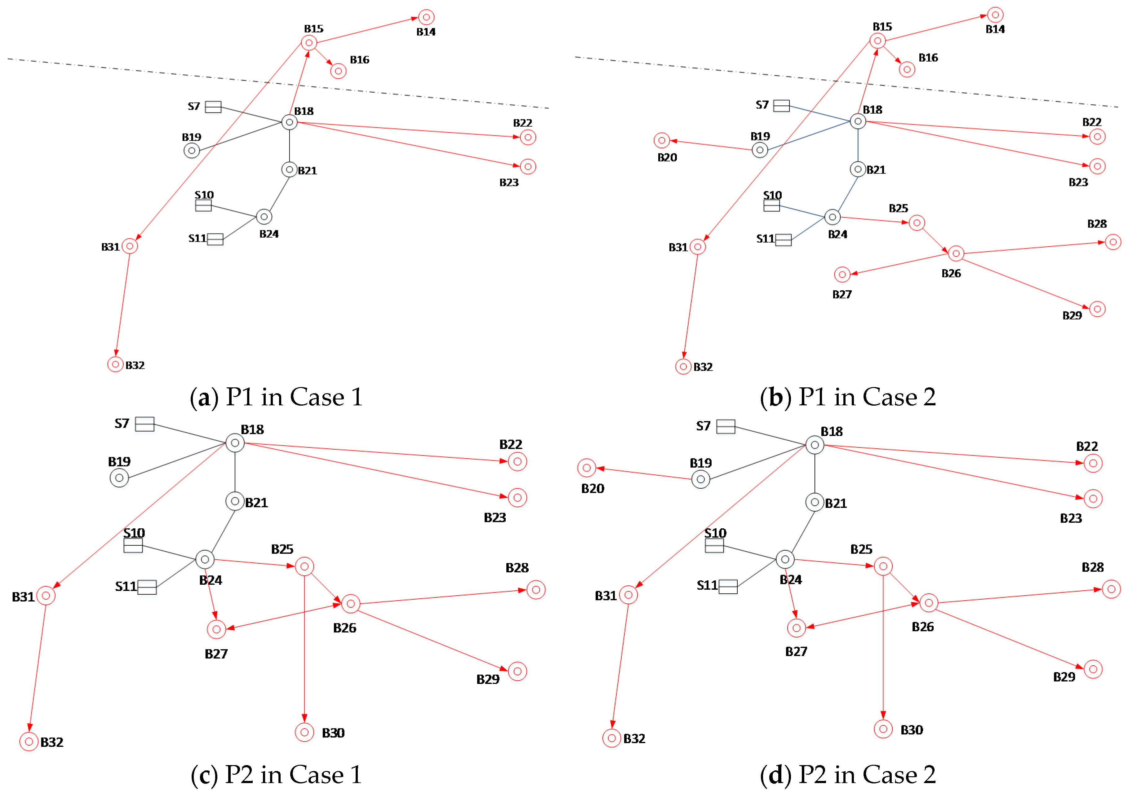
A non-sequential Monte-Carlo method is used for sampling, with a confidence level of 95%, and a total of 2400 states are extracted. The probability of system failure and the development of cascading faults are shown in Table 2 and Figure 7 in both cases.
The results of the analysis are as follows:
- (1)
- The system failure probability is low considering the protection malfunction, but the system interlocking fault is more serious, resulting in more serious load loss (more than 741,150 kW at P1 and 62,900 kW at P2). This shows that the protection hidden faults cause great harm to the system, which needs to be guarded against.
- (2)
- In P2, even in case 1, the source S12 can not complete the power supply in the remaining area because of the large-scale sources and line failure, which leads to large-scale line overload and large-scale transfer of power flow, so that the power system lost the heavy load, The entire southern region falls into a state of collapse; In P1, although the cascading fault spread to the northern region (B18 → B15 → B14 (B16)), which results in a partial loss. However, the tie line of B16–B25 is not affected, which ensures network operation and supports the southern power grid. The tie-line and S12 together provide power to the remaining grid and reduce losses.
- (3)
- From the development of chain failure, the stability of P1 is superior to that of P2. Quantitative evaluation results are shown in the following section.
4.3. Risk Assessment Results
As can be seen from the previous Section 3.2, the chain failure is more serious considering the protection hidden faults, so this section considers Case 2 for analysis.
Set the number of chain failure stages to day 1, after calculating the single risk index, the structural comprehensive risk, the failure comprehensive risk and economic loss risk are calculated by Formulas (16)–(20). The various types of risk indicators after the chain failure are shown in Table 3.
The results of the analysis are as follows:
- (1)
- From the structural risk value point of view: as there are more UHV lines in P1, resulting in an ALL value higher than P2. The MISCR of the two schemes are both more than 3.0, which belong to the strong short-circuit ratio level, but the value of P1 is higher than the value of P2, which indicates that the B15–B33 DC access scheme is better.
- (2)
- From the fault indicators and power loss point of view, P1 is obviously superior to P2, which indicates that, in this kind of accident state, due to the strong inter-regional AC/DC link, the large-scale power flow transfer caused by the power gap can be reasonably shared, so that the southern power grid gets strong support. Compared with P2, in the event of the same serious failure, P1 can lose less load.
The risk indicators for the recovery phase are calculated by days, until the system returns to full power. Since it is assumed that there is no new fault in the recovery phase, that is, the present probability is 1 and the new failure probability is 0. Thus, the comprehensive risk value is not calculated. Finally, the system structure indicators and failure indicators take the average value, and the power loss takes the cumulative value. The various indicators for the recovery phase are shown in Table 4.
Comparing Table 3 and Table 4, it can be seen that, during the recovery phase, all kinds of risk indicators of the system are still not optimistic, and the outage loss is more serious than the chain failure stage. Therefore, the loss of the recovery stage should be fully considered. As the chain fault stage in P2 suffers more serious damage, resulting in a longer recovery period, the power loss is much higher than P1.
To sum up, the ability to withstand natural disasters under synchronous operation of the regional power grid is better than asynchronous operation, so P1 is recommended as the better planning scheme.
5. Conclusions
This paper presents a whole process risk analysis method applicable to UHV power grids. The following work is completed: (1) based on the BPA stabilization procedure and non-sequential Monte Carlo method, a fast fault probability calculation method is proposed, and the whole process risk assessment model is established; (2) we have established a complete set of risk assessment indicators to effectively evaluate the structural and operational performance of AC/DC hybrid power grids; and (3) we carry on a simulation of the chain failure of an actual UHV AC/DC power grid, which provides a reference for evaluating the risk level of grid fault and guaranteeing safe operation of grids.
Acknowledgments
This work was financially supported by the National Natural Science Foundation (51277067) and the Central University Foundation (2015XS03).
Author Contributions
Rishang Long and Jianhua Zhang designed the study, Rishang Long performed the experiments and wrote the paper, and Jianhua Zhang reviewed and edited the manuscript. All authors read and approved the manuscript.
Conflicts of Interest
The authors have no conflict of interest to declare.
References
- Xin, E.; Ju, Y.; Yuan, H. Development and application of a wireless sensor for space charge density measurement in an ultra-high-voltage, direct-current environment. Sensors 2016, 16, 1743. [Google Scholar] [CrossRef] [PubMed]
- Dobson, I.; Chen, J.; Thorp, J.S.; Newman, D.E. Examining criticality of blackouts in power system models with cascading events. In Proceedings of the 35th IEEE Hawaii International Conference on System Sciences, Maui, HI, USA, 5–8 January 2002.
- Kirschen, D.S.; Jayaweera, D.; Nedic, D.P.; Allan, R.N. A probabilistic indicator of system stress. IEEE Trans. Power Syst. 2004, 19, 1650–1657. [Google Scholar] [CrossRef]
- Kirschen, D.S.; Jayaweera, D. Comparision of risk-based and deterministic security assessments. IET Gener. Trans. Distrib. 2007, 1, 527–533. [Google Scholar] [CrossRef]
- Lin, W.-F.; Tang, Y.; Bu, G.-Q. Definition and application of short circuit ratio for multi-infeed AC/DC power systems. Proc. CSEE 2008, 28, 1–8. [Google Scholar]
- Kwon, K.-B.; Park, H.; Lyu, J.-K.; Park, J.-K. Cost analysis method for estimating dynamic reserve considering uncertainties in supply and demand. Energies 2016, 9, 845. [Google Scholar] [CrossRef]
- Li, J.; Yan, B.; Zhang, A.; Wu, Q.; Hao, J. Reliability research for UHVDC bipolar area DC protection system. Power Syst. Prot. Control 2016, 44, 130–136. [Google Scholar]
- Ye, G.H.; Zhang, Y.; Zhang, Z.Q. A modified self-organized criticality method for power system risk assessment concerning influences of ultra-high-voltage transmission lines. Autom. Electr. Power Syst. 2015, 39, 44–52. [Google Scholar]
- Vaiman, M.; Bell, K.; Chen, Y.; Chowdhury, B.; Dobson, I.; Hines, P.; Zhang, P. Risk assessment of cascading outages: Methodologies and challenges. IEEE Trans. Power Syst. 2012, 27, 631–641. [Google Scholar] [CrossRef]
- Guo, L.; Guo, C.X.; Tang, W.H.; Wu, Q.H. Evidence-based approach to power transmission risk assessment with component failure risk analysis. IET Gener. Transm. Distrib. 2012, 7, 665–672. [Google Scholar] [CrossRef]
- Liu, Z.; Jia, H.J.; Xu, T.; Zeng, Y. Study on N-k risk based grid-connection and capacity allocation of wind farm and energy storage system. Power Syst. Technol. 2014, 38, 889–894. [Google Scholar]
- Nur, A.S.; Muhammad, M.O.; Mohd, S.S. Risk assessment of cascading collapse considering the effect of hidden failure. In Proceedings of the IEEE International Conference on Power and Energy, Kota Kinabalu, Malaysia, 2–5 December 2012.
- Tamronglak, S. Analysis of Power System Disturbances due to Relay Hidden Failures; Virginia Polytechnic and State University: Blacksburg, VA, USA, 1994. [Google Scholar]
- Zhao, H.; Li, N. Risk evaluation of a UHV power transmission construction project based on a cloud model and FCE method for sustainability. Sustainability 2015, 7, 2885–2914. [Google Scholar] [CrossRef]
- He, H.; Guo, J. Seismic disaster risk evaluation for power systems considering common cause failure. Proc. CSEE 2012, 28, 44–56. [Google Scholar]
- Li, W. Risk Assessment of Power Systems; IEEE Press & John Wiley & Sons, Inc.: New York, NY, USA, 2005. [Google Scholar]
- Cuadra, L.; Salcedo-Sanz, S.; Del Ser, J.; Jiménez-Fernández, S.; Geem, Z.W. A critical review of robustness in power grids using complex networks concepts. Energies 2015, 8, 9211–9265. [Google Scholar] [CrossRef] [Green Version]
- De Boer, P.-T.; Kroese, D.P.; Mannor, S.; Rubinstein, R.Y. A tutorial on the cross-entropy method. Ann. Oper. Res. 2005, 134, 19–67. [Google Scholar] [CrossRef]
Figure 1.
Development of chain failure.
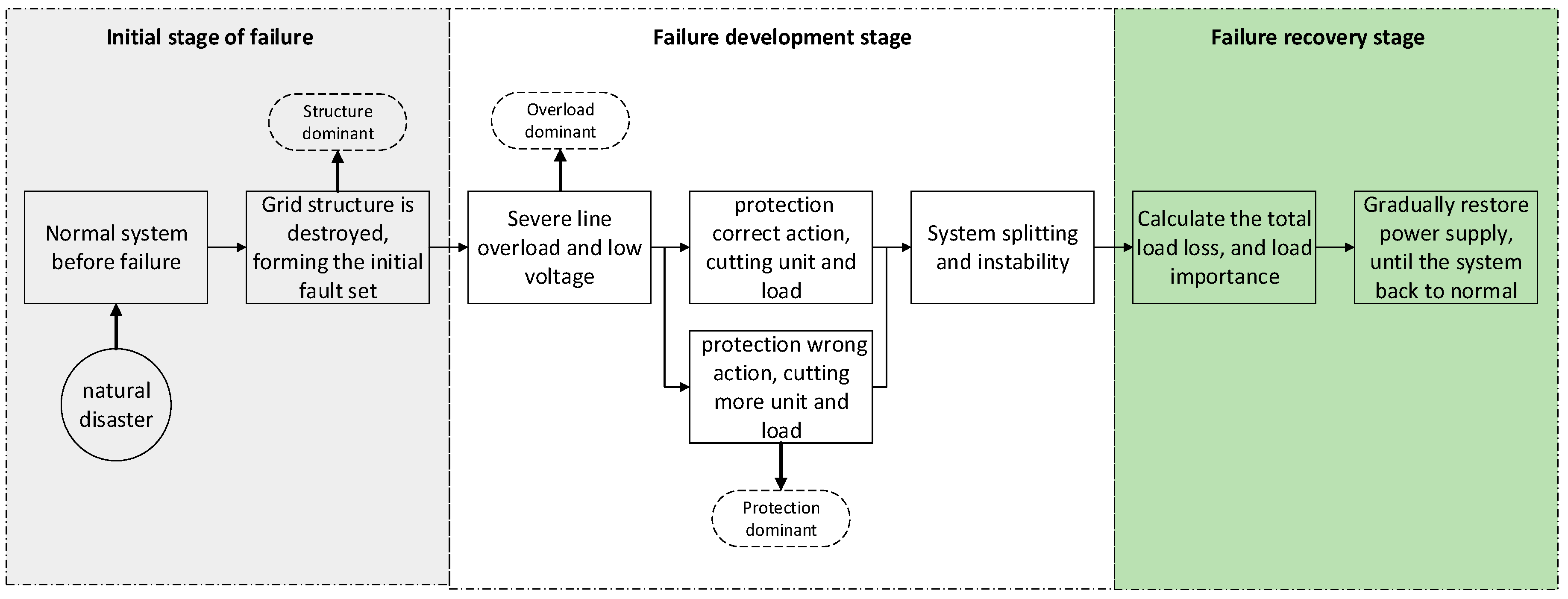
Figure 2.
Low voltage severity (LVS) function.
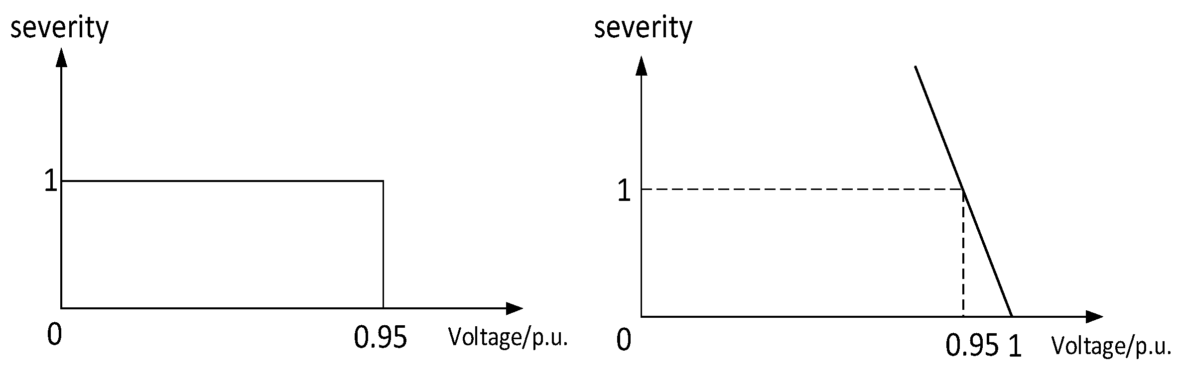
Figure 3.
Power angle difference severity (PADS) function.
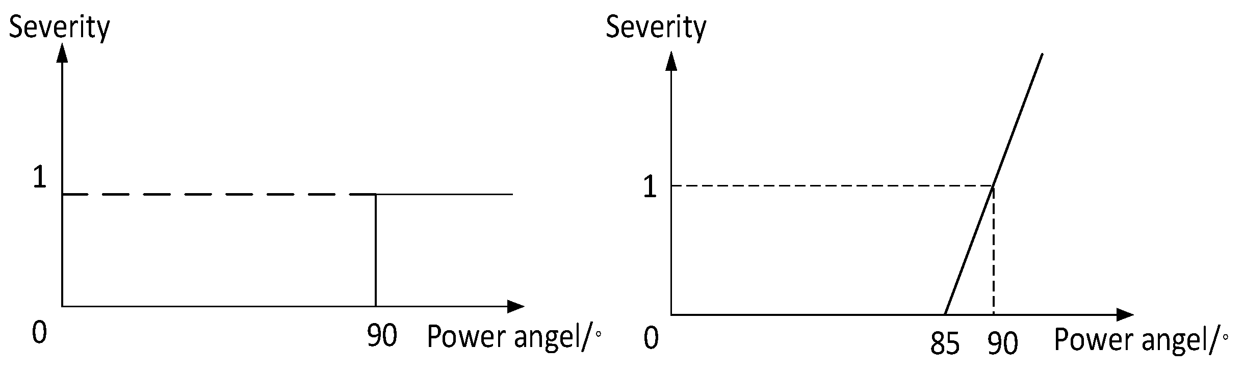
Figure 4.
System frequency severity (SFS) function.

Figure 5.
The calculation flow.

Figure 6.
Planning scheme for a regional grid. (a) Planning scheme 1; (b) Planning scheme 2.

Figure 7.
The development of cascading faults. (a) P1 in Case 1; (b) P1 in Case 2; (c) P2 in Case 1; (d) P2 in Case 2.
Figure 7.
The development of cascading faults. (a) P1 in Case 1; (b) P1 in Case 2; (c) P2 in Case 1; (d) P2 in Case 2.

| Classification | Indicators |
|---|---|
| System Structure | Average length of line (ALL) |
| Network average medians (NAM) | |
| Network average degrees (NAD) | |
| Multi-infeed short-circuit ratio (MISCR) | |
| Fault State | Low voltage severity (LVS) |
| Power angle difference severity (PADS) | |
| System frequency severity (SFS) | |
| Economic Losses | Power loss (PL) |
| Case 1 | Case 2 | ||
|---|---|---|---|
| Probability of Failure | P1 | 0.3914 | 0.0979 |
| P2 | 0.3909 | 0.0978 | |
| Chain Failure Process | P1 | B18 → B15 → B14 (B16), B18 → B22 (B23), B15 → B31 → B32 | B19 → B20, B18 → B15 → B14 (B16), B18 → B22 (B23), B15 → B31 → B32, B24 → B25 → B26 → B28 (B27, B29) |
| P2 | B18 → B22 (B23), B25 → B26 → B28 (B27, B29), B24 → B27, B24 → B25 → B30, B18 → B31 → B32 | B19 → B20, B18 → B22 (B23), B25 → B26 → B28 (B27, B29), B24 → B27, B24 → B25 → B30, B18 → B31 → B32 | |
| Loss of Load (MW) | P1 | 783.76 | 1524.91 |
| P2 | 1683.20 | 1746.18 |
| Index | P1 | P2 |
|---|---|---|
| ALL (km) | 742.14 | 730.28 |
| NAD | 2.54 | 2.41 |
| NAM | 1.33 | 1.30 |
| MISCR | 5.05 | 4.78 |
| structural comprehensive risk | 0.307 | 0.343 |
| LVS | 1.57 | 1.98 |
| PADS | 29.20 | 34.51 |
| SFS | 1.80 | 2.02 |
| failure comprehensive risk | 0.694 | 0.866 |
| PL (ten thousand yuan) | 914.96 | 1047.08 |
| economic loss risk | 89.30 | 102.40 |
| Index | P1 | P2 |
|---|---|---|
| ALL (km) | 749.25 | 732.77 |
| NAD | 2.58 | 2.53 |
| NAM | 1.48 | 1.48 |
| MISCR | 6.25 | 6.01 |
| LVS | 1.36 | 1.58 |
| PADS | 10.96 | 15.91 |
| SFS | 0.51 | 0.52 |
| PL (ten thousand yuan) | 1862.15 | 2635.58 |
© 2016 by the authors; licensee MDPI, Basel, Switzerland. This article is an open access article distributed under the terms and conditions of the Creative Commons Attribution (CC-BY) license (http://creativecommons.org/licenses/by/4.0/).
Share and Cite
MDPI and ACS Style
Long, R.; Zhang, J. Risk Assessment Method of UHV AC/DC Power System under Serious Disasters. Energies 2017, 10, 13. https://doi.org/10.3390/en10010013
AMA Style
Long R, Zhang J. Risk Assessment Method of UHV AC/DC Power System under Serious Disasters. Energies. 2017; 10(1):13. https://doi.org/10.3390/en10010013
Chicago/Turabian StyleLong, Rishang, and Jianhua Zhang. 2017. "Risk Assessment Method of UHV AC/DC Power System under Serious Disasters" Energies 10, no. 1: 13. https://doi.org/10.3390/en10010013
Note that from the first issue of 2016, this journal uses article numbers instead of page numbers. See further details here.