Article

Dependency Relations among International Stock Market Indices

by
Leonidas Sandoval Junior
1,*,
Asher Mullokandov
2 and
Dror Y. Kenett
3
1
Insper Instituto de Ensino e Pesquisa, Rua Quatá, 300, São Paulo, SP, 04546-042, Brazil
2
Department of Physics, Boston Univeristy, 590 Commonwealth Ave, Boston, MA 02215, USA
3
Center for Polymer Studies and Department of Physics, 590 Commonwealth Avenue, Boston, MA 02215, USA
*
Author to whom correspondence should be addressed.
J. Risk Financial Manag. 2015, 8(2), 227-265; https://doi.org/10.3390/jrfm8020227
Submission received: 1 December 2014 / Revised: 20 April 2015 / Accepted: 29 April 2015 / Published: 29 May 2015

Abstract

:
We develop networks of international stock market indices using information and correlation based measures. We use 83 stock market indices of a diversity of countries, as well as their single day lagged values, to probe the correlation and the flow of information from one stock index to another taking into account different operating hours. Additionally, we apply the formalism of partial correlations to build the dependency network of the data, and calculate the partial Transfer Entropy to quantify the indirect influence that indices have on one another. We find that Transfer Entropy is an effective way to quantify the flow of information between indices, and that a high degree of information flow between indices lagged by one day coincides to same day correlation between them.
JEL classifications:
G1; G15

1. Introduction

The world’s financial markets form a complex, dynamic network in which individual markets interact with one another. This multitude of interactions can lead to highly significant and unexpected effects, and it is vital to understand precisely how various markets around the world influence one another. Understanding how international financial market crises propagate is of great importance for the development of effective policies aimed at managing their spread and impact.
There is an abundance of work dealing with networks in finance, most of them concentrating on the interbank market. Seminal early work in this field is due to Allen and Gale [1] and subsequent studies are too numerous to cite here (for a list of theoretical and empirical studies, see [2] and references therein). These studies usually consider networks of banks with link assignment determined by borrowing and lending. Networks are built according to different topologies-such as random, small world, or scale-free-and the propagation of defaults through the network is studied. An important empirical observation is that these networks exhibit a core-periphery structure, with a few banks occupying central, more connected positions, and others populating a less connected neighborhood. Moreover, small world or scale-free networks are, in general, more robust to cascades (the propagation of shocks) than random networks, but they are also more prone to the propagation of crises if the most central nodes, usually those with more connections, are not themselves backed by sufficient funds. Another important finding is that the network structures changed considerably after the crisis of 2008, with a reduction of the number of connected banks and a more robust topology against the propagation of shocks.
There are many works that deal with international financial markets and their relations to one another, and most of these are based on correlation (see [3,4] and references therein). Since modern portfolios look for diversification of risk by incorporating stocks from foreign markets, it is important to understand when and how crises propagate across markets. Correlation is non causal and symmetric and is, therefore, not able to probe this question in detail.
In this work, we overcome part of this limitation by using two non-symmetric measures to study the dependency structure of global stock market indices, as defined in [5]. The first is Transfer Entropy [6], an information based measure that quantifies the flow of information from a source to a destination-stock market indices in our case; Transfer Entropy can be thought of as a measure of the reduction in uncertainty about future states of the destination variable due to past states of the source variable. Transfer Entropy is also model-independent and is sensitive to non-linear underlying dynamics, unlike, for example, Granger causality [7], to which Transfer Entropy is reduced for auto-regressive processes [8]. Transfer Entropy has been applied to the theory of cellular automata, to the study of the human brain, to the social media, to statistics, and to financial markets [9,10,11,12,13,14,15,16,17,18,19,20] and [2].
We will also consider the total influence or dependency [5], which incorporates the effect of intermediate variables that can influence the correlation or information flow between source and destination. Total influence was developed by Kenett et al in order to compute and investigate the mutual dependencies between network nodes from the matrices of node-node correlations. The basis of this method is the partial correlations between a given set of variables (or nodes) of the network [5,21,22,23]. This new approach quantifies how a particular node in a network affects the links between other nodes, and is able to uncover important hidden information about the system. While this method has been mainly developed for the analysis of financial data, it was recently applied to the investigation of the immune system [24] and to semantic networks [25]. We incorporate the dependency network approach with Transfer Entropy to identify and represent causal relations among financial markets.
Our data consists of 83 stock market indices, and their values lagged by one day, belonging to 82 countries. We calculate the same-day and previous-day correlation and Transfer Entropy for the 83 indices, and construct the dependency networks with correlation and Transfer Entropy as network edges. We then show the representation of the correlation and effective Transfer Entropy dependency networks in terms of a distance measure between indices. Additionally, we discuss network centralities based on the resulting networks, and rank the most strongly influencing nodes of our network. Finally, we study the dynamics of the two networks portrayed in the previous sections, and compare the changes in average correlation and Transfer Entropy dependency to the average volatility during the same period.
Section 2 of this article discusses the choice of data and how it was treated; Section 3 shows both theory and results for correlation, Transfer Entropy, and effective Transfer Entropy. Section 4 discusses dependency networks and shows results for our set of data; Section 5 builds network representations based on influence networks built from correlation and effective Transfer Entropy; Section 6 discusses the centralities of the indices according to complex network theory. Section 7 brings a discussion of the methods applied to data based on the volatilities of the indices, and Section 8 presents our conclusions.

2. The Data

The data we use are based on the daily closing values of the benchmark indices of 83 stock markets around the world from January 2003 to December, 2014, collected from a Bloomberg terminal, spanning periods of both normal behavior and of crises in the international financial system. Two of the indices are of the US market (S&P 500 and Nasdaq), and each of the others is the benchmark index of the stock market of a different country. The names of the indices used and the countries they belong to may be found in Appendix A. The aim is to study a large variety of stock markets, both geographically and in terms of volume of negotiations.
Due to differences in national holidays and weekends, the working days of many of the indices vary. Removing all days in which any index wasn’t calculated would greatly reduce the size of the data, therefore our approach, similar to what has been done in [3], was to remove only the days in which less than 60% of the stock markets did not operate. For markets that did not operate in one of the filtered days, we repeated the previous day’s value of its index. This approach deeply affected the indices of Israel, Jordan, Saudi Arabia, Qatar, the United Arab Emirates, Oman, and Egypt, which have different weekends than most of the other indices. For these countries, many operating days were removed. We ended up with an average of 93 ± 5 % (average plus or minus standard deviation) of markets operating on the same day.
An important aspect of international financial markets is that each individual market does not operate during the same hours. In [4], one of the present authors proposed a possible solution to this problem, which is to consider, in addition to the market indices, their one-day lagged counterparts. The lagged indices are treated as different variables and an enlarged correlation matrix is then built, containing both same-day and previous-day correlations. We calculate this enlarged matrix for the Transfer Entropy as well.
All calculations are made using the log-returns of prices, which suffer less with non-stationarity, and which are given by
R t = ln ( P t ) - ln ( P t - 1 )
where P t is the closing value of an index at day t and P t - 1 is the closing value of the same index at day t - 1 . We worked with the log-returns in order to avoid issues due to the nonstationarity of the time series of the closing values of the indices. All time series of log-returns are considered trend stationary by the Dickey-Fuller test [26], by the Augmented Dickey-Fuller test, and by the Phillips-Perron test [27]. About 59% of the time series fail the KPSS test for stationarity [28]. Only three of the time series (those of Iceland, Zambia, and Costa Rica) fail the Variance ratio test for random walk [29,30,31].

3. Correlation and Transfer Entropy
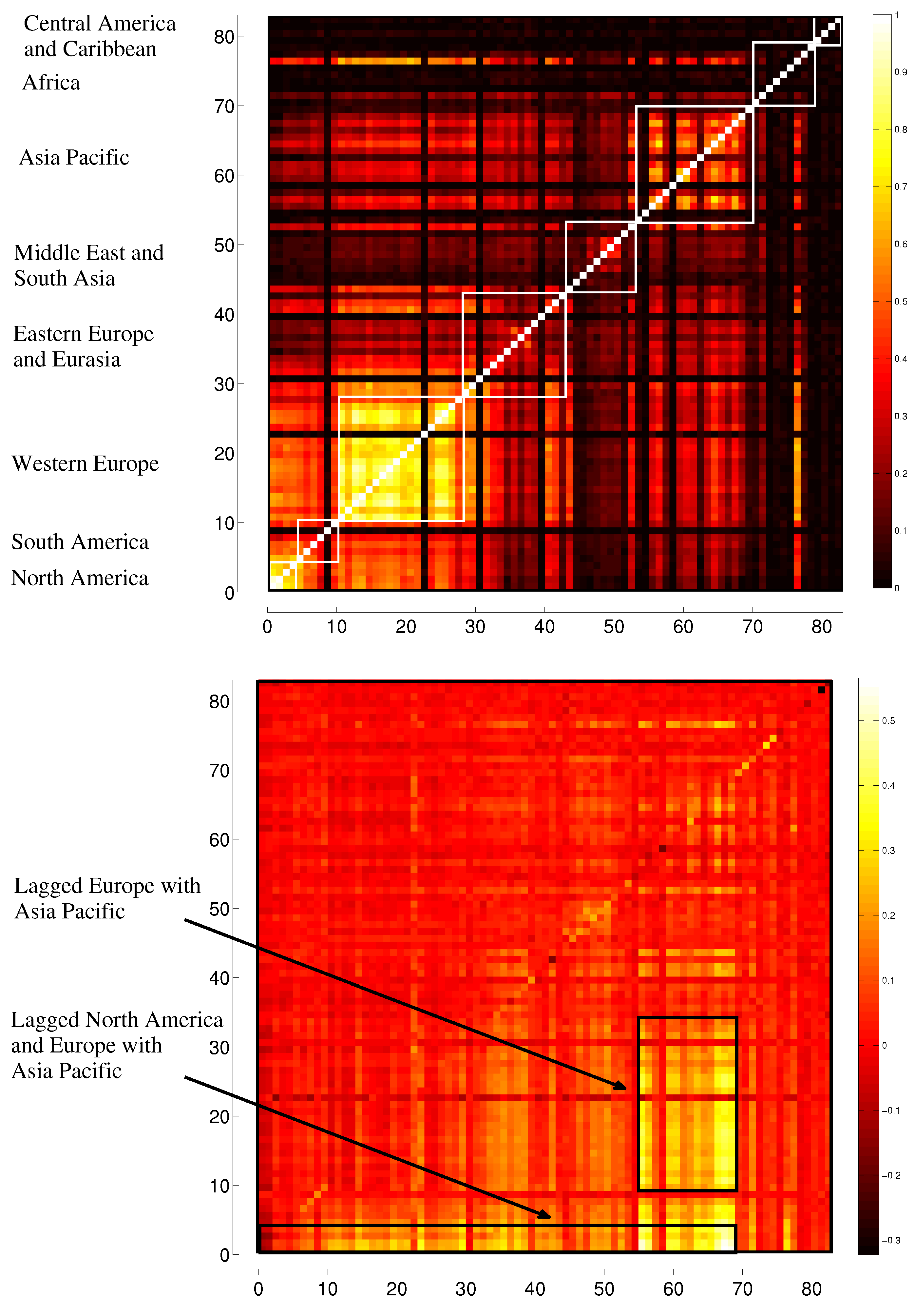
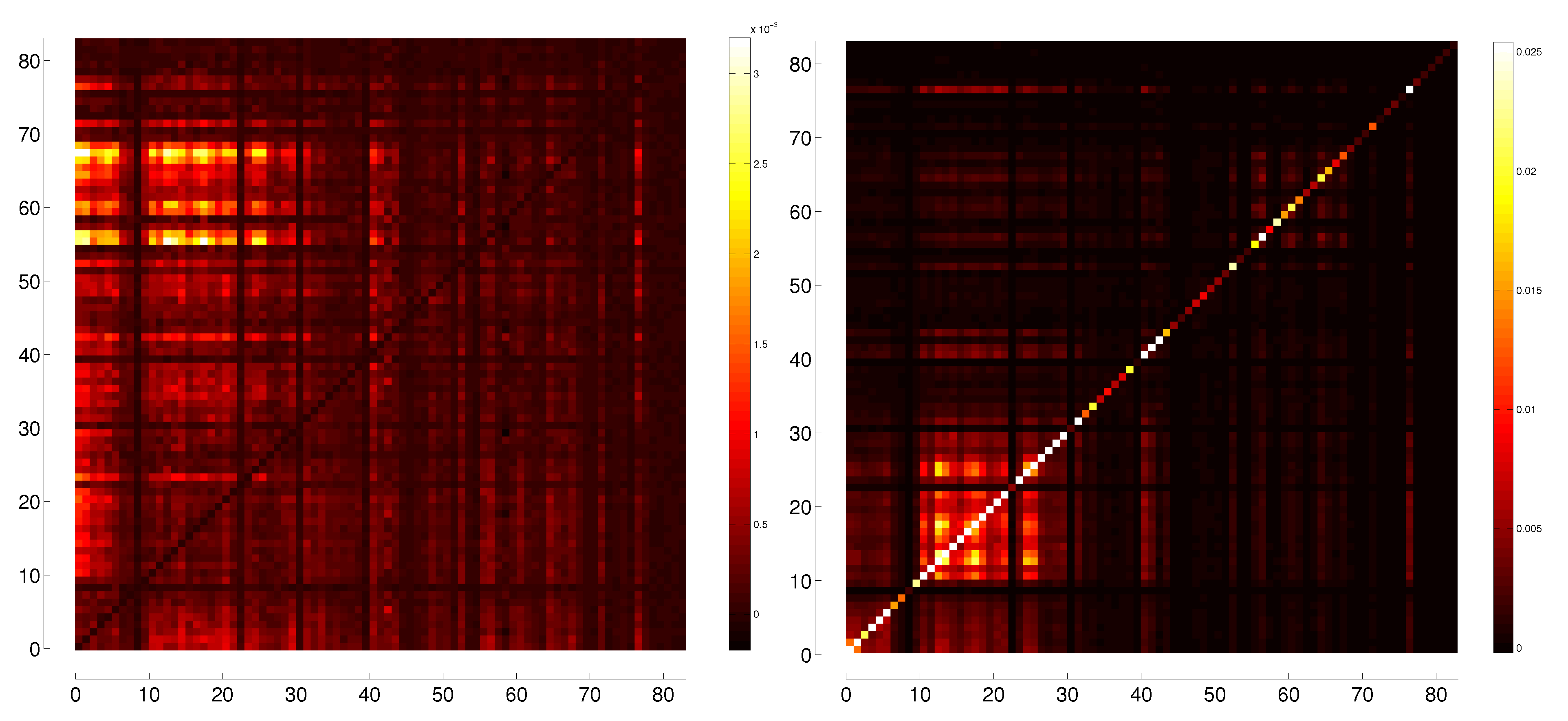
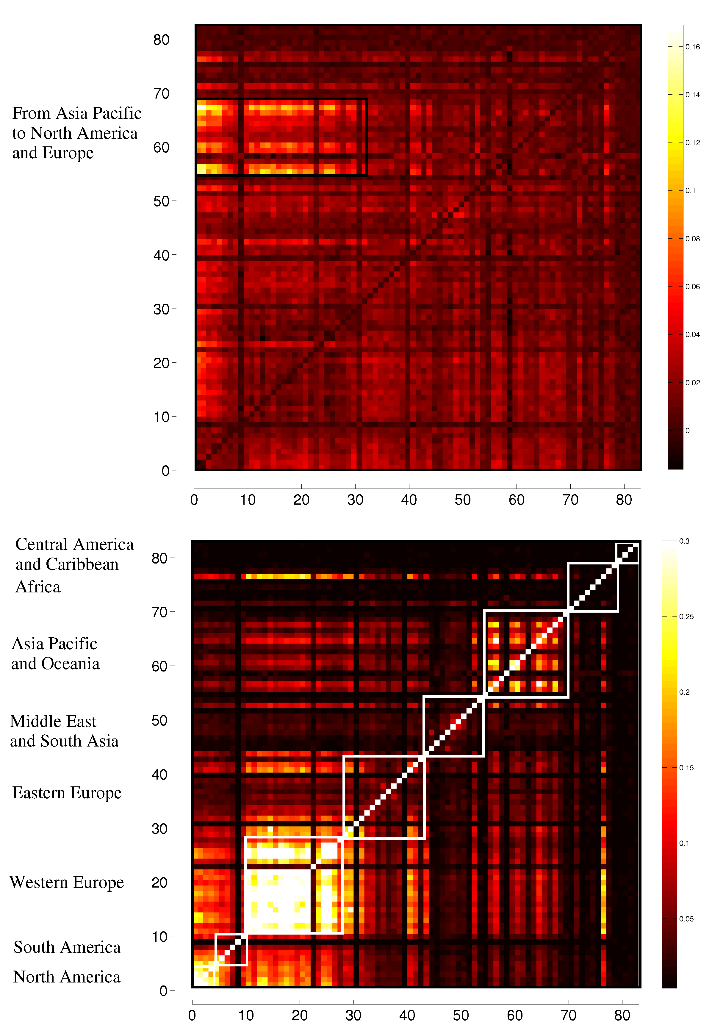
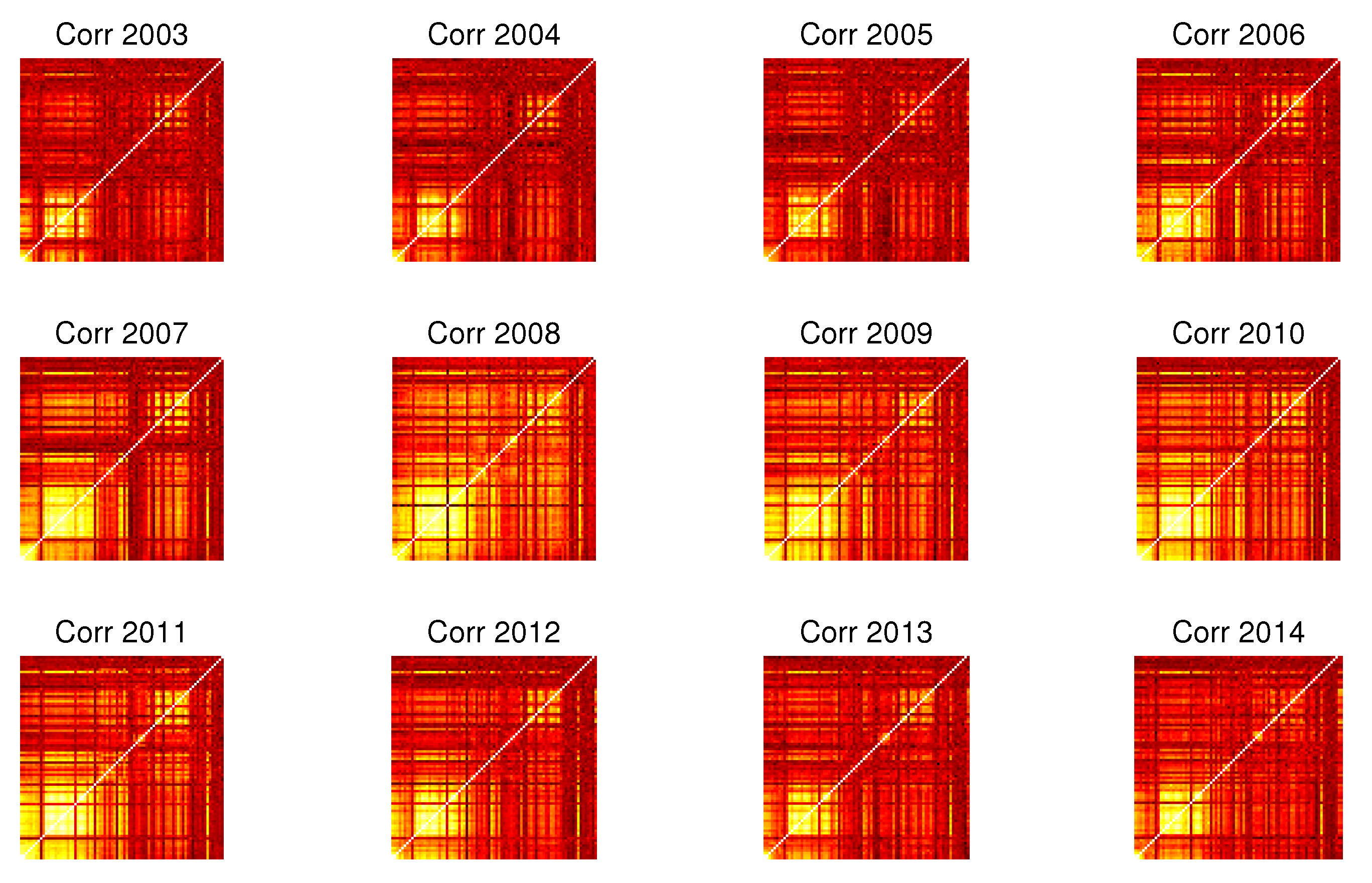
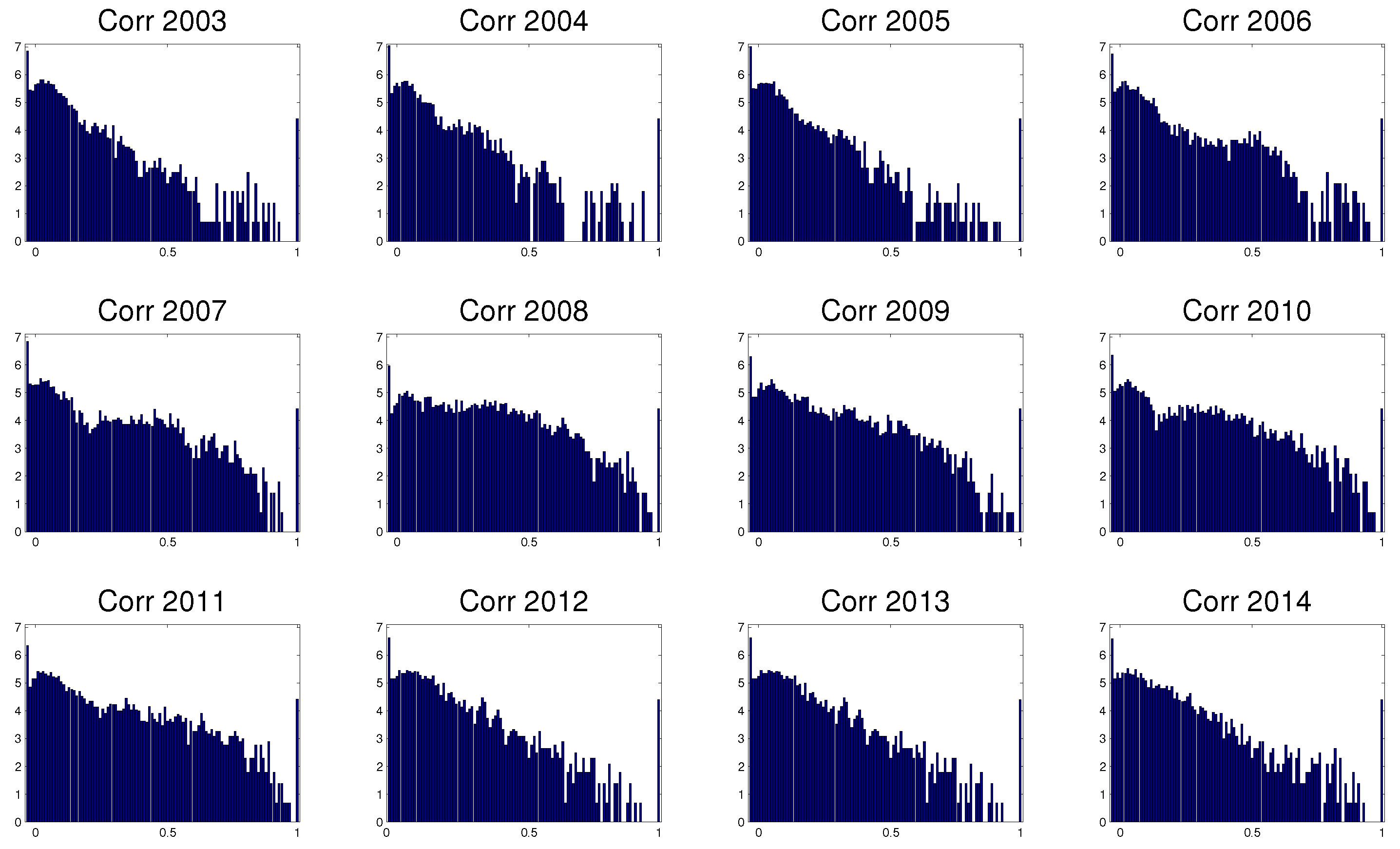
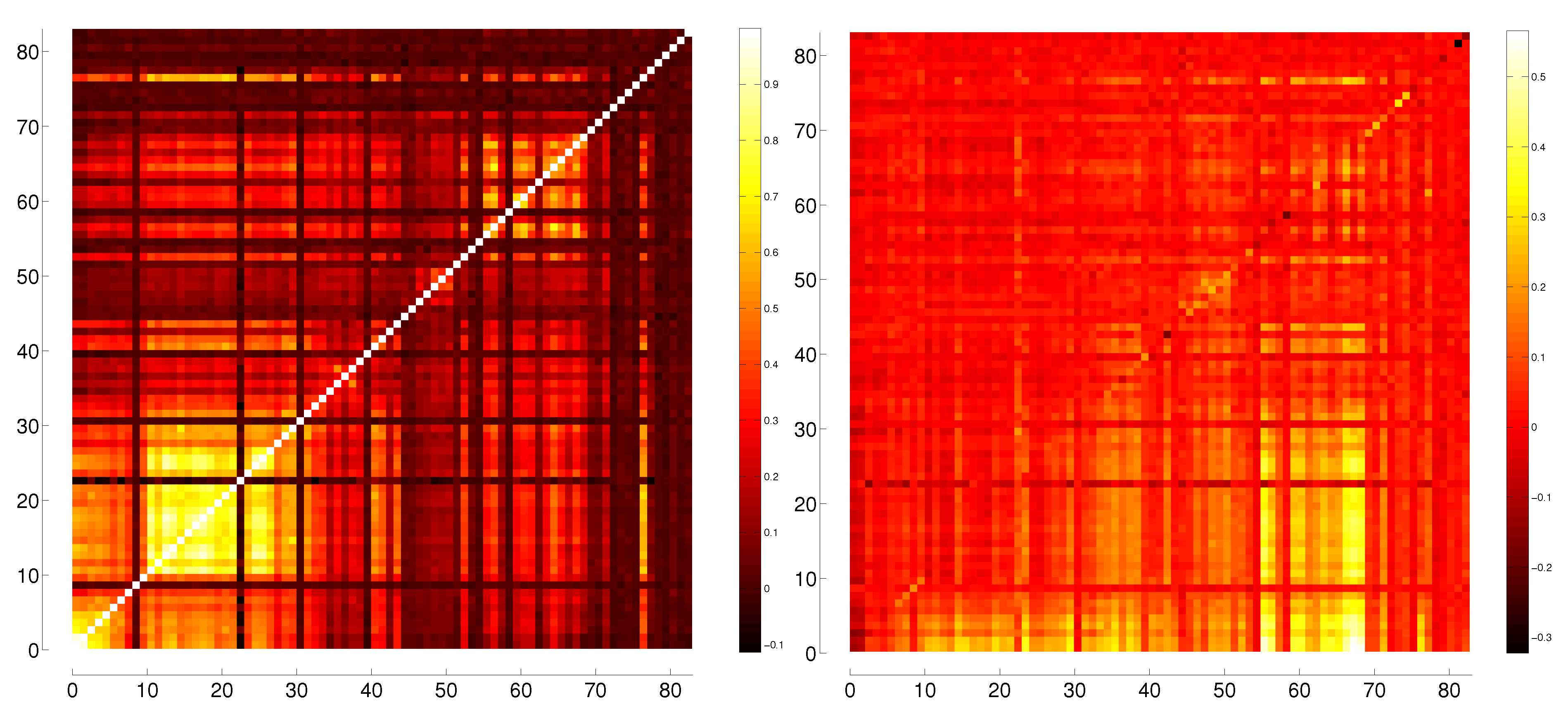
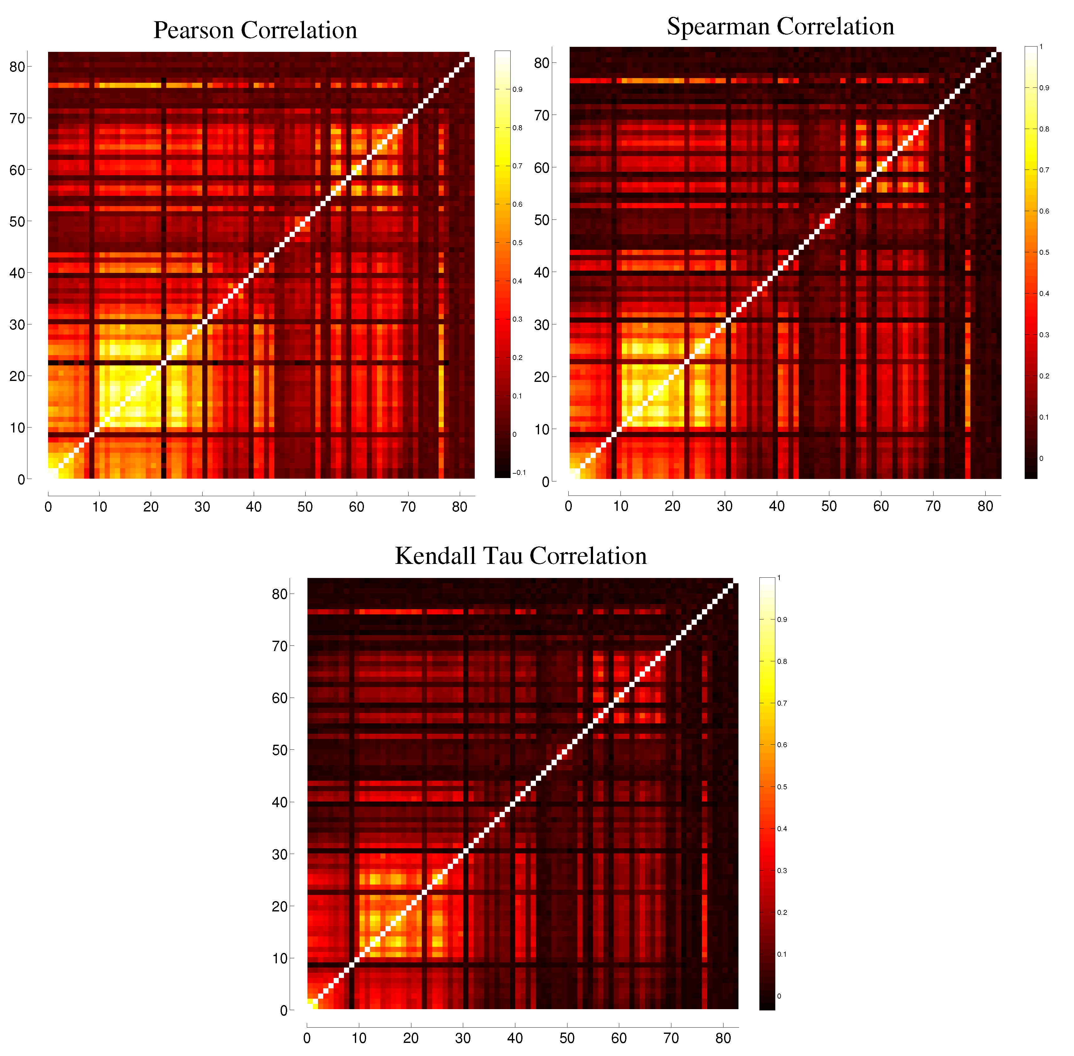
In this section, we calculate the correlation and Transfer Entropy matrices using the 83 indices previously described plus their lagged values.

3.1. Correlation

The Pearson correlation is given by
C i j = k = 1 n x i k - x i ¯ ) ( x j k - x j ¯ k = 1 n x i k - x i ¯ 2 k = 1 n x j k - x j ¯ 2
where x i k is element k of the time series of variable x i , x j k is element k of the time series of variable x j , and x i ¯ and x j ¯ are the averages of both time series, respectively.
Pearson correlation is used to calculate the linear correlation between variables. While other correlation measures, such as Spearman rank correlation and Kendall tau rank correlation, capture nonlinear relations, we apply the usual Pearson correlation because the results for the financial data we are using are very similar to the Spearman rank correlation, suggesting a near linear correlation between the indices. This discussion is made in Appendix B, where the three correlation measures are compared when applied to our set of data.
Using both original and lagged indices, we build a enlarged correlation matrix, displayed in Figure 1, with the original indices arranged from 1 to 83, and the lagged indices from 84 to 166. Enlarged correlation values are represented in lighter shades, and lower correlations are represented by darker shades.
Figure 1. Heat map of the enlarged correlation matrix of both original and lagged indices, representing same-day correlation in Sector 1 and previous-day correlation in Sector 2. Correlation is symmetric, therefore, Sectors 3 and 4 are identical to Sectors 1 and 2.
Jrfm 08 00227 g001
Figure 2 shows the magnified correlation submatrices of Sector 1 (left), the original indices with themselves, and Sector 2 (right), the lagged indices with the original ones. In Sector 1, where correlations go from - 0.1143 to 1, besides the bright main diagonal, representing the correlation of an index with itself, which is always 1, there are other clear regions of strong correlation-the North American, South American, and Western European indices all cluster regionally. There is a region of weaker correlation, among Asian countries and those of Oceania, and darker areas correspond to countries of Central America and some islands of the Atlantic. In Western Europe, the index of Iceland has very low correlation with the others, and African indices, with the exception of the one from South Africa, also interact weakly in terms of correlation. Other, off diagonal bright areas correspond to strong correlations between indices of the Americas and those of Europe, and weaker correlations between Western indices and their same-day counterparts in the East.
In Sector 2 of the correlation matrix, we see the correlations between lagged and original indices, that go from - 0.3227 to 0.5657 . Here, one can see some correlation between American and European indices and next day indices from Asia and Oceania, as well as some correlation between American indices and the next day values of European indices. This suggests an influence of West to East in terms of the behavior of the indices, which we will explore in more detail in later sections. There is little correlation between the lagged value of an index and its value on the next day.
Figure 2. Heat maps of the correlation submatrices for original × original indices and for lagged original indices, respectively.
Jrfm 08 00227 g002

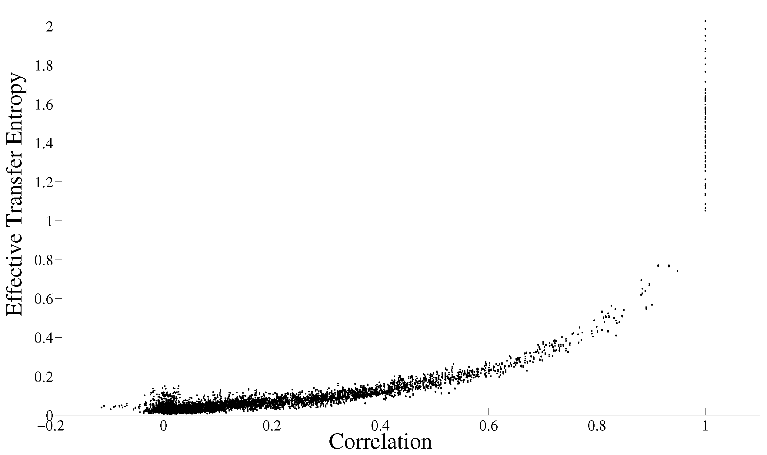
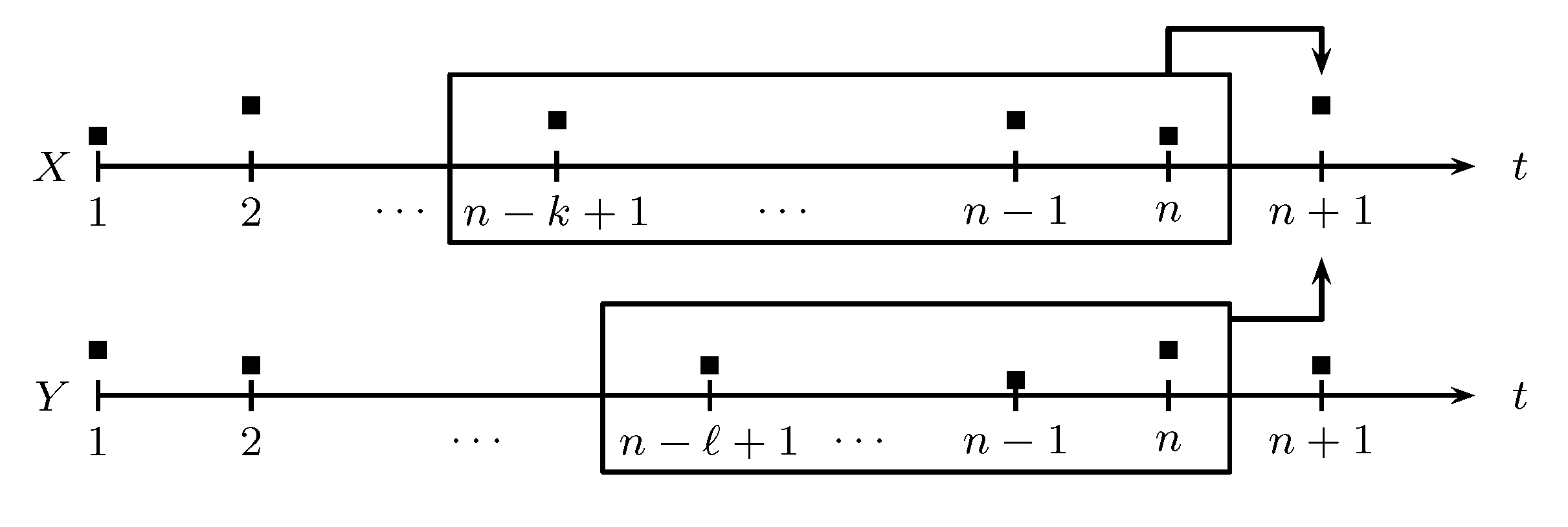
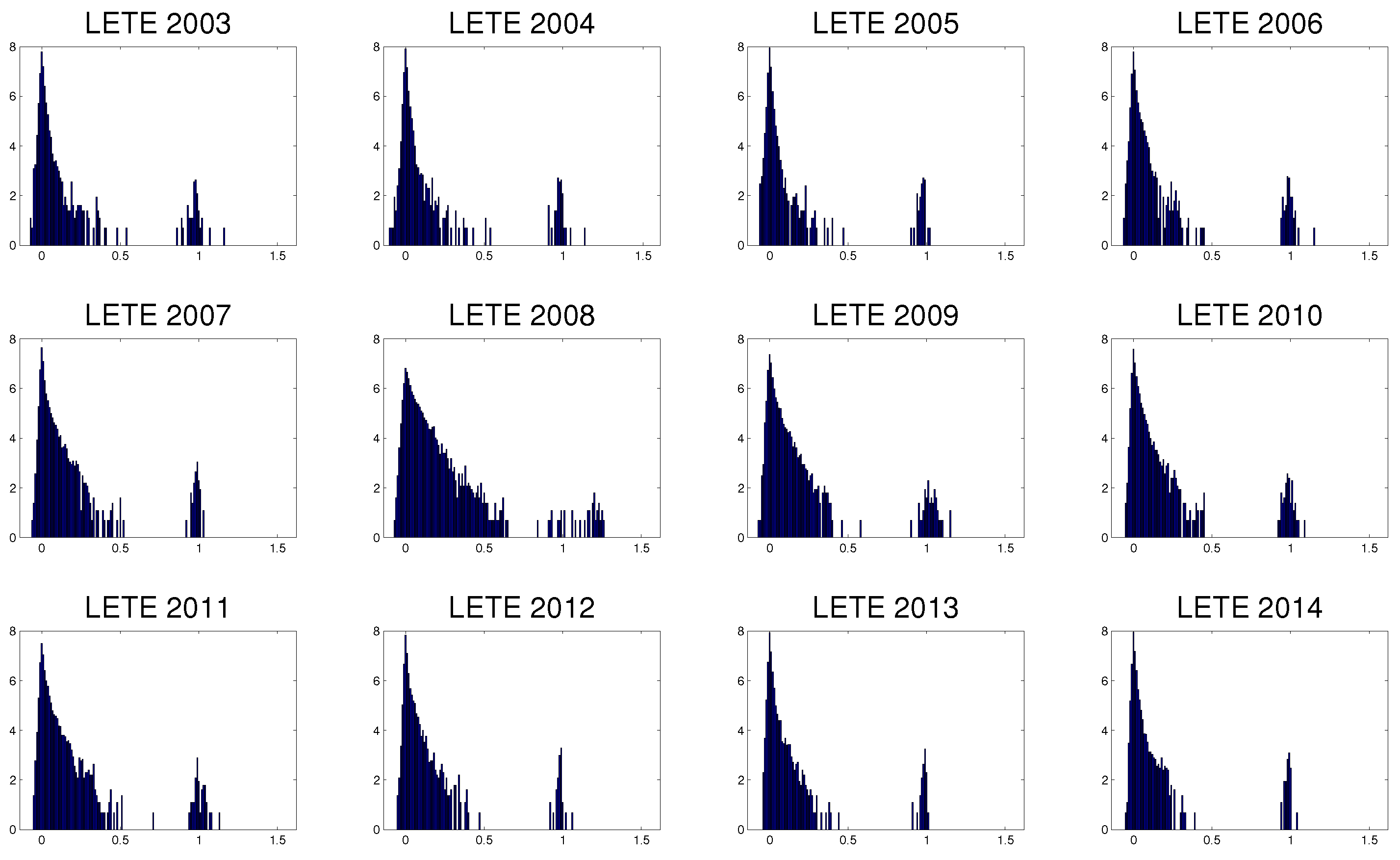
3.2. Transfer Entropy

To further explore the question of which markets influence others we turn to information based measures, in particular Transfer Entropy, that was created by Thomas Schreiber [6] as a measurement of the amount of information that a source sends to a destination. Such a measure must be asymmetric, since the amount of information that is transferred from the source to the destination need not, in general, be the same as the amount of information transferred from the destination to the source. It must also be dynamic-as opposed to mutual information which encodes the information shared between the two states. Transfer Entropy is constructed from the Shannon entropy [32], given by
H = - i = 1 N p i log 2 p i
where the sum is over all states for which p i 0 . The base 2 for the logarithm is chosen so that the measure of information is given in bits. This definition resembles the Gibbs entropy but is more general as it can be applied to any system that carries information.
Shannon entropy represents the average uncertainty about measurements i of a variable X, and quantifies the average number of bits needed to encode the variable X. In our case, given the time series of an index of a stock market ranging over a certain interval of values, one may divide the possible values into N different bins and then calculate the probabilities of each state i.
For interacting variables, time series may influence one another at different times. We assume that the time series of X is a Markov process of degree k, that is, a state i n + 1 of X depends on the k previous states of X:
p i n + 1 | i n , i n - 1 , , i 0 = p i n + 1 | i n , i n - 1 , , i n - k + 1
where p ( A | B ) is the conditional probability of A given B, defined as
p ( A | B ) = p ( A , B ) p ( B )
Modelling interaction between nodes, we also assume that state i n + 1 of variable X depends on the previous states of variable Y, as represented schematically in Figure 3.
Figure 3. Schematic representation of the Transfer Entropy between a variable Y and a variable X.
Jrfm 08 00227 g003
We may now define the Transfer Entropy from a time series Y to a times series X as the average information contained in the source Y about the next state of the destination X which was not already contained in the destination’s past. We assume that element i n + 1 of the time series of variable X is influenced by the k previous states of the same variable and by the previous states of variable Y:
Transfer Entropy from variable Y to variable X is defined as
T E Y X ( k , ) = = i n + 1 , i n ( k ) , j n ( ) p i n + 1 , i n ( k ) , j n ( ) log 2 p i n + 1 | i n ( k ) , j n ( ) - i n + 1 , i n ( k ) , j n ( ) p i n + 1 , i n ( k ) , j n ( ) log 2 p i n + 1 | i n ( k ) = i n + 1 , i n ( k ) , j n ( ) p i n + 1 , i n ( k ) , j n ( ) log 2 p i n + 1 | i n ( k ) , j n ( ) p i n + 1 | i n ( k )
where i n is element n of the time series of variable X and j n is element n of the time series of variable Y, p ( A , B ) is the joint probability of A and B, and
p i n + 1 , i n ( k ) , j n ( ) = p i n + 1 , i n , , i n - k + 1 , j n , , j n - + 1
is the joint probability distribution of state i n + 1 , of state i n and its k predecessors, and the predecessors of state j n , as in Figure 3.
This definition of Transfer Entropy assumes that events on a certain day may be influenced by events of k and previous days. We shall assume, with some backing from empirical data for financial markets, that only the previous day is important (ie, k = = 1 ). The Transfer Entropy Equation (6) then simplifies:
T E Y X = i n + 1 , i n , j n p i n + 1 , i n , j n log 2 p i n + 1 | i n , j n p i n + 1 | i n
In order to calculate Transfer Entropy using Equation (8), we must first establish a series of bins in which data may be fitted. The number of bins alter the resulting TE, and in order to gauge the effects of binning choice, in Appendix C, we calculated TE for our set of data for binnings with three different widths: 0.02 , 0.1 , and 0.5 . The results did not change substantially from one binning to the other, and since the heat maps from binning with width 0.02 were clearer, we adopted this binning in the remaining of our calculations.
Transfer Entropy, like other measures, is usually contaminated with noise due to finite data points, residual non-stationarity of data, etc. To reduce this contamination, we calculate the Transfer Entropy from randomized data, where time series are randomly reordered to destroy any correlation or causality relation between variables but to preserve their frequency distributions. The randomized data is then subtracted from the original Transfer Entropy matrix, producing the Effective Transfer Entropy (ETE), first defined in [9], and used in the financial setting by [2] and [20]. In the present work, we calculated ten Transfer Entropy matrices based on randomized data and then removed their average from the original Transfer Entropy matrix, obtaining the effective Transfer Entropy matrix presented in Figure 4. The heat map in Figure 4 are colored in such a way as to enhance visibility, so the largest brightness was set to 0.3 (so, every cell with ETE value above 0.3 is painted white) in order to make the figures more visible, although the range of values goes from –0.0203 to 1.8893.
The resulting ETE matrix is strikingly different from the correlation matrix. Here the ETEs from original to original indices, shows some weak flow from Asian Pacific and Oceanian indices to American and European indices, and from European indices to the American ones. Now, Sector 2, representing the ETEs from lagged to original indices, shows strong ETEs from the indices of one continent to the indices of the same continent on the next day, as can be seen by the brighter squares around the main diagonal of the quadrant. Off diagonal bright regions also show a flow of information from lagged American to European indices, from lagged European to Asian Pacific indices, and from lagged Asian Pacific to both American and European indices. Sector 3 mimics the ETEs of Sector 1, and Sector 4 features ETEs compatible with noise, which is to be expected since causality relations should not go backwards in time.
Sector 2 of the ETE matrix are the result of lagged Transfer Entropy by one day. In [33], the authors used lagged Transfer Entropy in order to study neuronal interaction delays, and [34] implements the calculation of a diversity of information-based measures, including the possibility of using lagged variables in TE.
Figure 4. Effective Transfer Entropy (ETE) matrix. Brighter areas correspond to large values of ETE, and darker areas correspond to low values of ETE.
Jrfm 08 00227 g004
Figure 5 shows close views of Sector 1 and Sector 2, respectively. From Sector 1, where ETE ranges from - 0.0162 to 0.1691 , one can see an ETE from Asian and Oceanian indices to American and European ones on the same day, indicating information flow from Asian and Oceanian markets to the West. Section 2 depicts the ETEs from lagged to original variables, ranging from 0.0185 to 1.8893 . There is a clear bright streak from lagged indices to themselves on the next day, which is to be expected given the definition of Transfer Entropy. We also see structures very similar to the ones obtained from Sector 1 of the correlation matrix, but now from lagged indices to original ones, leading to the belief that the flow of information from previous days anticipates correlation. There are clear clusters of North and South American indices, of Western European indices, and of Asian Pacific plus Oceanian indices. Although an ETE matrix need not be symmetric, the structure shown in Figure 5b is nearly symmetric, showing there is a comparable flow of information in both directions. Figure 5b has been colored so as to enhance visibility so that all values above 0.3 are represented as white.
Figure 2, left (Sector 1 of the correlation matrix), and Figure 5, right (Sector 2 of the ETE matrix), display a very similar structure, which suggests that the transfer of information from one index to another coincides to correlated behavior of the two indices on the following day. Figure 6 shows a plot of correlation values of the two submatrices. There is a clear nonlinear correlation between them: the Pearson (linear) correlation between them is 0.73, the Spearman rank correlation between them is 0.82, and the Kendall tau rank correlation between them is 0.66.
Figure 5. Heat maps of the ETE submatrices from original to original indices and from lagged to original indices, respectively.
Jrfm 08 00227 g005
Figure 6. Correlation values of Sector 1 of the correlation matrix and Effective Transfer Entropy (ETE) of Sector 2 of the ETE matrix.
Jrfm 08 00227 g006

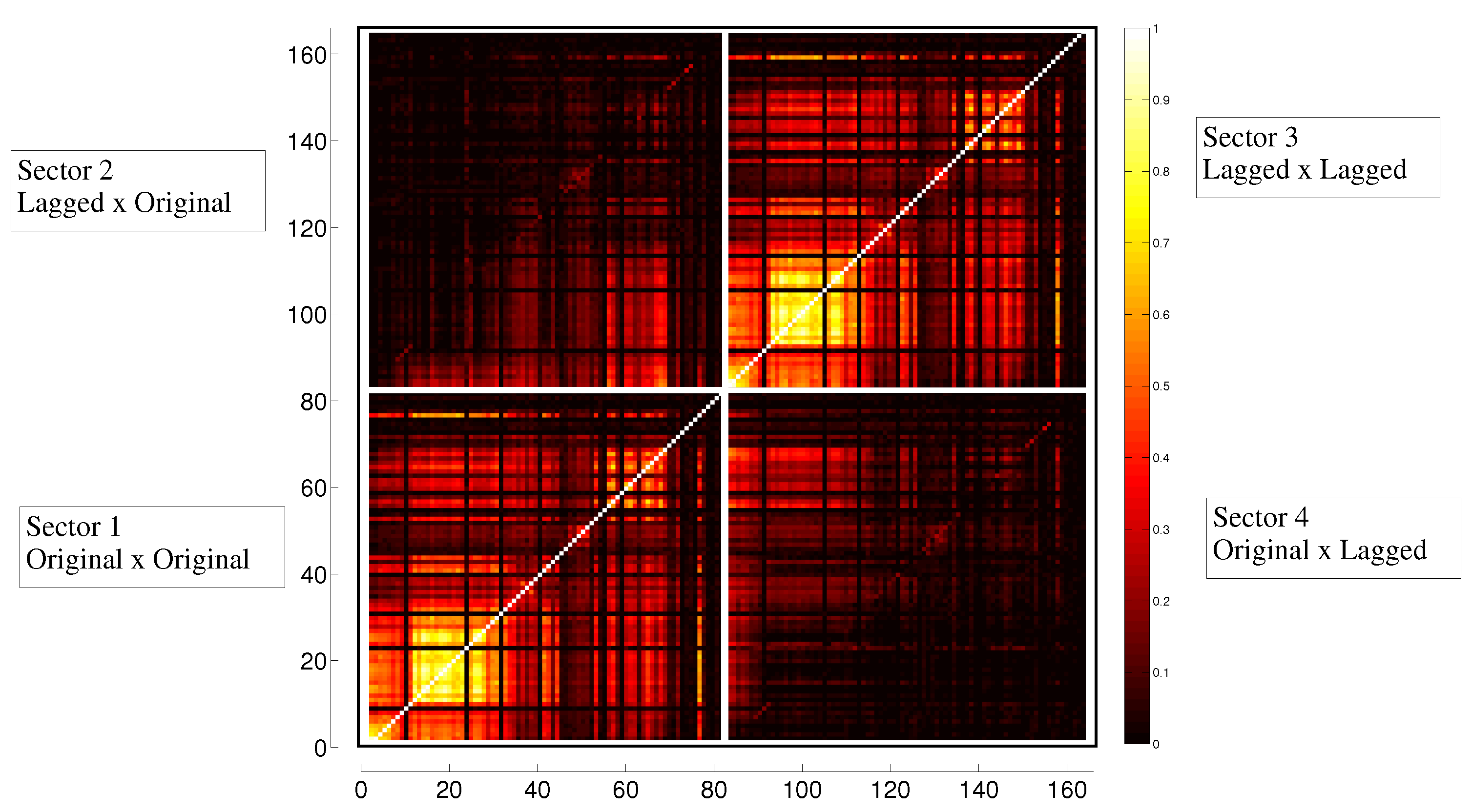
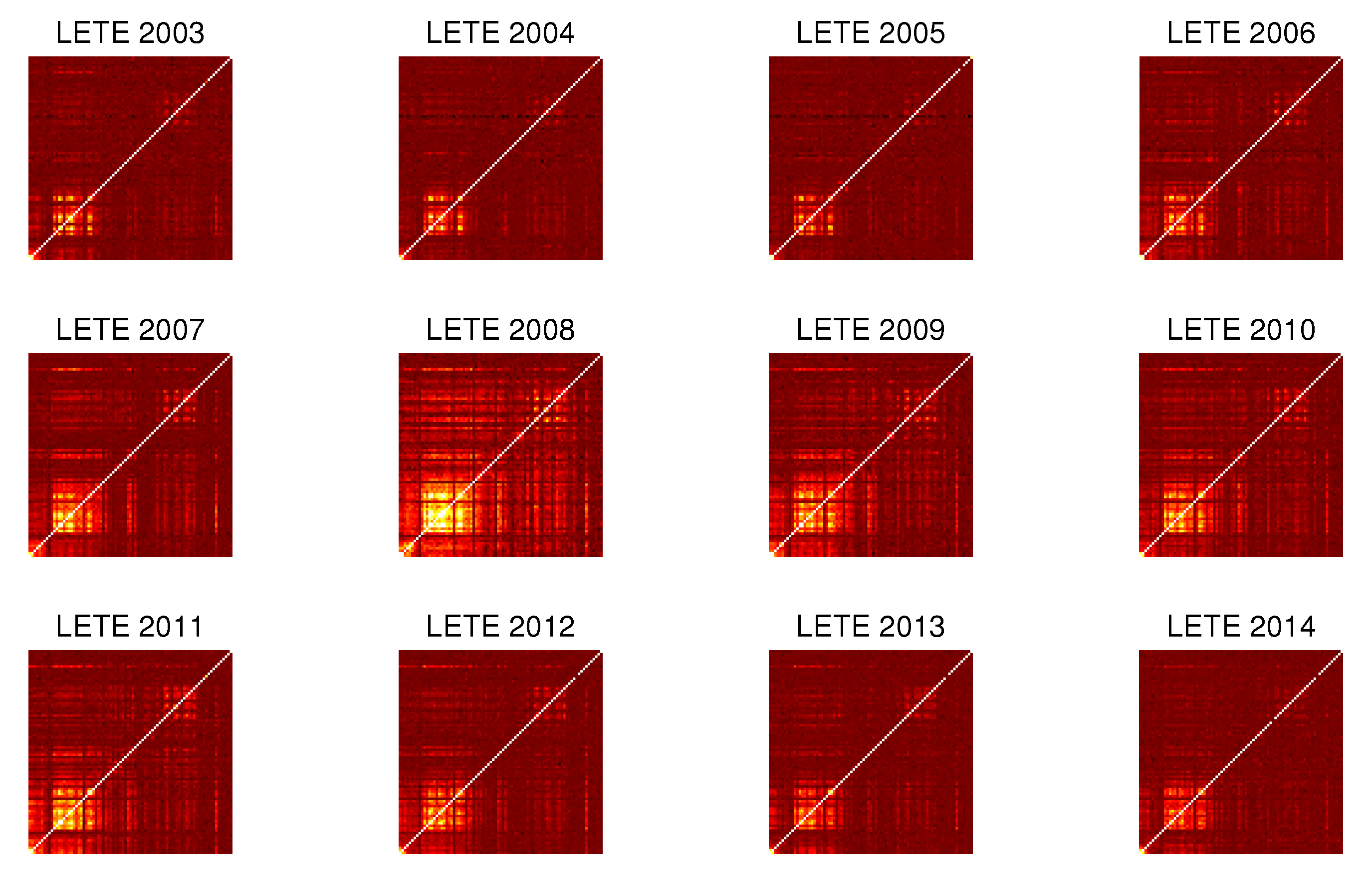
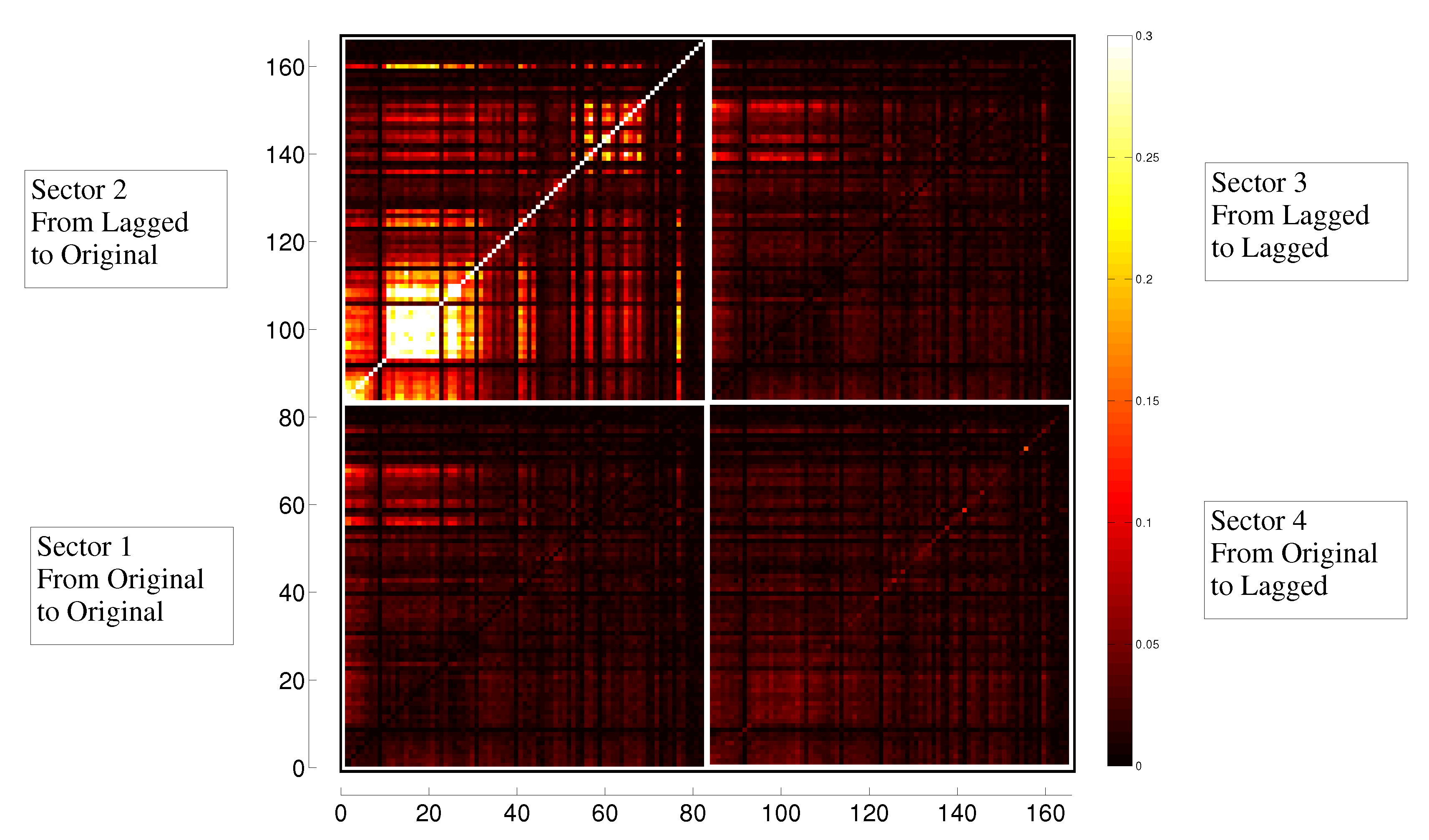
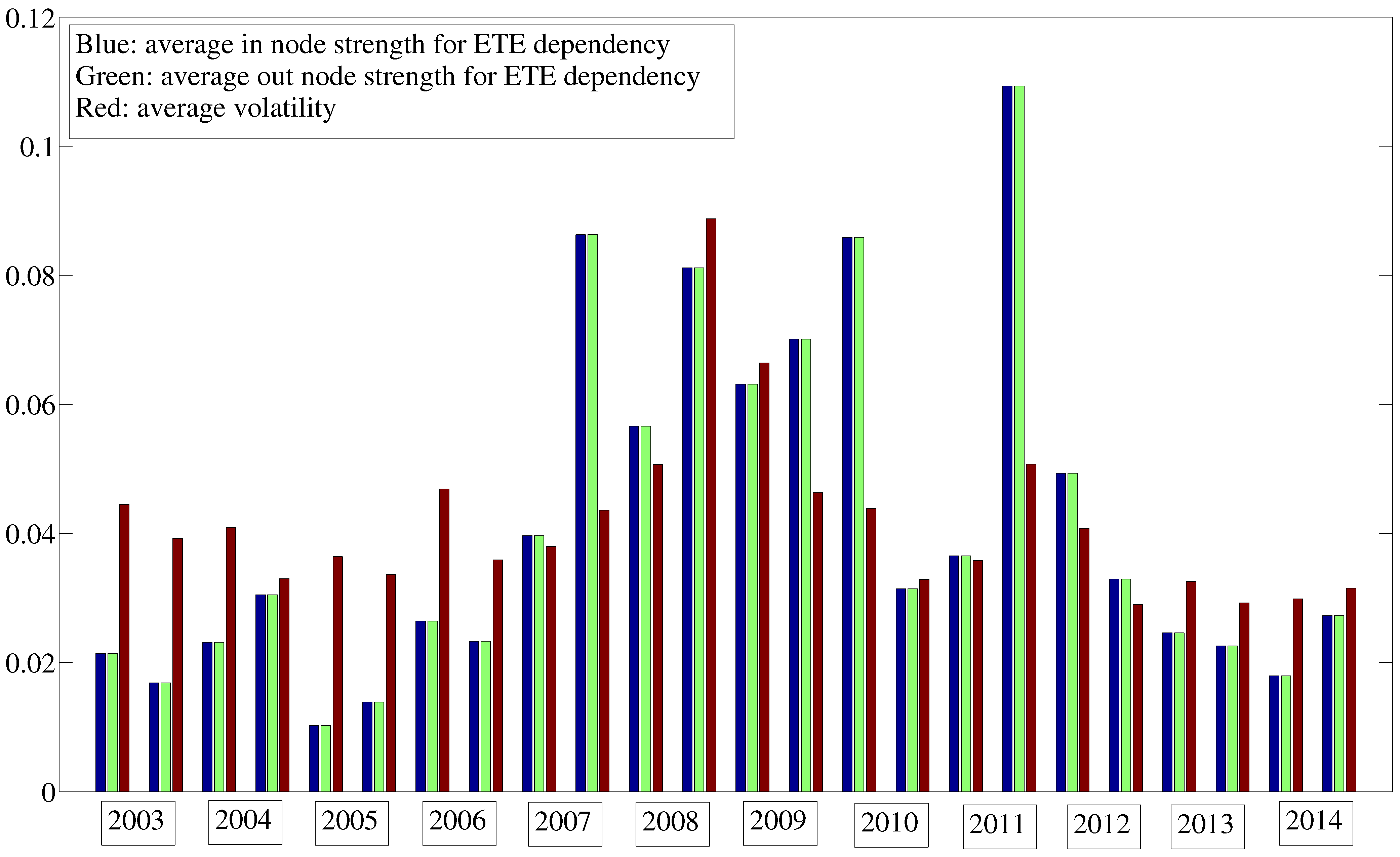
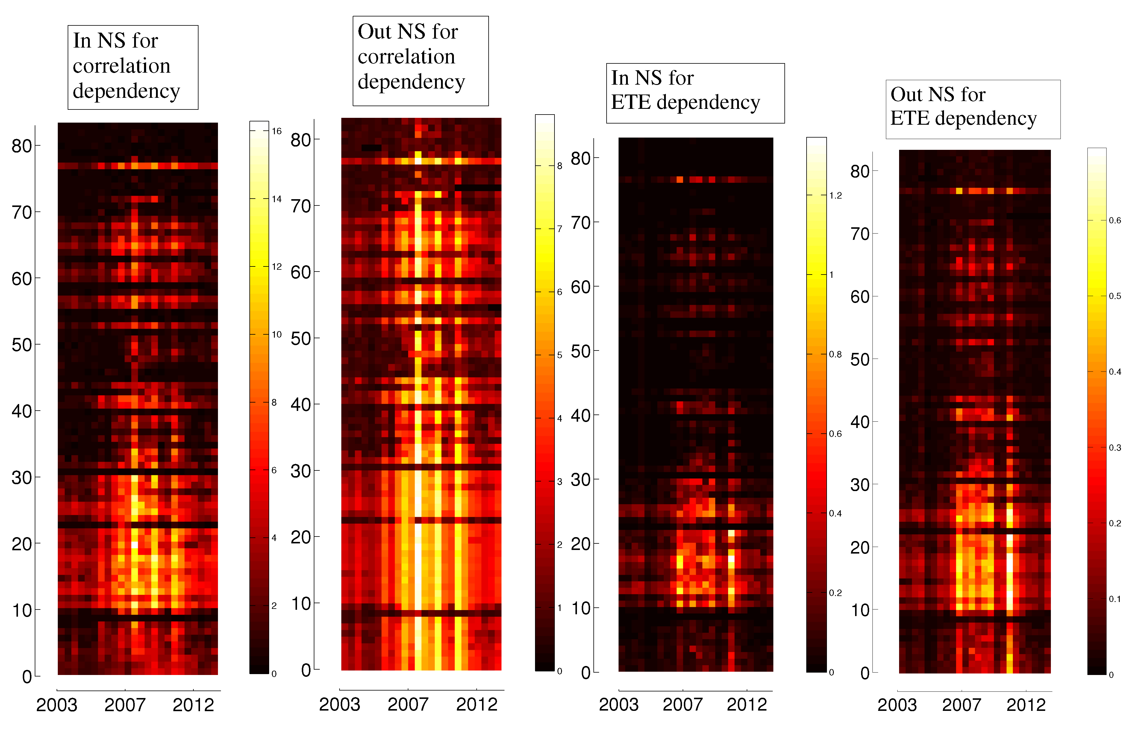
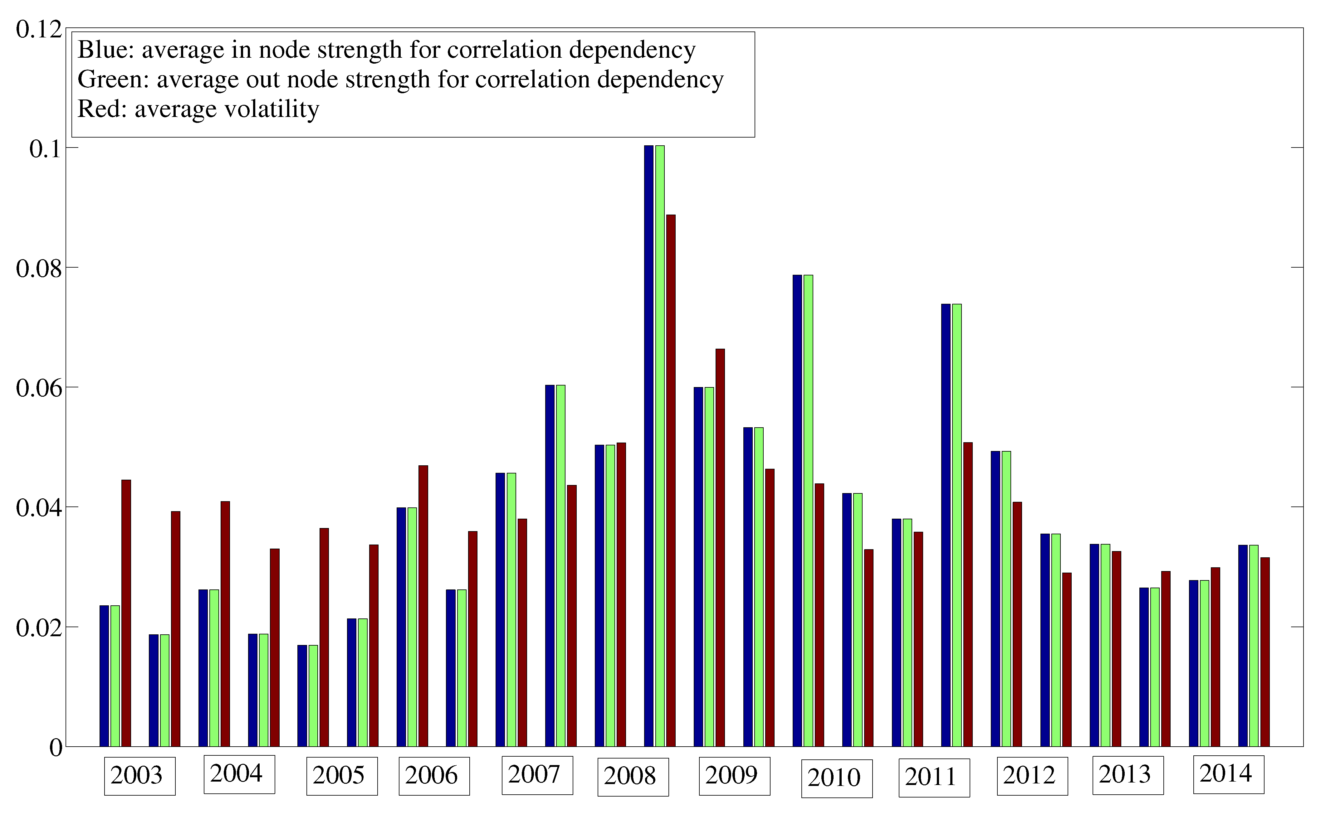
3.3. Evolution in Time

Returning to the issue of stationarity, we now make an analysis of the Pearson correlation and of the Lagged Transfer Entropy considering each year of data separately. Figure 7 shows the correlation matrices for each year, from 2003 to 2014. Although the average correlation rises in years of crisis, like 2008 and 2011, one can see that there is a conservation of the structure of the correlations between indices. Figure 8 shows the logarithmic values of a frequency distribution for each of the correlation matrices. The structure does change for years of crisis, but remains relatively intact throughout the years.
Figure 7. Correlation matrices for each of the years of data for Sector 1 (original × original variables). Brighter colors denote higher correlation, and darker colors denote lower correlations.
Jrfm 08 00227 g007
Figure 8. Logarithmic values of frequency distributions of the correlation matrices for each of the years of data for Sector 1 (original × original variables).
Jrfm 08 00227 g008
The same is shown for the Lagged Transfer Entropy (Sector 2, from lagged to original indices). Figure 9 shows the Lagged Transfer Entropy matrices for each year, from 2003 to 2014. Again, there is a conservation of the structure of the relations between indices. Figure 10 shows the logarithmic values of a frequency distribution for each of the Lagged Transfer Entropy matrices, showing that the structure does change for years of crisis, but remains relatively intact throughout the years.
Figure 9. Correlation matrices for each of the years of data for Sector 1 (original × original variables). Brighter colors denote higher correlation, and darker colors denote lower correlations.
Jrfm 08 00227 g009
Figure 10. Logarithmic values of frequency distributions of the correlation matrices for each of the years of data for Sector 1 (original × original variables).
Jrfm 08 00227 g010
So, although there is change in the data in time, the change does not affect significantly the values obtained for correlation and Transfer Entropy, particularly in terms of the structures of networks based on them. In Section 7, further discussion is made on the correlation and Transfer Entropy dependencies. Since the main aim of this article is to study the networks of indices based on measures that use correlation and Lagged Transfer Entropy, this similarity of structures in time lead us to believe that there is no significant change in the network structure derived using the whole set of data and networks based on particular subsets of data. Some confirmation of this claim may be found in [35].

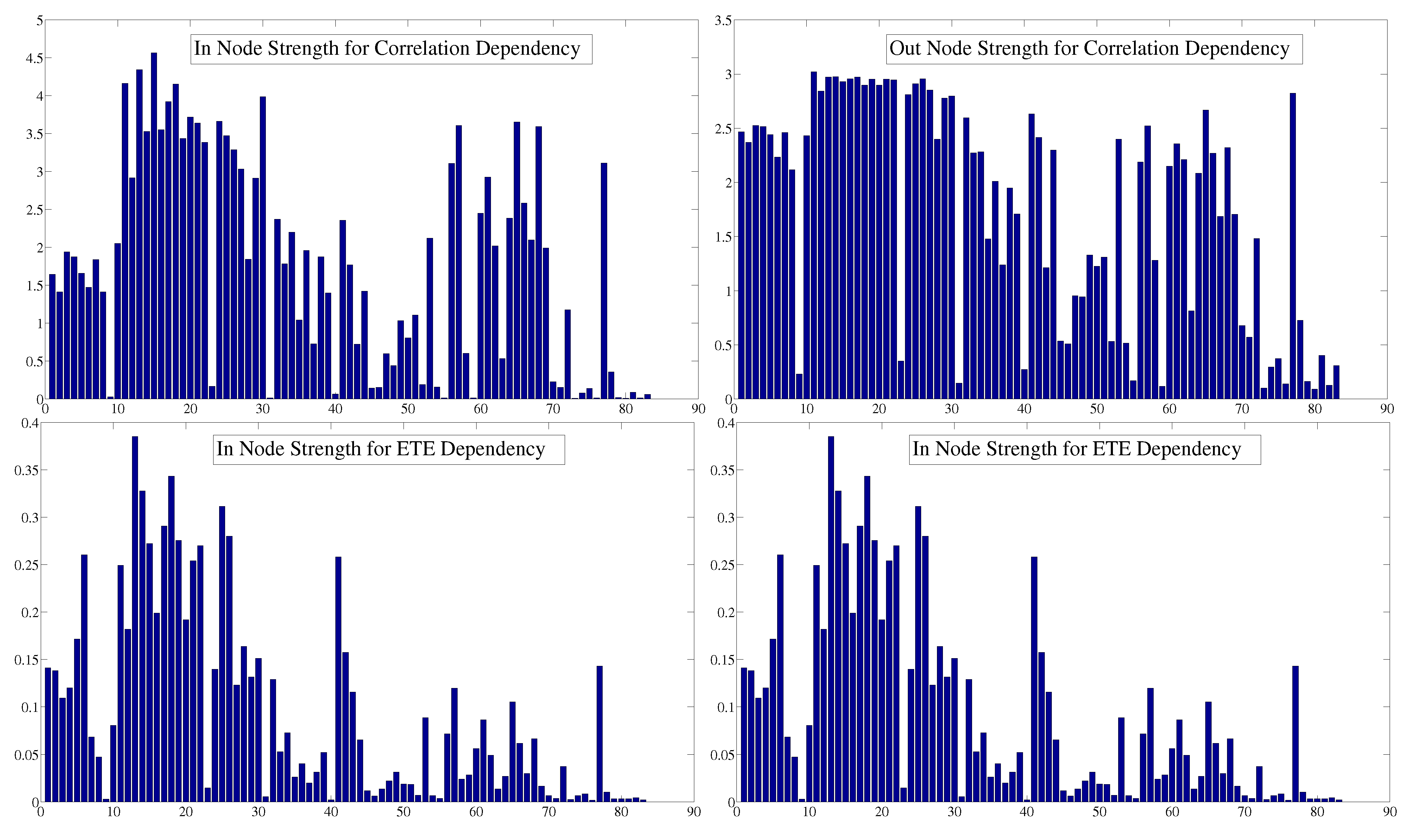
4. Dependency Networks and Node Influence

To further investigate the possibility that information flow from the previous day can anticipate correlations, we will construct a dependency or influence network [5]-a recently introduced approach to compute and investigate the mutual dependencies between network nodes from the matrices of node-node correlations. The basis of this method is to investigate the partial correlations between a given set of nodes of the network. This section describes the concept of partial correlation, influence, and dependency networks using our set of data as an example.
To construct the dependency network, we begin by calculating the partial correlations for each node from the full correlation matrix. The first order partial correlation coefficient is a statistical measure indicating how a third variable affects the correlation between two other variables [5,21]. The partial correlation between variable i and k with respect to a third variable j, P C ( i , k | j ) , is:
P C ( i , k | j ) = C ( i , k ) - C ( i , j ) C ( k , j ) ( 1 - C 2 ( i , j ) ) ( 1 - C 2 ( k , j ) )
where C ( i , j ) , C ( i , k ) and C ( j , k ) are the correlations defined in Equation (2).
The relative effect of variable j on the correlation C ( i , k ) is given by:
d ( i , k | j ) C ( i , k ) - P C ( i , k | j )
This transformation avoids the trivial case where variable j appears to strongly affect the correlation C ( i , k ) , mainly because C ( i , j ) , C ( i , k ) and C ( j , k ) have small values. We note that this quantity can be viewed either as the correlation dependency of C ( i , k ) on variable j or as the correlation influence of variable j on the correlation C ( i , k ) . Next, we define the total influence of variable j on variable i, or the dependency D ( i , j ) of variable i on variable j to be
D ( i , j ) = 1 N - 1 k j N - 1 d ( i , k | j )
The dependencies of all variables define a dependency matrix D whose i , j element is the dependency of variable i on variable j. It is important to note that while the correlation matrix C is a symmetric matrix, the dependency matrix D is not, since the influence of variable j on variable i is in general not equal to the influence of variable i on variable j.
We note that it is possible to extend the notion of partial correlations and to remove the effect of all other mediating variables. For example, the second-order partial correlation is,
P C ( i , k | j 1 , j 2 ) = P C ( i , k | j 1 ) - P C ( i , j 2 | j 1 ) P C ( k , j 2 | j 1 ) ( 1 - P C 2 ( i , j 2 | j 1 ) ) ( 1 - P C 2 ( k , j 2 | j 1 ) )
where P C ( i , k | j 1 ) , P C ( i , j 2 | j 1 ) , and P C ( k , j 2 | j 1 ) are first order partial correlations. The dependency or influence network that we describe in this work, however, is meant to reflect the influence of a particular node, j, on the interaction of node i with all other nodes. This is accomplished via removing the influence of j on the correlation between i and k, and then summing over all remaining k’s. Heuristically, the dependency matrix can be thought of as a measure of how much of the correlation between i and the rest of the nodes "flows through" j–this is distinct from the higher order partial correlation, which simply describes the direct correlation between j and k having removed all mediators, and we therefore use the first-order partial correlation to construct the dependency matrix.
In Figure 11, we plot the heat map of the dependency matrix of the full data, from 2003 to 2014, with lighter colors denoting higher values of dependency. The range of values for the dependendy matrix (based on the correlations between the original × original variables) is from 0 to 0.1454 , and the range for the lagged dependency matrix (based on the correlations between the lagged × original variables) is from - 0.0041 to 0.0891 .
Figure 11. Heat maps of the dependency matrices built on correlation for original × original indices and for lagged original indices, respectively.
Jrfm 08 00227 g011
Here we see a duplication of the structure of Figure 5 (right) and Figure 2(left), the same-day correlation matrix and the lagged ETE matrix. We also find internal structures in each quadrant. For quadrant 1 (bottom left quadrant), of original to original dependency, one finds regions of high dependency, mainly based on geographical and/or time zone differences. There is a cluster of American indices (both South and North), connected with the North American one. The indices of Central America and the Caribbeans, which are placed after Africa, are very weakly connected among themselves and to any other index. One can also see a cluster of Western European indices, with the weaker participation of Eastern European ones. There is also a weakly interacting cluster of Arab countries, and a stronger connected network of Asian Pacific indices, together with two Oceanic indices. Dependencies exist between continents as well, as can be seen by the off-diagonal brighter colors. There is also some dependency between two indices from Africa, those of South Africa and Ghana, with other indices. Looking at quadrant 4, top left one, which contains the dependencies between lagged and original indices, one can also see some dependency relations, mainly from lagged American and European indices to the next day indices of Asia Pacific and Oceania. Also of note is that, although the dependency matrix is not in principle symmetric, it does present a significant degree of symmetry among indices.
We now propose another tool with which to investigate the relations between indices: the partial transfer entropy. Recall that the transfer entropy defined above is a measure of the reduced uncertainty in the future of the destination variable Y due to knowledge of past of the source variable X. This relation can be expressed concisely in terms of conditional Shannon entropies:
T E Y X = H ( Y ( t ) | Y ( t - 1 : t - d ) ) - H ( Y ( t ) | Y ( t - 1 : t - d ) , X ( t - 1 : t - d )
where Y ( t - 1 : t - d ) represents the length-d past of the destination Y, and X ( t - 1 : t - d ) the length-d past of the source X.
We can construct a dependency matrix for the effective transfer entropy by applying the partial correlation procedure to the effective transfer entropy,
P C ( i , k | j ) = E T E ( i , k ) - E T E ( i , j ) E T E ( k , j ) ( 1 - E T E 2 ( i , j ) ) ( 1 - E T E 2 ( k , j ) )
We do so for the ETE from lagged to original indices, where the resulting matrix is represented in Figure 12 (right), and compare the result with the same day correlation dependency matrix in Figure 12 (left). Again, we see a similar structure between the dependency matrix obtained from the correlations between original variables with themselves (Sector 1 of the enlarged correlation dependency matrix) and the dependency matrix obtained from the ETEs from lagged to original indices (Sector 2 of the enlarged ETE dependency matrix). The range of values for the dependency matrix (based on the ETEs from original to original variables) is from - 0.0002 to 0.0032 , and the range for the lagged dependency matrix (based on the ETEs from lagged to original variables) is from - 0.0002 to 0.1417 . In Appendix D, we compare the effectiveness of the partial lagged ETE dependency matrix and the higher order partial lagged ETE (where the effect all mediating variables are removed) in anticipating the largest indices with the highest correlation country by country.
Figure 12. Heat maps of the dependency matrices built on ETE from original to original indices and from lagged to original indices, respectively.
Jrfm 08 00227 g012
The ETE dependency network reproduces the overall clustering structure observed in the correlation, ETE, and correlation dependency matrices, but also reveals clusters of indices within these subgroups which seem to be the strongest influencers.

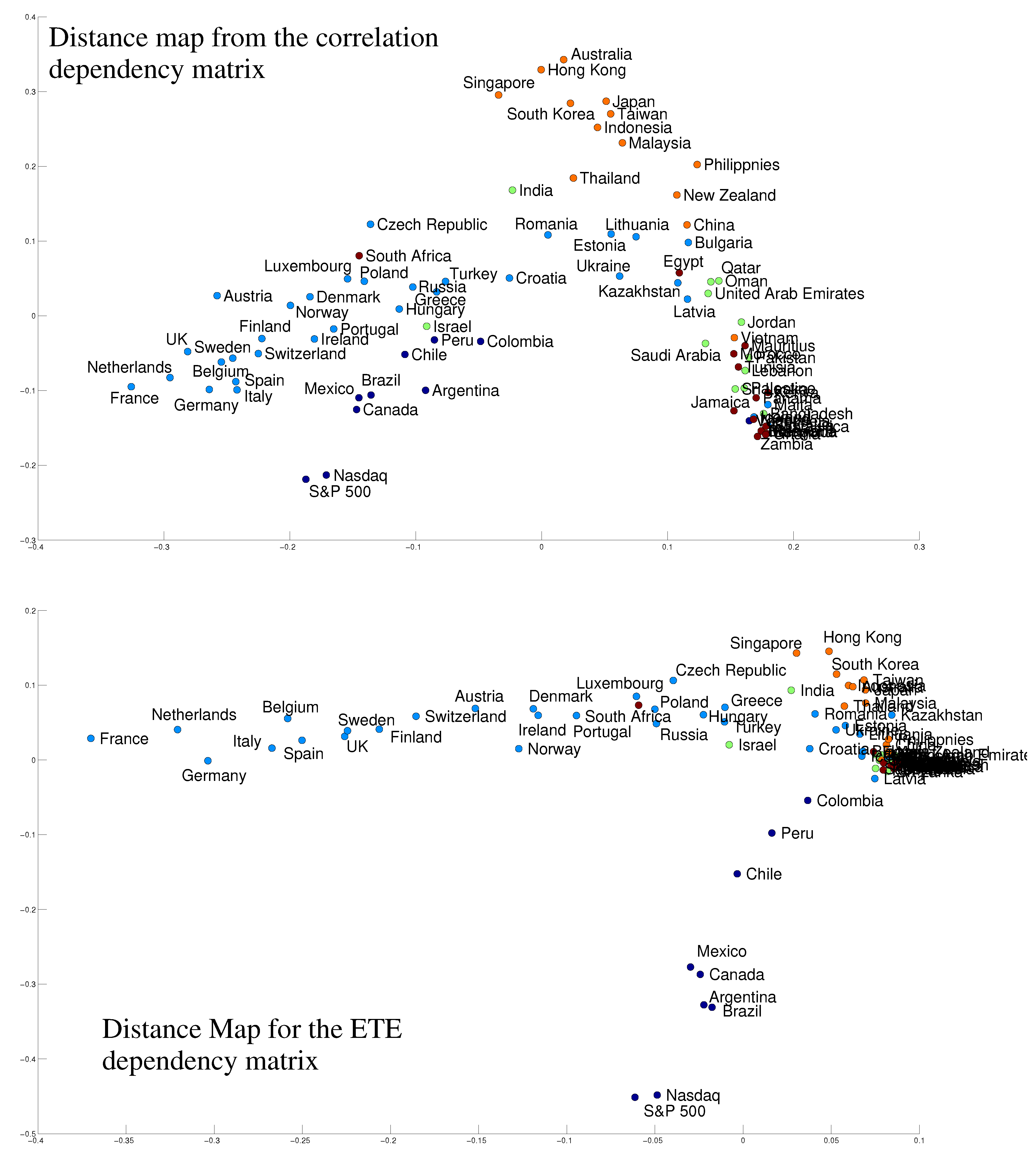
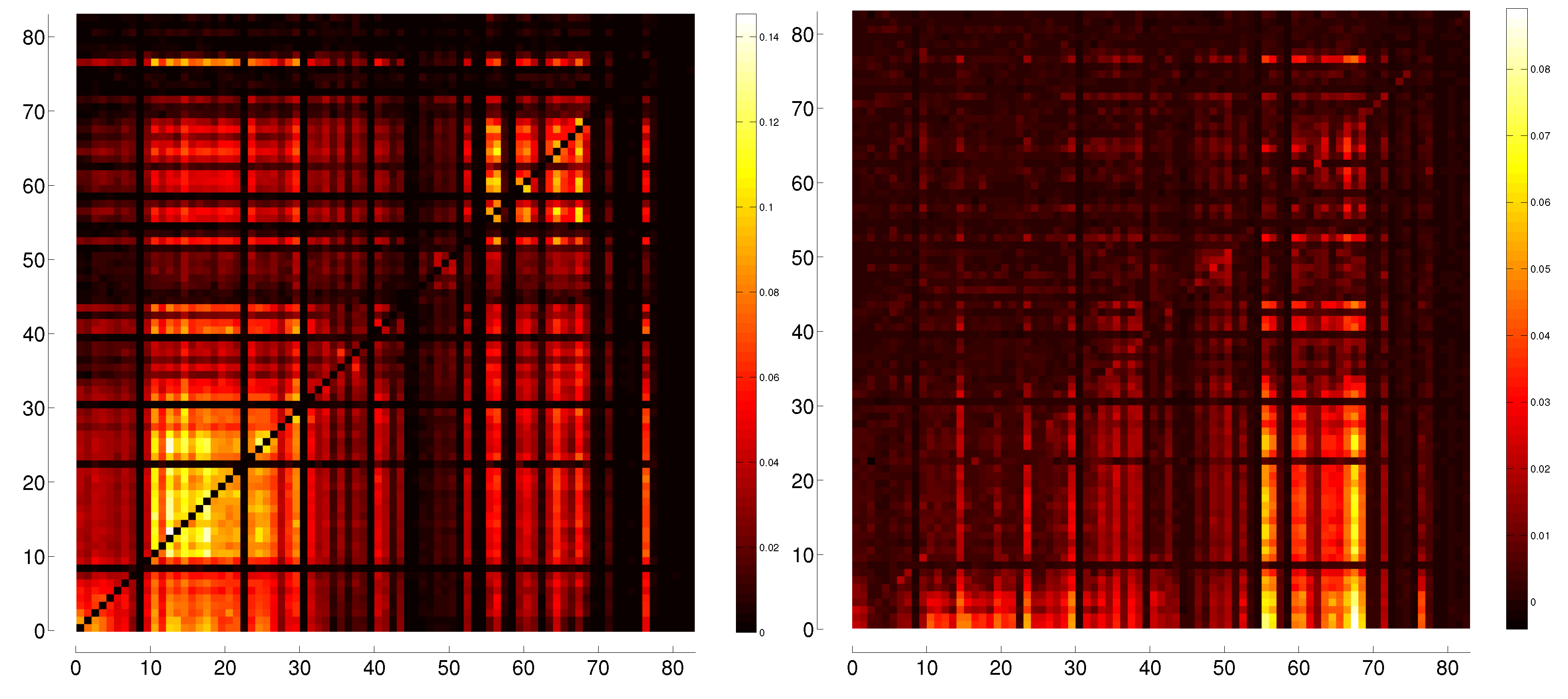
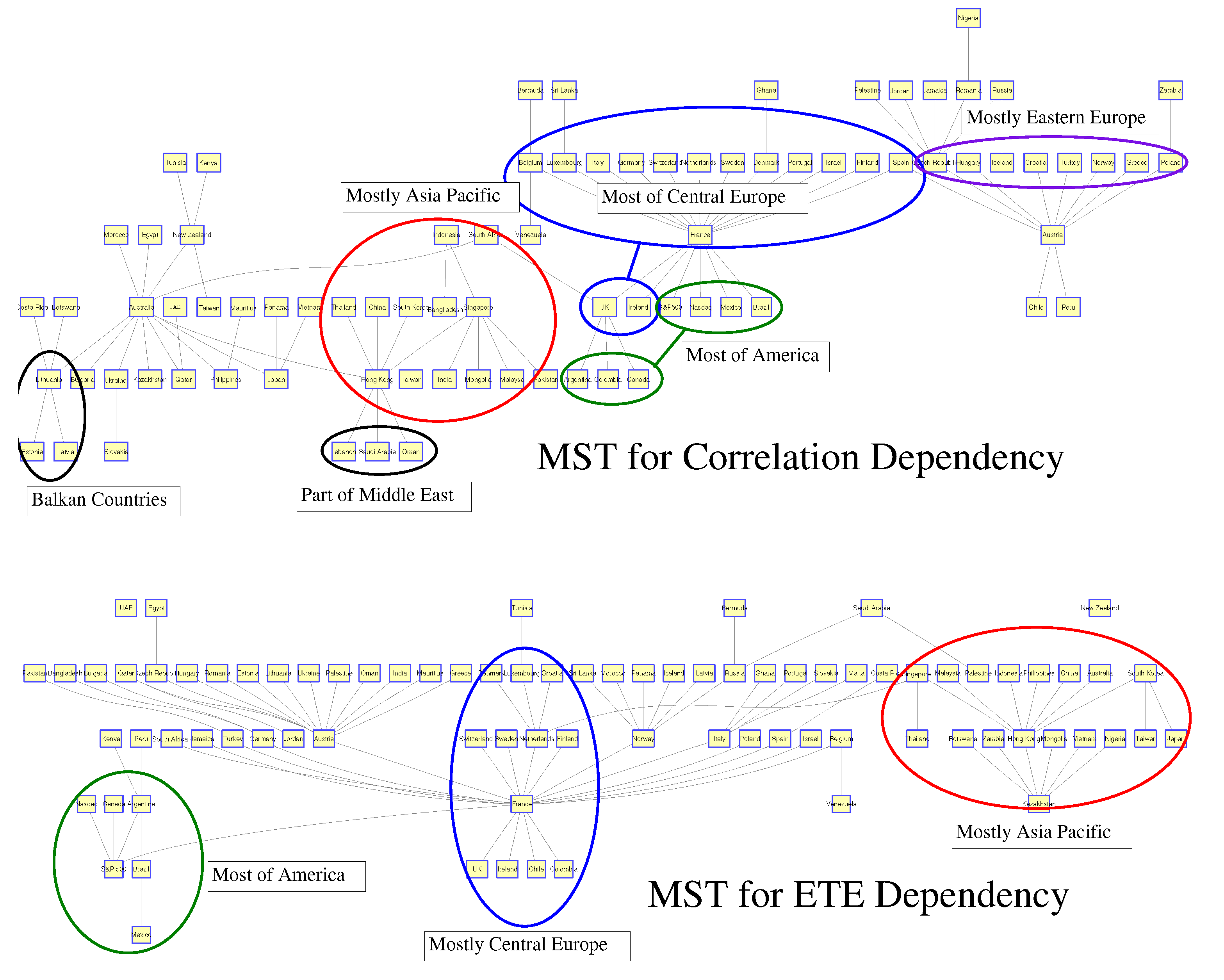
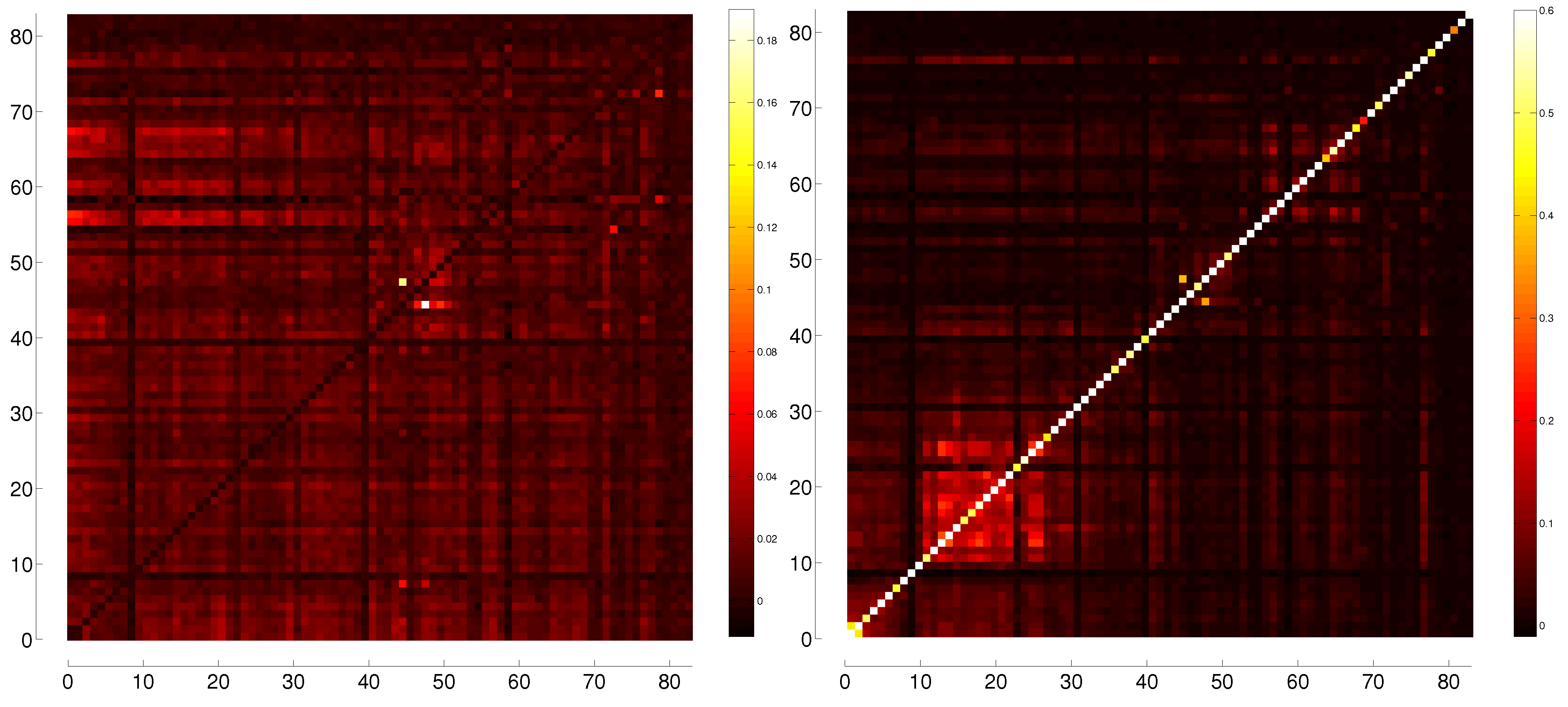
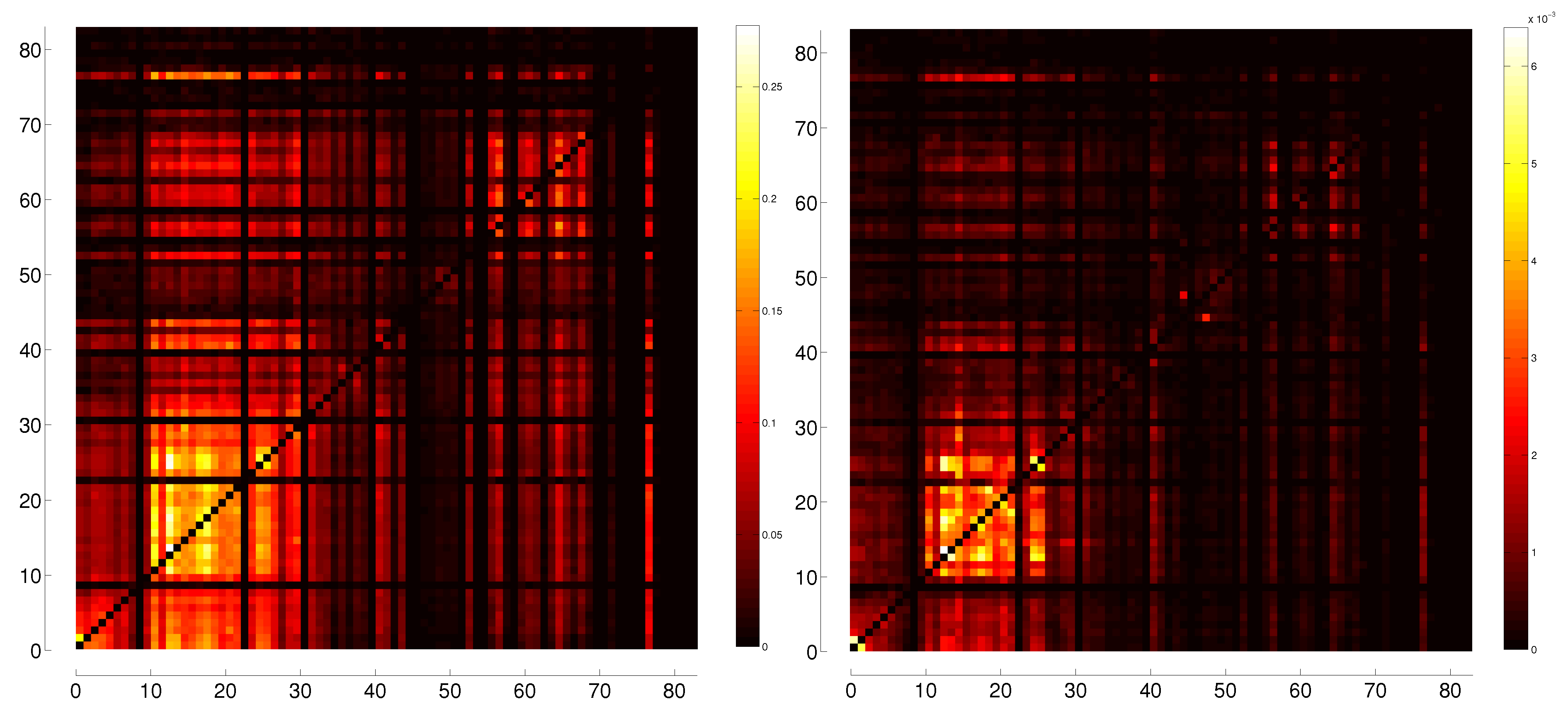
5. Representation of Correlation and Effective Transfer Entropy Dependency Networks

From the market indices we are considering, we produce two different types of networks, where the edges between nodes are either the correlation dependency between original indices or the ETE dependency from lagged indices to the original ones. These are weighted networks, since the edges between nodes are labeled by the strength of the relations between them. They are both directed networks, since the dependency matrices calculated with correlation or ETE are not symmetric.
To represent these networks, we use the technique of Classical Multidimensional Scaling [36], which assigns coordinates to each node in an m dimensional abstract space where the distances between nodes are smaller when they are strongly connected and where their distance is larger when they are poorly connected. In order to do this, we first need an appropriate measure for distance. The most common such measure in applications to financial markets is given by Mantegna [37]:
d i j = 2 1 - c i j
where, in our case, c i j is either the correlation dependency or the ETE dependency from node i to node j.
The Classical Multidimensional Scaling algorithm is based on minimizing the stress function
S = i = 1 n j > i n δ i j - d ¯ i j 2 i = 1 n j > i n d i j 2 1 / 2 , d ¯ i j = a = 1 m x i a - x j a 2 1 / 2
where δ i j is 1 for i = j and zero otherwise, n is the number of rows of the correlation matrix, and d ¯ i j is an m-dimensional Euclidean distance (which may be another type of distance for other types of multidimensional scaling). The outputs of this optimization problem are the coordinates x i a of each of the nodes, where i = 1 , , n is the number of nodes and a = 1 , , m is the number of dimensions in an m-dimensional space. The true distances are only perfectly representable in m = n dimensions, but it is possible for a network to be well represented in smaller dimensions. In our case we shall consider m = 2 , for a 2-dimensional visualization of the network, being it a compromise between fidelity to the original distances and the ease of representing the networks in a two dimensional medium.
Here we face a common problem in representing the two networks: both measures are asymmetric, whereas a distance measure must be symmetric. So, we must adopt a procedure for symmetrizing both matrices. The first procedure we follow is to normalize the correlation dependency and the ETE dependency matrices by dividing all their elements by their respective largest values. We then calculate a “distance” matrix based on each measure, and then set to zero the elements of the main diagonal of the resulting matrix. We then symmetrize the resulting matrix by setting d i j = d j i if d i j > d j i and d j i = d i j , otherwise, what means that we always consider the smallest between d i j and d j i to be the distance between i and j.
The resulting distance matrix is then used, applying Equation (16), in order to calculate a set of coordinates for each stock as a node in a space where distances are similar to the ones given by the symmetrized distance matrix. Since both dependency matrices are highly symmetric, this symmetrization procedure does not vary much if, as an examples, we use the largest “distance” instead of the smallest one, or the average of both.
The graphs resulting from this procedure are represented by Figure 13, Figure 13 (top) representing the network based on correlation dependency and Figure 13 (bottom) representing the network based on ETE dependency. The connections (edges) between nodes have not been represented, for clarity of vision. This is the way that the algorithm deals with the reduction to a two dimensional, imperfect map.
Note in both graphs that the indices that are very weakly connected to others have been placed in a bundle at a corner of the pictures. Looking now at the nodes that are placed more sparsely, one can readily see that stock markets belonging to countries that are closer together geographically, or that operate in similar time zones, have their indices represented closer together [4,38].
Another way to filter the information in the dependency matrices is a Minimum Spanning Tree (MST), which is a network of nodes that are all connected by at least one edge so that the sum of the edges is minimum, and which present no loops. This kind of tree is particularly useful for representing complex networks, filtering the information about the correlations between all nodes and presenting it in a planar graph. Because of this simplicity, minimum spanning trees have been widely used to represent a large number of important financial structures, most important for this article, of world financial markets [39,40,41,42,43,44].
Figure 14 represents the minimum spanning trees for the correlation and ETE dependencies, respectively, which were built using the distance matrices obtained previously. When looking at MSTs, one must have in mind that, since all nodes are connect to at least another node, many nodes that have very low correlation dependency or ETE dependency (meaning large distances) appear connected almost at random. This can be filtered by establishing thresholds, as an example [45], but we have not done so here.
For correlation dependency, the MST shows one cluster with mainly Central European indices, centered around France. The centrality of the French index is a result that is consistently obtained when building MSTs for international stock market indices (as in the bibliography provided). The indices of North and South America are here connected with the European indices and indirectly connected among themselves. There is a second cluster, mainly of Asia Pacific indices, and connected, and three Middle Eastern indices connected through Hong Kong. Eastern European indices appear, indirectly connected through Australia, and three Balkan indices also appear connected. For ETE dependency, the Central European and the American indices are separated into two distinct clusters, and a cluster consisting of most Asia Pacific indices. There are many other indices that have low dependency values and that seem to be almost randomly connected. Here as well France has a very central role. Again we note, through the MSTs, the clustering of indices according to geography or time zone.
Figure 13. Distance maps of the correlation and ETE dependency matrices.
Jrfm 08 00227 g013
Figure 14. Minimum Spanning Trees (MSTs) of the correlation and ETE dependency matrices.
Jrfm 08 00227 g014

6. Centrality

In financial networks, it is essential to understand which nodes are more influential or central. For weighted networks such as the ones we are considering here, Node Strength [46] is a good measure of node centrality. Node Strength is defined as the sum of all edges a node has, weighted by the values associated with each edge. Since our networks are also directed, we must calculate Node Strength for incoming and outgoing edges: In Node Strength ( N S i n ), which is the sum of the weights of all edges that go from all nodes to a particular node, and Out Node Strength ( N S o u t ), which is the sum of the weights of a node to all other nodes,
N S i n i = j = 1 N T E i j , N S o u t j = i = 1 N T E i j
So, if an index has high In Node Strength, it is more influenced (in terms of correlation dependency) and receives more information (in terms of ETE dependency) than otherwise. Similarly, if an index has high Out Node Strength, it influences more other indices, or sends more information to them, than otherwise.
Applying both centrality measures to the two networks we are studying, we obtain a rank of nodes that are more central according to each measure, represented in Figure 15. European indices are the most central, followed by some American and Asian Pacific indices. For correlation dependency, the In and Out Node Strengths are dissimilar, with the Out NS being more uniform. For the ETE dependency, both In and Out Node Strengths are very similar.
Figure 15. Node Strengths for Correlation ETE dependency.
Jrfm 08 00227 g015
The In Node Strength is a measure of the system-wide influence that a particular node has, while the Out Node Strength is a measure of how strongly influenced a node is by the system as a whole. Table 1 and Table 2 show, respectfully, the top ten most central indices according to In and Out Node Strengths, for correlation and ETE dependencies. The rule of the European indices is again apparent for ETE dependency. For both dependencies, and for In and Out Node Strengths, there is a prevalence of European indices. For correlation dependency, Austria is a receiver but not a major sender of dependency, and Germany is primarily a sender of dependency; the UK and France are both receivers and senders of dependency. The US indices appear much later in the scale of In and Out Node Strengths, with the S&P 500 in position 45, and the Nasdaq in position 47 in terms of In Node Strength for correlation dependency and with the S&P 500 in position 26, and the Nasdaq in position 33 in terms of Out Node Strength for correlation dependency, showing those indices are more influential, rather than influenced by other indices.
For ETE dependency, we have France, the Netherlands, Germany and Italy as both the major receivers and senders of information, what places them in an important place in the key stock markets in the world. The US indices again appear much later in the scale of In and Out Node Strengths, with the S&P 500 in position 22, and the Nasdaq in position 24 in terms of In Node Strength for ETE dependency and with the S&P 500 in position 21, and the Nasdaq in position 26 in terms of Out Node Strength for ETE dependency, showing those indices are more influential than influenced by other indices. We also note that the strongest sources of information are also the strongest receivers–something that is not true in the case of correlation dependency.
Why the US indices seem to play such a minor role in our results is something to be discussed. First of all, the European indices are many in comparison to the American indices, and they form a tight cluster, what favours all centrality measures, even the weighted ones. Second, if one would plot a distance map of stocks belonging to the Central European stock markets (something that has been done by one of the authors in a separate, yet unpublished work), one would see that European stocks form a cluster where there is no separation according to country, and that American stocks separate mainly according to country. So, the indices of Central European countries are the results of separating stocks that are clustered together, and they are merely aspects of the same stock market. Figure 15 shows, though, that the influence of the American indices in terms of correlation (Ou NS) is more similar in strength to the influence of Central European indices.
Table 1. Top ten indices according to In and Out Node Strengths based on correlation dependency.
Correlation Dependency
IndexIn NSIndexOut NS
Austria4.57UK3.02
France4.35Germany2.98
UK4.16France2.97
Netherlands4.15Belgium2.97
Czech Republic3.99Switzerland2.96
Belgium3.93Spain2.96
Denmark3.72Sweden2.95
Luxembourg3.66Norway2.95
Singapore3.66Finland2.95
Norway3.63Austria2.93
Table 2. Top ten indices according to In and Out Node Strengths based on ETE dependency.
ETE Dependency
IndexIn NSIndexOut NS
France0.39France0.32
Netherlands0.34Netherlands0.29
Germany0.33Germany0.28
Italy0.31Italy0.28
Belgium0.29Spain0.26
Spain0.28Belgium0.25
Sweden0.28Sweden0.25
Austria0.27Finland0.24
Finland0.27UK0.23
Argentina0.26Austria0.22
In order to go deeper in the understanding of what Table 1 and Table 2 mean, we must remember what dependency means for both correlation and ETE. In the first case, dependency means how one index affects the correlation of another index with all the others, or how “alike” its time series is in comparison with others. The UK and Germany then appear as major influencers in the closed knitted network of Central European indices, while Austria and France appear as the ones who are most led to be “like” other indices. In all previous computations of simple correlations between stock market indices, France always appears as the most correlated stock market while Austria is not so well correlated. Since the Central European indices are actually part of a single cluster of stocks, we might be seeing results distorted by this fact. Looking at Figure 15, the Out Node Strengths of most Central European indices are similar, and so any classification of indices is disputable.
Now, the dependency for ETE means the amount that an index influences the way the knowledge of the time series of other indices may help to lessen uncertainties in the time series of all the others. This seems to be very symmetric, and the effect of Central Europe being a cluster of stocks may also influence results. A deeper study of the European stock markets and of how an integrated market works would be a good topic for future research.

7. Dynamics

Our data span 11 years of the evolution of most of the world’s stock market indices, through times of both low and high volatilities. By plotting heat maps of correlation, effective Transfer Entropy, correlation dependency, and ETE dependency, not shown here, we observe how these measures change in time, particularly in times of high volatility.
In order to study the dynamics of the correlation and ETE dependency networks, we split the original data into semesters, comprising roughly 125 days of operation each, and calculated their correlation and ETE dependency matrices. We use binning of width 0.5 here, and not 0.02 like in previous calculations, because there are fewer data now, and a binning too thin would lead to many zero joint probabilities. Then, we calculated the mean of each matrix and compared it to the average volatility of the stock markets in each semester calculated as the mean of the absolute values of all indices in that semester. For some semesters, we had some problems in calculating the correlations involving the indices from Bangladesh, Gahna, and Kenya, due to low liquidity of those indices. Those problems were solved by fixing the correlation matrix of these indices to others as zero, whenever that correlation was impossible to calculate. This problem did not happen to ETE.
Figure 16 and Figure 17 show the results, where the bars were normalized so that the sum of the columns for each measure were set to 1. We can see that the average correlation dependency follows approximately the average volatility of the world market, with an increased value after the crisis of 2008 even though volatility fell after that crisis. Now, the average ETE dependency remained smaller than the average volatility before the crisis of 2008, and it remained high after the crisis, and in particular during the crisis of 2011.
Figure 16. Average correlation dependency × average volatility.
Jrfm 08 00227 g016
Figure 17. Average ETE dependency × average volatility.
Jrfm 08 00227 g017
Figure 18 shows the evolution of the In and Out Node Strengths of the individual indices, with brighter colors for larger values and darker colors for smaller values. For all measures, the European indices present the largest values, followed by American and Asian Pacific indices, plus South Africa. We may see that correlation and ETE dependencies are stronger during the crises of 2008 and of 2011. We may also notice that the Out Node Strengths are consistently larger than the In Node Strengths for all measures, so there is more influence or information being sent than received by the indices.
Figure 18. Evolution of in and out node strengths for correlation and ETE dependencies.
Jrfm 08 00227 g018

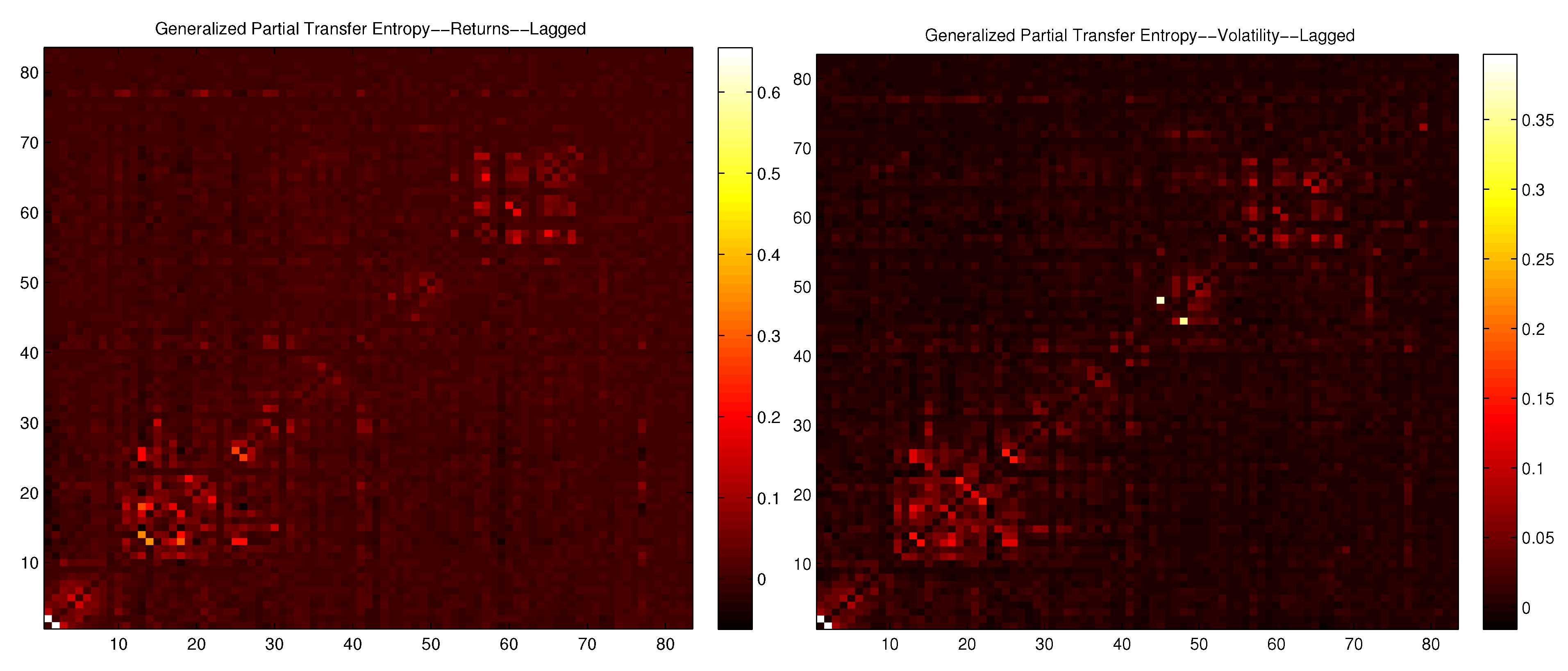
8. Dependencies for Volatility

One of the known facts in financial data is the volatility clustering [47], what means that, although financial data time series usually show low autocorrelation of log returns, the time series of absolute values or of standard deviations (both known as volatility) present a larger autocorrelation. This means that, although the time series of log returns does not present a long memory, the time series of volatility does present a longer memory, which in terms of daily log returns may span some days. So, it is expected that lagged correlation and lagged ETE and their dependency versions will magnify effects seen for their counterparts based on log returns.
Figure 19 presents the heat maps of the correlation and lagged correlation matrices for the absolute values of the log returns, and Figure 20 shows the heat maps for the ETE and LETE matrices of the absolute values of the log returns. The values for correlation go from - 0.1143 to 1, and for lagged correlation from - 0.3227 to 0.5657 . Both heat maps are represented so that the lowest value is in black and the largest value is in white. For ETE, the values go from - 0.0114 to 0.1899 , and for LETE values from - 0.0105 to 1.4328 . For the LETE heat map, the maximum was set to 0.6 (so values above this are shown as white) in order to enhance visibility.
Figure 19. Heat maps of the correlation and lagged correlation matrices for the absolute values of log returns.
Jrfm 08 00227 g019
Figure 20. Heat maps of the correlation and lagged ETE matrices for the absolute values of log returns.
Jrfm 08 00227 g020
Table Table 3 shows the minimum and maximum values of correlations and ETEs for log-returns and volatility, and also for correlation and ETE dependencies. Comparing the correlation matrices obtained for volatility (Figure 19) with the ones obtained for log-returns (Figure 2), one can see that volatilities are less prone to anticorrelation than log-returns, what can be seen from the less negative minimum values for volatilities for both original × original and lagged × original correlations. For ETE, there is not much difference between results obtained from log-returns or volatility, except for the maximum values of LETE, which is lower for volatilities.
Table 3. Minimum and maximum values of Correlations, ETEs, and dependencies, for log-returns and for volatility, for original and lagged matrices. Numbers in brackets show maximum off-diagonal values.
Mininum ValueMaximum Value
Correlation of log-returns–0.11431 (0.9485)
Correlation of volatility–0.08901 (0.9236)
Lagged Correlation of log-returns–0.32270.5657
Lagged Correlation of volatility–0.11060.4977
ETE of log-returns–0.01620.1691
ETE of volatility–0.01140.1899
LETE of log-returns0.00402.0265 (0.7386)
LETE of volatility–0.01051.4328 (0.4282)
Correlation Dependency of log-returns00.1454
Correlation Dependency of volatility00.2774
ETE Dependency of log-returns–0.00020.1417
ETE Dependency of volatility00.0064
Figure 21 shows the heat maps of the dependency matrices based on correlation and on LETE, respectively. For correlation dependency, the values go from 0 to 0.2774 , and for LETE dependency, the values go from 0 to 0.0225 . According to Table 2, the ETE maximum dependency for volatilities is slightly higher than for log-returns, but the ETE maximum dependency for log-returns is much higher than for the maximum dependency for volatilities.
Figure 21. Heat maps of the dependency matrices based on correlation and on LETE, respectively, based on the absolute values of log returns.
Jrfm 08 00227 g021
So, although we expected correlation and ETE and their dependencies were higher for volatilities, results showed that there is no substantial change in results if we use volatilities instead of log-returns. The fact that TE and ETE filter out the past influence of a variable on itself may lessen the strong effect of autocorrelation typical of volatilities.

8.1. Oil Producing Nations

We have argued that the dependency matrix approach, together with the transfer entropy, provides a useful tool for the analysis of financial networks, and which may help to uncover information that remains hidden to strictly correlation based methods. As a final example, we apply our partial lagged transfer entropy analysis to the oil producing countries appearing in our list of indices, to determine whether our information based measure is able to uncover connections in this important subsector of the world economy.
Table 4 presents a list of 10 of the worlds top oil producers–together accounting for over 65% of world oil production–and their five most significant “influencers”. The top row for each country contains the ranked list of the countries which most strongly correlate with the volatility of the oil producer, and the bottom row contains the strongest influencer ranked by lagged partial ETE. Remarkably, we find that the lagged partial ETE list’s contain more of the top oil producers among the top influencers than the simple correlations. This suggests that the lagged partial ETE is revealing a flow of information that is not reflected in the correlations between these indices. We should note that the better developed economies on our list–the US, Canada, China, Russia, Brazil, and Norway–do not display this pattern, perhaps due to having other important economic sectors whose information flows wash out the signal from other oil producers, or due to the fact that the signal is already strong enough to appear in the volatility correlation. Nevertheless, we feel that this pattern warrants further investigation.
Table 4. Top five contributors to volatility correlation and to volatility dependency for major oil producing nations. In bold are those countries that appear in the dependency but not in the correlation list.
OIL PRODUCERMost Influenced by
Russia (Volatility Correlation)NorwayCzech RepublicSouth AfricaAustriaUK
Russia (Volatility Dependence)NorwayCzech RepublicUkraineAustriaSouth Africa
Saudi Arabia (Volatility Correlation)PalestineOmanIndonesiaQatarJordan
Saudi Arabia (Volatility Dependence)PalestineIndonesiaRussiaCanadaQatar
USA (SP) (Volatility Correlation)USA(Nas)CanadaMexicoBrazilGermany
USA (SP) (Volatility Dependence)USA(Nas)CanadaMexicoGermanyBrazil
USA (Nas) (Volatility Correlation)USA(SP)CanadaMexicoBrazilGermany
USA (Nas) (Volatility Dependence)USA(SP)CanadaBrazilGermanyFrance
China (Volatility Correlation)Hong KongSingaporeTaiwanAustraliaSouth Korea
China (Volatility Dependence)Hong KongTaiwanSouth KoreaSingaporeVietnam
Canada (Volatility Correlation)USA(SP)USA(Nas)NorwayBrazilMexico
Canada (Volatility Dependence)USA(SP)USA(Nas)BrazilMexicoArgentina
UAE (Volatility Correlation)QatarOmanJordanEgyptCzech Republic
UAE (Volatility Dependence)QatarOmanPalestineJordanSaudi Arabia
Venezuela (Volatility Correlation)Costa RicaColombiaJamaicaPalestineChile
Venezuela (Volatility Dependence)ColombiaBrazilArgentinaMongoliaSaudi Arabia
Mexico (Volatility Correlation)USA(SP)USA(Nas)BrazilCanadaUK
Mexico (Volatility Dependence)BrazilUSA(SP)USA(Nas)ArgentinaNorway
Brazil (Volatility Correlation)USA(SP)MexicoUSA(Nas)CanadaNetherlands
Brazil (Volatility Dependence)MexicoArgentinaUSA(Nas)USA(SP)Canada
Norway (Volatility Correlation)UKNetherlandsSwedenFranceAustria
Norway (Volatility Dependence)DenmarkAustriaSwedenFinlandNetherlands

9. Conclusions

We’ve used the information-based measures of effective Transfer Entropy and partial effective Transfer Entropy to uncover the flow of information between 83 international market indices and their one-day lagged values. The structure of one-day lagged information flow between market indices is seen to be very similar to same-day index correlation, which suggests that information flow between markets, as modelled by effective Transfer Entropy, is an effective way of quantifying the interaction of stock market indices. Additionally, we apply the recently introduced dependency network method, based on partial correlation between variables, to develop a more fine grained view of which indices are the strongest influencers of market interaction. The methods developed and applied in this work serve as a proof-of-concept which we intend to apply, in future work, to study the precise relationship between strongly influencing nodes and the subgroup of indices to which they belong, as well as to the question of how these “information center” nodes affect network topology and the propagation of unexpected events.

Acknowledgments

AM acknowledges support from the Boston University Physics department, and DYK acknowledges support from the Boston University Physics Department and the Center for Polymer Studies at Boston University. This article was written using Jrfm 08 00227 i001, all figures were made using Matlab or PSTricks, and the calculations were made using Matlab and Excel. All data and codes used are freely available upon request on [email protected].

Author Contributions

LS and DYK conceived the project; LS, AM, and DYK performed the calculations and analysis, and wrote the article.

A. Indices and Countries they Belong to

NumberCountryIndex
1S& P 500S& P 500 Index
2NasdaqNasdaq Composite Index
3CanadaS& P/TSX Composite Index
4MexicoMexico Stock Exchange IPC Index
5BrazilIvovespa São Paulo Stock Exchange Index
6ArgentinaBuenos Aires Stock Exchange Merval Index
7ChileSantiago Stock Exchange IPSA Index
8ColombiaIndice IGBC
9VenezuelaCaracas Stock Exchange Market Index
10PeruBolsa de Valores de Lima General Sector Index
11UKFTSE 100 Index
12IrelandISEQ Overall Index
13FranceCAC 40 Index
14GermanyDAX Index
15ATXAustrian Traded Index
16SwitzerlandSwiss Market Index
17BelgiumBEL 20 Index
18NetherlandsAEX Index
19SwedenOMX Stockholm 30 Index
20KFXOMX Copenhagen 20 Index
21NorwayOBX Oslo Index
22FinlandOMX Helsinki All-Share Index
23IcelandOMX Iceland All-Share Index
24LuxembourgLuxembourg LuxX Index
25ItalyFTSE MIB
26SpainIBEX 35 Index
27PortugalPortugal PSI 20 Index
28GreeceAthens Stock Exchange General Index
29PolandWarsaw Stock Exchange WIG Index
30Czech RepublicPX Index
31SlovakiaSlovak Share Index
32HungaryBudapest Stock Exchange Index
33CroatiaCROBEX
34RomaniaBucharest Exchange Trading Index
35BulgariaBulgaria Stock Exchange Sofix Index
36EstoniaOMX Tallinn
37LatviaOMX Riga
38LithuaniaOMX Vilnius
39UkraineUkraine PFTS Index
40MaltaMalta Stock Exchange Index
41RussiaMICEX Index
42TurkeyBorsa Istambul 100
43KazakhstanKazakhstan Stock Exchange Index KASE
44IsraelTel Aviv 25 Index
45PalestinePalestine Al Quda Index
46LebanonBLOM Stock Index
47JordanASE General Index
48Saudi ArabiaTadawul All Share Index
49QatarQE Index
50United Arab EmiratesADX General Index
51OmanMSM Index
52PakistanKarachi Stock Exchange KSE100 Index
53IndiaS& P BSE Sensex Index
54Sri LankaSri Lanka Stock Market Colombo All-Share Index
55BangladeshDSE General Index
56JapanNikkei-225 Stock Average
57Hong KongHang Seng Index
58ChinaShanghai Stock Exchange Composite Index
59MongoliaMSE Top 20 Index
60TaiwanTWSE
61South KoreaKOSPI Index
62ThailandBangkok SET Index
63VietnamVietnam Stock Index
64MalaysiaFTSE Bursa Malaysia KLCI Index
65SingaporeStraits Times Index
66IndonesiaJakarta Stock Price Index
67PhilippniesPhilippine Stock Exchange PSEi Index
68AustraliaS& P/ASX 200
69New ZealandNew Zealand Exchange 50 Gross Index
70MoroccoCFG 25
71TunisiaTunis Stock Exchange TUNINDEX
72EgyptEGX 30 Index
73GhanaGSE Composite Index
74NigeriaNigerian Stock Exchange All Share Index
75KenyaNairobi Securities Exchange Ltd 20 Share Index
76BotswanaBotswana Domestic Companies Gaborone Index
77South AfricaFTSE/JSE Africa All Shares Index
78MauritiusSEMDEX Index
79ZambiaLusaka Stock Exchange All Share Index
80BermudaBermuda Stock Exchange Index
81JamaicaJamaica Stock Exchange Market Index
82Costa RicaBCT Corp Costa Rica Stock Market Index
83PanamaBolsa de Valores de Panama General Index

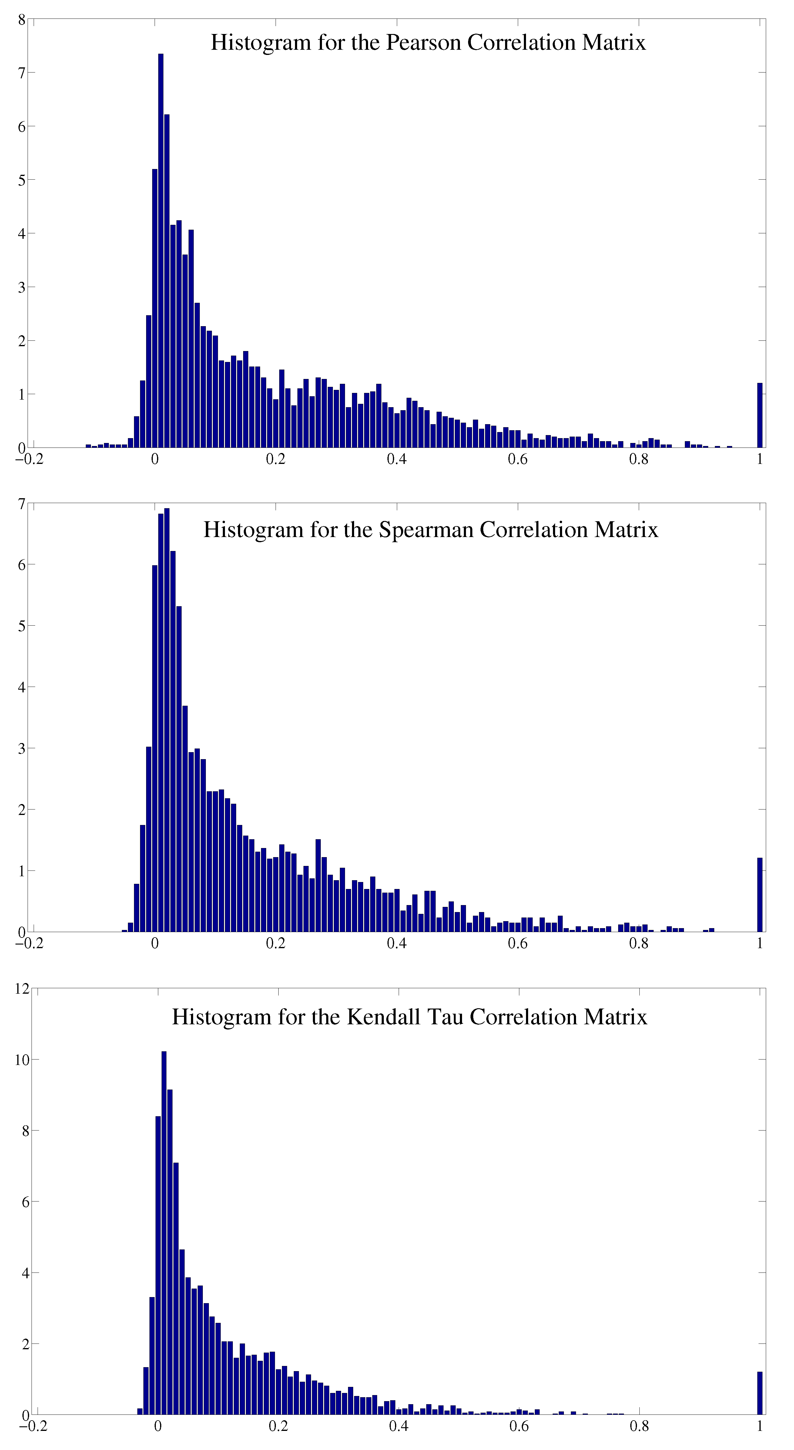
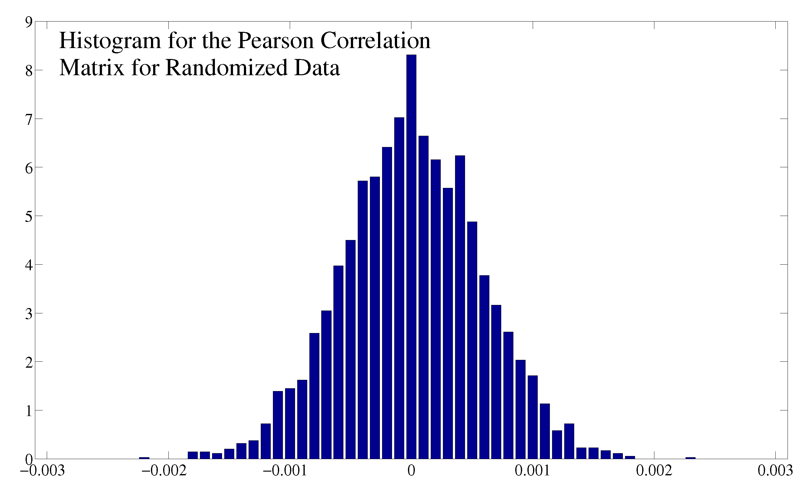
B. Comparison between Different Correlation Measures

One issue that arises from our analysis of correlation between indices is if the Pearson correlation is the appropriate measure, since it only measures linear correlations. The Spearman rank correlation and the Kendall tau rank correlation are two measures capable of detecting nonlinear correlations between variables. So, in this Appendix, we show the correlation matrices containing the correlations between all indices by using three correlation measures: the Pearson correlation, the Spearman rank correlation, and the Kendall tau rank correlation. The resulting correlation matrices are represented in Figure 22 in terms of heat maps. One may notice that there are no significant differences between them, what suggests that most correlations are captured by the Pearson linear correlation.
Figure 23 shows the histograms of the elements of the three correlation matrices, showing that there is not much difference in structure between the three. So, we have ground for using the Pearson correlation in our calculations, which is much faster to calculate and captures the same correlation structure as other correlation measures, more useful for nonlinear correlations.
Figure 24 shows the histogram for the elements of the average of the Pearson correlation matrices obtained from ten simulations with randomized data. The distribution is close to a Gaussian, and the values go from - 0.0022 to 0.0023 for off-diagonal elements, a small interval when compared with the values from - 0.1143 to 0.9485 of the Pearson correlation matrix obtained from the original data.
Figure 22. Correlation matrices using three different correlation measures: Pearson correlation, Spearman rank correlation, and Kendall tau rank correlation, respectively.
Jrfm 08 00227 g022
Figure 23. Histograms of the elements of the correlation matrices obtained from three different correlation measures: Pearson correlation, Spearman rank correlation, and Kendall tau rank correlation, respectively.
Jrfm 08 00227 g023
Figure 24. Histograms of the elements of the correlation matrix obtained as the average of ten Pearson correlation matrices of simulations with randomized data, where the diagonal terms (always equal to 1) have been removed.
Jrfm 08 00227 g024

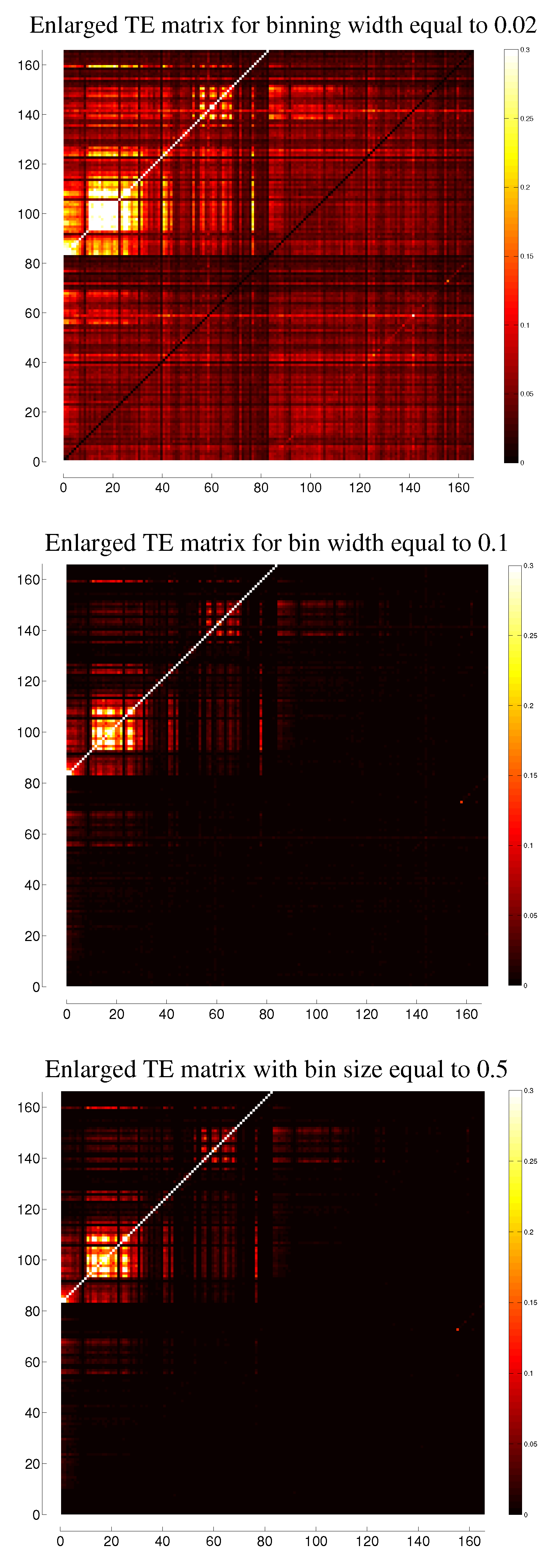
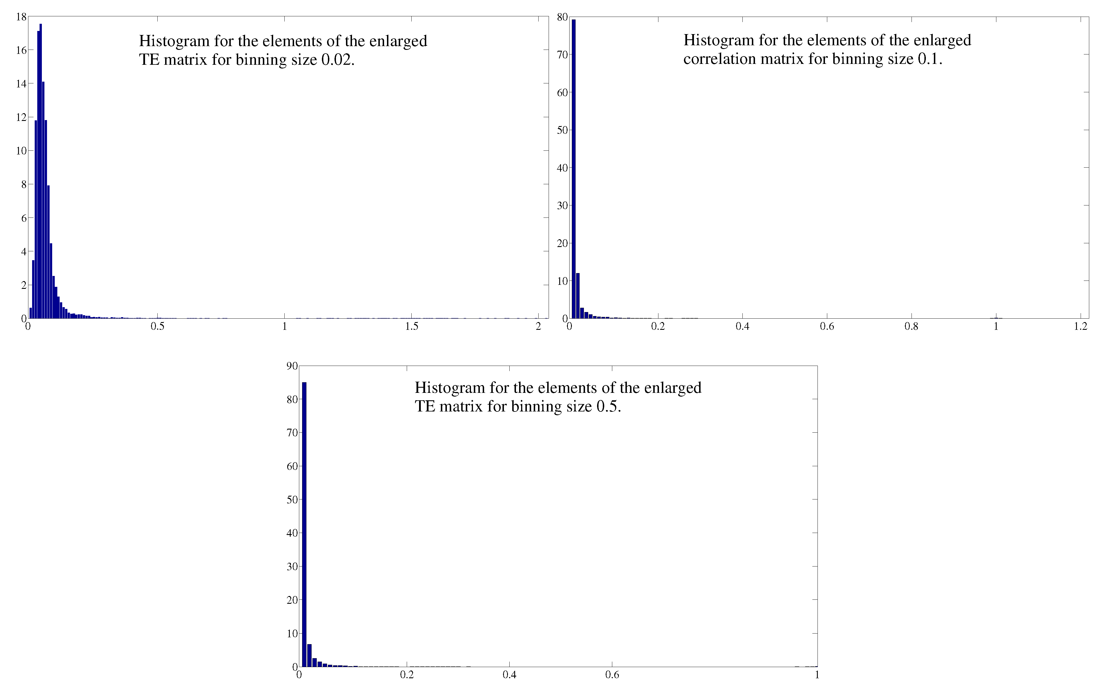
C. Comparison between Different Binnings for Transfer Entropy

The calculation of Transfer Entropy involves the discretization of the variables into bins. This binning may be varied so as to lead to a large number of bins with low values of probability for each one or larger bins with larger probabilities. Since our calculations involve the joint probabilities of three different variables, using too many bins may render each probability too close to zero, but using few bins may lead to some loss in the precision with which we compare different variables. In order to probe the differences in Transfer Entropy obtained using different binnings, in this Appendix we compare the Transfer Entropy matrices obtained with three different binnings. Our set of data contains log returns that run from - 1.0622 to 1.0697 , so that using bins with width equal to 0.02 , we have at most 108 different bins; for bins with width equal to 0.1 , we have 23 different bins; and for bins of width 0.5 , we have 5 bins. Figure 25 shows the Enlarged TE matrices obtained using these three sizes of binning, 0.02 , 0.1 , and 0.5 , respectively. The largest brightness for all three heat maps was set to 0.3 (so, every cell with TE value above 0.3 is painted white) in order to make the figures more visible.
The enlarged TE matrix for binning 0.02 has elements ranging from 0 to 2.0265 ; the enlarged TE matrix for binning 0.1 has elements ranging from 0 to 1.2054 ; and the enlarged TE matrix for binning 0.5 has elements ranging from 0 to 0.9999 . This is expected, since a smaller bin size generates a larger number of bins and thus of probabilities that are computed by TE. Although the range of values for each enlarged TE matrix is different, the heat maps show a very similar structure for each of them, what can be reinforced by comparing the histograms of the TE matrices’ elements shown in Figure 26.
Figure 25. Enlarged TE matrices using three different binning sizes: 0.02, 0.1, and 0.5, respectively.
Jrfm 08 00227 g025
Figure 26. Histograms of the elements of the enlarged TE matrices obtained using three different binning sizes: 0.02, 0.1, and 0.5, respectively.
Jrfm 08 00227 g026

D. Partial Lagged ETE and Generalized Partial Lagged ETE

We now compare the effectiveness of the generalized, higher order, partial lagged ETE (ie, with the effects of all mediating variables removed) to the partial lagged ETE dependency matrix which we have introduced, in anticipating the same day correlations of the returns and volatilities of the indices in our data set.
Figure 27 displays the generalized partial lagged ETE matrix for both the log-returns (left) and the volatilities (right), that is, each entry is the direct lagged-to-original ETE between the y-index and the x-index with the effects of all others removed. For example, the 11th entry in the 1st column of the volatility heat map corresponds to the flow of Shannon information from the previous day UK FTSE 100 index to the next day US S&P 500 index. As is readily seen, this matrix lacks much of the robust structure observed in the correlation matrices and in the dependency matrices. However, there is still a clear similarity in overall clustering and index importance. Additionally, we ranked the top 10 entries in each column for the correlation, generalized partial correlation, and lagged ETE dependency matrices, and compared the lists to determine which of the two latter measures best approximated the “top 10” in the correlation list. We found that in the large majority of cases the dependency matrix approach more closely reflected the correlations.
Figure 27. Generalized partial Tranfer Entropy of the log-returns (left) and of the volatilities (right), from lagged to original variables.
Jrfm 08 00227 g027

Conflicts of Interest

The authors declare no conflict of interest.

References

  1. F. Allen, and D. Gale. “Financial contagion.” J. Polit. Econ. 108 (2000): 1–33. [Google Scholar] [CrossRef]
  2. L. Sandoval Jr. “Structure of a Global Network of Financial Companies based on Transfer Entropy.” Entropy 16 (2014): 4443–4482. [Google Scholar] [CrossRef]
  3. L. Sandoval Jr., and I.D.P. Franca. “Correlation of financial markets in times of crisis.” Phys. A 391 (2012): 187–208. [Google Scholar]
  4. L. Sandoval Jr. “To lag or not to lag? How to compare indices of stock markets that operate at different times.” Phys. A 403 (2014): 227–243. [Google Scholar]
  5. D.Y. Kenett, M. Tumminello, A. Madi, G. Gur-Gershgoren, R.N. Mantegna, and E. Ben-Jacob. “Dominating clasp of the financial sector revealed by partial correlation analysis of the stock market.” PLoS ONE 5 (2010): e15032. [Google Scholar] [CrossRef] [PubMed] [Green Version]
  6. T. Schreiber. “Measuring information transfer.” Phys. Rev. Lett. 85 (2000): 461–464. [Google Scholar] [CrossRef] [PubMed]
  7. C.W.J. Granger. “Investigating Causal Relations by Econometric Models and Cross-spectral Methods.” Econometrica 37 (1969): 424–438. [Google Scholar] [CrossRef]
  8. L. Barnett. “Granger Causality and Transfer Entropy Are Equivalent for Gaussian Variables.” Phys. Rev. Lett. 103 (2009): 238701. [Google Scholar] [CrossRef] [PubMed]
  9. R. Marschinski, and H. Kantz. “Analysing the information flow between financial time series-an improved estimator for Transfer Entropy.” Eur. Phys. J. B 30 (2002): 275–281. [Google Scholar] [CrossRef]
  10. S.K. Baek, W.-S. Jung, O. Kwon, and H.-T. Moon. “Transfer Entropy Analysis of the Stock Market.” 2005. ArXiv:physics/0509014v2. Available online: http://arxiv.org/abs/physics/0509014 (accessed on 27 May 2015).
  11. O. Kwon, and J.-S. Yang. “Information flow between composite stock index and individual stocks.” Phys. A 387 (2008): 2851–2856. [Google Scholar] [CrossRef]
  12. O. Kwon, and J.-S. Yang. “Information flow between stock indices.” Eur. Phys. Lett. 82 (2008): 68003. [Google Scholar] [CrossRef]
  13. Y.V. Reddy, and A. Sebastin. “Interaction Between Forex and Stock Markets in India: An Entropy Approach.” VIKALPA 33 (2008): 27–45. [Google Scholar]
  14. P. Jizba, H. Kleinert, and M. Shefaat. “Renyi’s information transfer between financial time series.” Phys. A 391 (2012): 2971–2989. [Google Scholar] [CrossRef]
  15. F.J. Peter, T. Dimpfl, and L. Huergo. “Using Transfer Entropy to measure information flows from and to the CDS market.” Midwest Finance Association 2012 Annual Meetings Paper. Available online: http://ssrn.com/abstract=1683948 or http://dx.doi.org/10.2139/ssrn.1683948 (accessed on 27 May 2015).
  16. T. Dimpfl, and F.J. Peter. “Using Transfer Entropy to measure information flows between financial markets.” Stud. Nonlinear Dyn. Econ. 17 (2012): 85–102. [Google Scholar] [CrossRef]
  17. J. Kim, G. Kim, S. An, Y.-K. Kwon, and S. Yoon. “Entropy-based analysis and bioinformatics-inspired integration of global economic information transfer.” PLoS ONE 8 (2013): e51986. [Google Scholar] [CrossRef] [PubMed]
  18. J. Li, C. Liang, X. Zhu, X. Sun, and D. Wu. “Risk contagion in Chinese banking industry: A Transfer Entropy-based analysis.” Entropy 15 (2013): 5549–5564. [Google Scholar] [CrossRef]
  19. T. Dimpfl, and F.J. Peter. “The impact of the financial crisis on transatlantic information flows: An intraday analysis.” J. Int. Financ. Mark. Inst. Money 31 (2014): 1–13. [Google Scholar] [CrossRef]
  20. A. Şensoy, C. Sobaci, S. Şensoy, and F. Alali. “Effective Transfer Entropy Approach To Information Flow Between Exchange Rates And Stock Markets.” Chaos Solitons Fractals 68 (2014): 180–185. [Google Scholar] [CrossRef]
  21. Y. Shapira, D.Y. Kenett, and E. Ben-Jacob. “The index cohesive effect on stock market correlations.” Eur. Phys. J. B-Condens. Matter Complex Syst. 72 (2009): 657–669. [Google Scholar] [CrossRef]
  22. D.Y. Kenett, M. Raddant, L. Zatlavi, T. Lux, and E. Ben-Jacob. “Correlations and Dependencies in the global financial village.” Int. J. Mod. Phys. Conf. Ser. 16 (2012): 13–28. [Google Scholar] [CrossRef]
  23. D.Y. Kenett, T. Preis, G. Gur-Gershgoren, and E. Ben-Jacob. “Dependency network and node influence: Application to the study of financial markets.” Int. J. Bifurc. Chaos 22 (2012): 1250181. [Google Scholar] [CrossRef]
  24. A. Madi, D.Y. Kenett, S. Bransburg-Zabary, Y. Merbl, F.J. Quintana, S. Boccaletti, and E. Ben-Jacob. “Analyses of antigen dependency networks unveil immune system reorganization between birth and adulthood.” Chaos Interdiscip. J. Nonlinear Sci. 21 (2011): 016109. [Google Scholar] [CrossRef] [PubMed]
  25. Y.N. Kenett, D.Y. Kenett, E. Ben-Jacob, and M. Faust. “Global and local features of semantic networks: Evidence from the Hebrew mental lexicon.” PLoS ONE 6 (2011): e23912. [Google Scholar] [CrossRef] [PubMed]
  26. D.A. Dickey, and W.A. Fuller. “Distribution of the Estimators for Autoregressive Time Series with a Unit Root.” J. Am. Stat. Assoc. 74 (1979): 427–431. [Google Scholar]
  27. P. Phillips, and P. Perron. “Testing for a Unit Root in Time Series Regression.” Biometrika 75 (1998): 335–346. [Google Scholar] [CrossRef]
  28. D. Kwiatkowski, P.C.B. Phillips, P. Schmidt, and Y. Shin. “Testing the Null Hypothesis of Stationarity against the Alternative of a Unit Root.” J. Econ. 54 (1992): 159–178. [Google Scholar] [CrossRef]
  29. J. Cochrane. “How Big is the Random Walk in GNP? ” J. Polit. Econ. 96 (1988): 893–920. [Google Scholar] [CrossRef]
  30. A.W. Lo, and A.C. MacKinlay. “Stock Market Prices Do Not Follow Random Walks: Evidence from a Simple Specification Test.” Rev. Financ. Stud. 1 (1988): 41–66. [Google Scholar] [CrossRef]
  31. A.W. Lo, and A.C. MacKinlay. “The Size and Power of the Variance Ratio Test.” J. Econ. 40 (1989): 203–238. [Google Scholar] [CrossRef]
  32. C.E. Shannon. “A mathematical theory of communication.” ACM SIGMOBILE Mob. Comput. Commun. Rev. 5 (2001): 3–55. [Google Scholar] [CrossRef]
  33. M. Wibral, N. Pampu, V. Priesemann, F. Siebenhühner, H. Seiwert, M. Lindner, J.T. Lizier, and R. Vicente. “Measuring Information-Transfer Delays.” PLoS ONE 8 (2013): e55809+. [Google Scholar] [CrossRef] [PubMed]
  34. J.T. Lizier. “JIDT: An information-theoretic toolkit for studying the dynamics of complex systems.” Front. Robot. AI 1 (2014): 11. [Google Scholar] [CrossRef]
  35. L. Sandoval Jr. “Cluster formation and evolution in networks of financial market indices.” Algorithm. Financ. 2 (2013): 3–43. [Google Scholar]
  36. I. Borg, and P. Groenen. Modern Multidimensional Scaling: Theory and Applications, 2nd ed. New York, NY: Springer, 2005. [Google Scholar]
  37. R.N. Mantegna. “Hierarchical structure in financial markets.” Eur. Phys. J. B 11 (1999): 193. [Google Scholar] [CrossRef]
  38. T.J. Flavin, M.J. Hurley, and F. Rousseau. “Explaining stock market correlation: A gravity model approach.” Manch. Sch. 70 (2002): 87–106. [Google Scholar] [CrossRef]
  39. G. Bonanno, G. Caldarelli, F. Lillo, S. Miccichè, N. Vandewalle, and R.N. Mantegna. “Networks of equities in financial markets.” Eur. Phys. J. B 38 (2004): 363–371. [Google Scholar] [CrossRef]
  40. Y.W. Goo, T.W. Lian, W.G. Ong, W.T. Choi, and S.A. Cheong. “Financial atoms and molecules.” 2009. ArXiv:0903.2009v1. Available online: http://arxiv.org/abs/0903.2099 (accessed on 27 May 2015).
  41. R. Coelho, C.G. Gilmore, B. Lucey, P. Richmond, and S. Hutzler. “The evolution of interdependence in world equity markets-evidence from minimum spanning trees.” Phys. A 376 (2007): 455–466. [Google Scholar] [CrossRef]
  42. C. Eom, G. Oh, W.-S. Jung, H. Jeong, and S. Kim. “Topological properties of stock networks based on minimal spanning tree and random matrix theory in financial time series.” Phys. A 388 (2009): 900–906. [Google Scholar] [CrossRef]
  43. M. Eryiǧit, and R. Eryiǧit. “Network structure of cross-correlations among the world market indices.” Phys. A 388 (2009): 3551–3562. [Google Scholar] [CrossRef]
  44. D.-M. Song, M. Tumminello, W.-X. Zhou, and R.N. Mantegna. “Evolution of worldwide stock markets, correlation structure and correlation based graphs.” Phys. Rev. E 84 (2011): 026108. [Google Scholar] [CrossRef]
  45. L. Sandoval Jr. “Prunning a Minimum Spanning Tree.” Phys. A 391 (2012): 2678–2711. [Google Scholar] [CrossRef]
  46. M.E.J. Newman. Networks, and Introduction. Oxford, United Kingdom: Oxford University Press, 2010. [Google Scholar]
  47. R.N. Mantegna, and H.E. Stanley. Introduction to Econophysics: Correlations and Complexity in Finance. Cambridge, United Kingdom: Cambridge University Press, 2005. [Google Scholar]

