Stock Returns and Risk: Evidence from Quantile


1
Department of Finance, Drexel University, 33rd and Chestnut Streets, Philadelphia, PA 19104, USA
2
Chinese Academy of Finance and Development (CAFD), Central University of Finance and Economics (CUFE), China
*
Author to whom correspondence should be addressed.
J. Risk Financial Manag. 2012, 5(1), 20-58; https://doi.org/10.3390/jrfm5010020
Published: 31 December 2012
Abstract
:This paper employs weighted least squares to examine the risk-return relation by applying high-frequency data from four major stock indexes in the US market and finds some evidence in favor of a positive relation between the mean of the excess returns and expected risk. However, by using quantile regressions, we find that the risk-return relation moves from negative to positive as the returns’ quantile increases. A positive risk-return relation is valid only in the upper quantiles. The evidence also suggests that intraday skewness plays a dominant role in explaining the variations of excess returns.
Keywords:
Risk-return tradeoff; Volatility; Intraday skewness; Quantile regression; High-frequency dataJEL CLASSIFICATION:
C12; C13; G10; G111. INTRODUCTION
The risk-return tradeoff plays a central role in the portfolio theory of financial economics. Merton’s (1973, 1980) pioneer research on the intertemporal Capital Asset Pricing Model (ICAPM) postulates a positive relation between expected excess returns and risk. Following Merton’s theoretical prediction, voluminous studies have been devoted to investigating this risk-return hypothesis. French et al. (1987), Baillie and DeGennaro (1990), Campbell and Hentschel (1992), Scruggs (1998), Ghysels et al. (2005), and Lundblad (2007) test the null hypothesis by relating expected stock return to conditional variance and find evidence for a positive relation. However, Campbell (1987), Breen et al. (1989), Nelson (1991), Glosten et al. (1993), and Lettau and Ludvigson (2002) test the same hypothesis and show a negative relation.
Other research papers, such as Turner et al. (1989), Backus and Gregory (1993), Gennotte and Marsh (1993), Whitelaw (1994), and Harvey (2001), argue that the contemporaneous relation between expected returns and volatility is nonstationary and that the relation can be increasing, decreasing, flat, or nonmonotonic. They suggest that the sign of the test relation is often conditioned on the methods (models and exogenous variables) being used. Supporting this argument, Koopman and Uspensky (2002) find evidence of a weak negative relation with a stochastic variance-in-mean model, but a weak positive relation with an AutoRegressive Conditional Heteroskedasticity (ARCH)-based volatility-in-mean model. Harrison and Zhang (1999) report that the risk-return relation is positive at long horizons, but insignificant at short horizons. Brandt and Kang (2004) find that the conditional correlation between the mean and volatility is negative; however, the unconditional correlation is positive. Most recently, Lundblad (2007), using a simulation method and employing 100 years of U.S. data, finds a significant risk-return tradeoff. Thus, the empirical evidence on the risk-return tradeoff is inconclusive.
In this study, we examine the risk-return relation by using high-frequency data to construct the daily volatility of four stock index returns: the S&P 500, the Russell 2000, the NASDAQ 100, and the Dow Jones Industrial Average 30. We find direct evidence of a positive relation between the expected daily excess stock returns and the expected volatility in market returns. This conclusion is consistent with that of Bali and Peng (2006), who also use high-frequency data in this topic.
To detect a more precise data range for the validity of the null hypothesis, we use the quantile regression method to examine the risk-return relation. The method, introduced by Koenker and Bassett (1978), allows us to explore the full spectrum of the conditional quantiles for examining the contemporaneous relation between excess returns and expected risk. Specifically, instead of modeling the “mean” of the excess returns based on a least squares approach, a quantile regression method estimates models in which quantiles of the conditional distribution of the excess returns are expressed as functions of observed covariates. From an econometric point of view, the quantile regression is superior to mean-based estimation procedures such as a weighted least squares (WLS) regression in the following two respects. First, the results derived from a least squares regression method lack robustness, producing an ambiguous functional relation between excess returns and risk. A stock return series is notorious for containing extreme values due to erratic market reaction to news, giving rise to a non-Gaussian error distribution. Quantile regression helps to alleviate estimation problems related to the impact of outliers and the fat-tailed error distribution. Second, quantile regression covers the entire quantile spectrum of the dependent variable, showing different behavioral variations along with explanatory variables. This flexibility of modeling cannot be attained with a least squares regression method, since it provides only a mean estimate.
When we apply return data to the four U.S. major stock indexes, our quantile regression estimates indicate that the risk-return relation evolves from negative to positive as the returns’ quantile increases. In particular, we find evidence that excess return is negatively related to risk for quantiles below the median; however, for quantiles above the median, we find that excess return is positively related to risk. In the median regression, which is close to the mean regression, the relation between excess return and expected risk is usually not significantly different from zero. This finding indicates that despite its theoretical appeal, the trade-off between excess return and volatility in conventional statistical testing is less meaningful. This paper concludes that the risk-return tradeoff is legitimate only on return distributions that lie above the median quantile.1
The rest of the paper is organized as follows: Section 2 describes the model, the sample data, and variable measurements. Section 3 presents the empirical evidence on the risk-return relation using traditional least squares regression. Section 4 introduces quantile regression and presents empirical results and related tests. Section 5 contains conclusion.
2. MODEL, SAMPLE DATA DESCRIPTION, AND VARIABLE MEASUREMENTS
2.1. Model
Market rationality theorem suggests that investors will make an investment decision based on the choice of expected return and expected risk. Expressing this notion in Merton’s (1980) ICAPM, we write:
where is the expected excess return; is the conditional variance of expected excess return on the stock market; and γ is the representative investor’s relative risk aversion parameter.
Equation (1) establishes the dynamic relation that investors require a larger risk premium when the stock market is riskier. To test this relation, it is convenient to write a linear regression model such as:
where the dependent variable is the excess return of a stock index at date t; is the expected volatility; β0 and β1 are constant parameters; and is a random error term. When Eq. (2) is estimated, an unexpected term is usually added to reflect the impact of news, such as unexpected changes in economic news, the Fed’s innovation in monetary policy, and other types of shocks. Instead of enumerating news variables, we follow French et al. (1987) to assume that news and its impact on economic agents’ decisions will be reflected in unexpected volatility. This leads to:
In the conventional approach, the expected volatility is usually assumed to follow a GARCH-in-mean process, as popularized by the pioneer research of French et al. (1987), the survey by Bollerslev et al. (1992), and the collective work of Engle (1995). As noted by Pagan and Ullah (1988) and Li et al. (2002), in the GARCH-M model, the estimates for the parameters in the conditional mean equation are not asymptotically independent of the estimates for the parameters in the conditional variance. If the conditional mean equation is not specified correctly, it is likely to produce inconsistent estimates of the conditional variance equation, leading to biased and inconsistent estimates of the parameters in the mean equation.
With the availability of high-frequency data, in this study we construct both the and variables to proxy for risk. In addition, as pointed out by Campbell (1987), Scruggs (1998), and Ghysels et al (2005), the difficulty in measuring a positive risk-return relation could stem from misspecification of equations (2) and (3) due to ignorance of some significant state variables. Thus, we introduce a new variable, the intraday skewness of the indexes’ 5-minute returns, to reflect the impact of news on the return distribution resulting from market trading activities. This variable also serves as a control variable in the test equation. To incorporate this information and the first-order autocorrelation of stock returns into the mean equation, we write:
where the dependent variable is the excess return of the indexes at day t; the regressors are the expected volatility, , measured by the expected intraday standard deviation;2 is the unexpected volatility, measured by the unexpected intraday standard deviation; and Skt is the intraday skewness coefficient. If the test result shows β1>0, then the evidence supports the hypothesis that there is a tradeoff between excess returns and expected risk.
The unexpected intraday volatility is the difference between actual intraday volatility, and its expected component generated by an ARMA process. By construction, unexpected intraday volatility is uncorrelated with expected volatility. Thus, inclusion of this variable does not affect the estimated coefficient of expected volatility; it can be viewed as a control variable. At the same time, it can be helpful in explaining the variation of excess returns, thereby reducing the standard errors and leading to a more reliable estimate for the expected volatility variable. In prior studies, French et al. (1987) show that β2<0.
Using skewness as an independent variable has been motivated by the awareness of the unrealistic assumption that investors treat upside and downside risks equally. It is well recognized that most investors have a preference for positive skewness. For instance, in their study of the capital asset pricing model, Kraus and Litzenberger (1976) incorporate the skewness on valuation and find evidence to support their specification. Lim (1989) reports that skewness is an important factor in his three-moment CAPM model. Harvey and Siddique (2000) show that conditional skewness helps explain the cross-sectional variation of expected returns across assets and is significant even when size and book-to-market factors are included in the equation. Note that the intraday skewness variable in our test equation is different from conventional daily-return skewness derived from the predicted value using daily closing data in GARCH-type models such as in Harvey and Siddique (1999) or the co-skewness such as in Harvey and Siddique (2000). The intraday skewness in this study is constructed by using 5-minute returns within a particular trading day. A special feature of this variable is that it effectively reveals investors’ sentiments as reflected in the probability distributions of stock returns during a particular trading day. If good news hits the market, optimistic sentiment is consistent with a higher probability that the 5-minute returns will be distributed to a positive regime. If bad news occurs, unfavorable sentiments cause stock prices to fall, generating a higher probability that 5-minute returns will be distributed to a negative regime, resulting in a negative skewness coefficient. Thus, we expect that β3> 0 will be presented in the estimated regression.
We also include an AR(1) process in Eq. (4) to ameliorate autocorrelation in the daily return series; the sign of β4 is not unambiguous. A positive sign may be due to market friction or momentum trading (positive feedback trading); a negative sign implies a mean reversion (negative feedback trading). Both phenomena are documented in the literature such as Lo and MacKinlay (1990), Sentana and Wadhwani (1992), Antoniou et al. (2005). In addition, the lagged own returns function to control the effects of potential market inefficiencies or the irrational behavior of investors shown in Fratzscher (2002).
2.2. Sample Data
The data set consists of 5-minute trading information on four market indexes spanning the period from August 1, 1997, through June 19, 2007.3 There are a total of 2,485 day observations. These indexes consist of the S&P 500 (SPXX), the Russell 2000 (RUIX), the NASDAQ 100 (NDXX), and the Dow Jones Industrial Average 30 (DJIA). The data are obtained from the Trade and Quotation (TAQ) database, which continuously records information on the trading and quotations of securities.
Table 1 provides information on general daily excess returns and related statistics for stock indexes under investigation.4 Over the entire sample period, all four indexes show a positive average return value. The NASDAQ index has the highest return and the higher return is accompanied by a higher standard deviation. The distribution of the daily excess return is typical: it has fat tails and a nonzero skewness coefficient. The normality is uniformly rejected based on the Jarque-Bera (JB) test. A portmanteau Q-test of order 10 indicates the presence of autocorrelation. Finally, the Q2(10) statistics for examining the null hypothesis of the absence of dependency on the squared returns for each market are highly significant, suggesting a clustering phenomenon in variance series.
2.3. Intraday Variance, Intraday Skewness, and Volatility Decomposition
The indexes’ daily volatility is measured by intraday variance, which is computed by the variance of the 5-minute returns within that day as
where c1 is a constant for adjusting degrees of freedom (equal to 78/77=1.012987); ri,t is the 5-minute return on day t; and μ is the estimated mean value of 5-minute returns. We rely on 5-minute equally spaced returns for all of our calculations. In general, the market operates from 9:30 a.m. EST to 4:00 p.m. EST, so that there are 78 observations on each trading day.
Compared with the realized volatility measurement 5 in Bollerslev and Wright (2001), Andersen et al. (2003), and Bali and Peng (2006), which is commonly used in research employing high-frequency data, the intraday variance measurement takes into account the mean value of returns. If the 5-minute return data entail a zero mean value, intraday variance and realized volatility measurements will produce no difference in results in the test equation. By calculation, we find that the Pearson’s correlation coefficients between two measurements are consistently greater than 0.998 for the indexes under investigation.
Following the conventional approach, we define the sample intraday skewness (Skt) as:
where c2 is a constant for adjusting degrees of freedom (equal to 78/(77*76)=0.013329); ri,t is the 5-minute return on day t; μ is the sample mean of 5-minute returns within day t ; and σintraday is the square root of the intraday variance as defined in Eq. (5).
Market rationality suggests that rational traders usually explicitly incorporate expected risk into excess returns. It follows that unexpected volatility may have a surprise impact on the stock return in the test equation. Therefore, we decompose volatility into expected and unexpected components. The expected volatility is derived from an optimal forecast of an ARMA process. The unexpected component of volatility is obtained by subtracting expected variance from actual variance.
Table 2 summarizes the descriptive statistics for three variables: expected volatility, unexpected volatility, and the intraday skewness coefficient. It also contains Pearson’s correlation coefficients for these three variables. The statistics show a low correlation to each other, so that including them together in the regression will not cause a multicollinearity problem.
Fig. 1 shows these intraday volatility variables for returns on the S&P 500 index.6 It contains three panels. Panel A depicts the intraday standard deviation; Panel B is the decomposition of predicted volatility and unexpected volatility. Panel C gives the intraday skewness coefficient in the sample period. The figure in Panel A suggests that the predicted values track the actual standard deviations smoothly; the unexpected volatility basically follows a random process. Time series analysis indicates that the intraday skewness coefficient is a martingale process. In the empirical analysis, we will use the actual level of skewness, since it provides immediate information indicating ongoing short-term return distributions in either positive or negative territory. In our view, this information reflects instant market sentiments that affect intraday investment decisions.
3. EMPIRICAL RESULTS
3.1. WLS Regression
To address the issue of heteroskedasticity, Eq. (2) – (4) are estimated by using a weighted least squares (WLS) method.7 The weight is based on the inverse of the intraday standard deviation. The results are reported in Table 3.
From the simple regression estimates, we find that the coefficient on the expected volatility is positive and statistically significant at the 1% level on the S&P 500, the Russell 2000, and the Dow Jones Industrial Average 30. However, no comparable statistical result is found for the NASDAQ 100, for which the coefficient of expected volatility is statistically insignificant. The results thus provide some support for a positive relation between excess returns and risk for the market portfolio.
By adding incremental variables to the estimated equation, as shown in Eq. (3) and Eq. (4), the estimates of the expected risk variable remain stable in magnitude and statistical significance and the results are very similar to those of Eq. (2). If we look at unexpected volatility, the evidence suggests that the estimated coefficient for unexpected volatility is negative and statistically significant. This negative relation between excess returns and unpredicted volatility is indirect evidence that supports the risk-return tradeoff as argued by French et al. (1987). Implicitly, it suggests that excess returns are more sensitive to unexpected high volatility as bad news hits the market.
An interesting finding from Table 3 is that the intraday skewness coefficient variable has significant power to explain excess returns, as reflected in the high t-values for the equations. The finding of a positive relation between excess returns and intraday skewness is consistent with our a priori expectations. If we compare the adjusted R2 of the three regression models, it is clear that the intraday skewness variable explains the major share of the variation in excess returns among the explanatory variables. The adjusted R2 of the regression model (4) are 26.08%, 25.39%, 9.82%, and 28.13%, respectively, while the adjusted R2 of the model without the intraday skewness variable are 3.49%, 4.71%, 0.46%, and 3.45%. The adjusted R2 of the model that contains only the expected risk variable are 0.31%, 0.32%, 0.01%, and 0.28%, respectively. The low adjusted R2 of the regression model suggests that expected risk has very little power to explain excess returns, even though we find a significant coefficient in the test equations. This result agrees with Baillie and DeGennaro’s (1990) claim that investors consider some risk measure other than the standard deviation of portfolio returns to be more important. The importance of intraday skewness is that it may well reflect the effect of dynamic market sentiments and/or changes in investors’ preference triggered by intraday news.8 Uncovering the significance of the intraday skewness in predicting excess returns distinguishes our model from those of French et al. (1987), Campbell (1987), Ghysels et al. (2005), and Bali and Peng (2006).
The AR(1) variable is significantly negative for the four indexes, although the significance level varies. The t-statistic for the AR(1) coefficient is significant at the 1% level for the S&P 500 index and the NASDAQ 100 index, at the 5% level for the Russell 2000 index, and at the 10% level for the Dow Jones Industrial Average 30 index. The negative sign implies that a mean reversion phenomenon is displayed in the daily data, signifying that the market in general overreacts on day t and then makes a reverse correction the following day. The evidence is consistent with the finding by Antoniou et al. (2005).
3.2. Robustness Check
Since GARCH-M models are commonly used to examine the risk-return tradeoff in the literature (French, et al. (1987), Bollerslev et al. (1992), Ghysels et al. (2005), Bali and Peng (2006), Lundblad (2007), among others), we also estimate an asymmetric GARCH(1,1)-M model along the lines of research proposed by Glosten et al. (1993) given by equations (7) and (8):9
where (7) is a mean equation, εt is an error term, and ht, is the conditional variance, which is assumed to follow an asymmetric GARCH(1,1) process. In the variance equation, I is an indicative variable that takes a value of unity when the condition inside the parenthesis is met, and 0 otherwise. The asymmetric effect ( > 0) means that the negative innovations in the mean equation will have a more profound impact on conditional variance than that of positive innovations. Thus, this asymmetric GARCH model is appealing, since the return and variance processes are estimated jointly and the variance is characterized by time-varying and asymmetric responses to previous shocks.10
The results are reported in Table 4. The evidence shows that only the Dow Jones Industrial Average 30 reveals a positive risk-return relation. No significant evidence is found in the other indexes — the S&P 500, the Russell 2000, and the NASDAQ100—suggesting that the conditional standard deviation using daily closing data based on a GARCH-type model is not as significant as suggested by Diebold (2004). This result is similar to that provided by Koopman and Uspensky (2002), who find a weak positive relation with an ARCH-based volatility-in-mean model, and similar to that of Brandt and Kang (2004), who report that the unconditional correlation between return and risk is positive. With respect to the AR(1) coefficients, they either produce a conflicting sign or are statistically insignificant. Only the estimated coefficients for skewness are consistent and robust. As for the coefficients reported in Table 3, we find that the intraday skewness variable shows a positive sign and is statistically significant.
It is useful to examine performance over different sample periods to test for robustness. To this end, we divide the whole sample period, 1997-2007, into the following sub-periods: 1997-1999, 2000-2003, and 2004-2007. In general, the first sub-period captures the booming period of stocks attributable to market prosperity as a result of technological advancement and optimistic market expectations. This period was followed by the dot-com collapse, and the subsequent stock market decline, which was further aggravated by the events of September 11th and the outbreak of the second Iraq war. The most recent period has been characterized by a stock market recovery stage along with a housing market boom. By applying the WLS method, we re-estimated the models, and the results are contained in Table 5. The testing results show that only in the sample period of 2000-2003 do the SPXX, the RUIX, and the DJIA series show a positive risk-return relation that is statistically significant. The relations between return and risk are insignificant for the other two periods. The coefficient’s sign even turns negative for three out of the four indexes in the last period (2004-2007). Apparently, the evidence for supporting the risk-return tradeoff is rather weak in the sub-sample tests. However, the statistics for the coefficients of unexpected volatility and skewness continually gain significant support in the sub-sample studies.
4. QUANTILE REGRESSION ANALYSIS
In the previous section, we find some supportive evidence of the relation between excess returns and expected risk. However, the relation lacks robustness as shown in the test results based on a GARCH(1,1) model or from the sub-sample estimations. On the econometric front, this poor performance may be attributable to many factors, ranging from errors in the variables, mis-specification of the model, sensitivity to outliers, non-Gaussian error distributions, an artifact of small samples, to employing an inappropriate method. In this study, we address the issue that arises from using the conventional least squares method in estimations that are seriously deficient based on a non-Gaussian setting. One key source of lost efficiency is that the least squares estimators focus on the mean as a measure of location. Information about the tails of a distribution is lost. In addition, news in the form of extreme outliers can significantly distort the estimated results. To address this issue, we investigate the underlying functional relation by using a quantile regression method, which provides more robust and consequently more efficient estimates, since it enables us to cover a full range of conditional quantile functions.
4.1. Quantile Regression Model
A quantile regression is a statistical procedure designed to estimate conditional quantile functions developed by Koenker (2005), Chen (2006), and Taylor (2008). The model was used to analyze financial markets by Barns and Hughes (2002) and Chiang et al., (2010).11
To elucidate, in an earlier section we estimated the coefficient β through a WLS regression by minimizing the weighted squares of deviations from the conditional mean of the sample as
where is the conditional mean of the sample of the dependent variable given xi and wi is the weighting factor. Analogously, we write a linear conditional quantile function as:
By minimizing weighted deviations from the conditional quantile, we obtain:
where the conditional distribution of the dependent variable yi is characterized with different values of the τth quantile given xi (Koenker, 2005), and ρτ is a weighting factor called a check function. For any τ ∈ (0, 1), check function is defined as:
where yi - Equations (11) and (12) imply that
Expression (13) states that the quantile regression estimators can be achieved by minimizing a weighted sum of the absolute errors, where the weights are dependent on the quantile values. When τ =0.5, the quantile regression becomes the median regression. The quantile regression is not restrictive at the median level; it allows us to estimate the interrelationship between a dependent variable and its explanatory variables at any specific quantile. Thus, it provides a broader picture in helping us examine the relation between return and risk.
In the spirit of our test equation, quantile regressions for estimating excess return for quantiles are characterized as:
The quantile regression is solvable if the quantile is expressed as linear functions of the parameters.12
A quantile regression is more appropriate when extreme values are present. It has two advantages: (1) it can be used in various distributions, especially skewed distributions; (2) if the extreme values change, the quantile regression coefficient doesn’t change its value and standard error. This is especially true for stock returns that present fat tails and/or a skewed distribution.13 Thus, unlike the least squares regression, quantile regressions help to alleviate some of the statistical problems due to fat tails or outliers (Barnes and Hughes, 2002).
4.2. Evidence from Quantile Regression Estimations
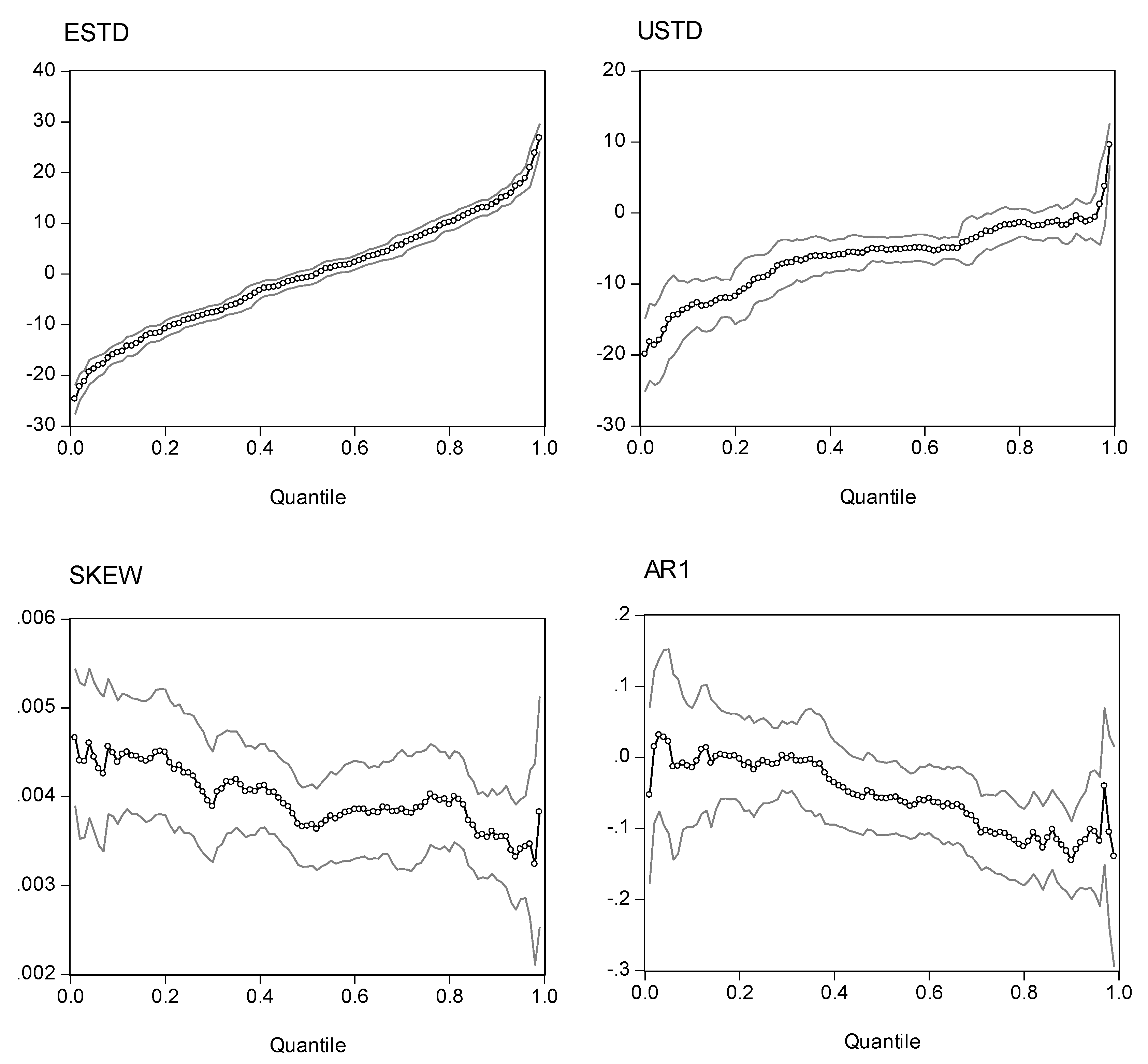
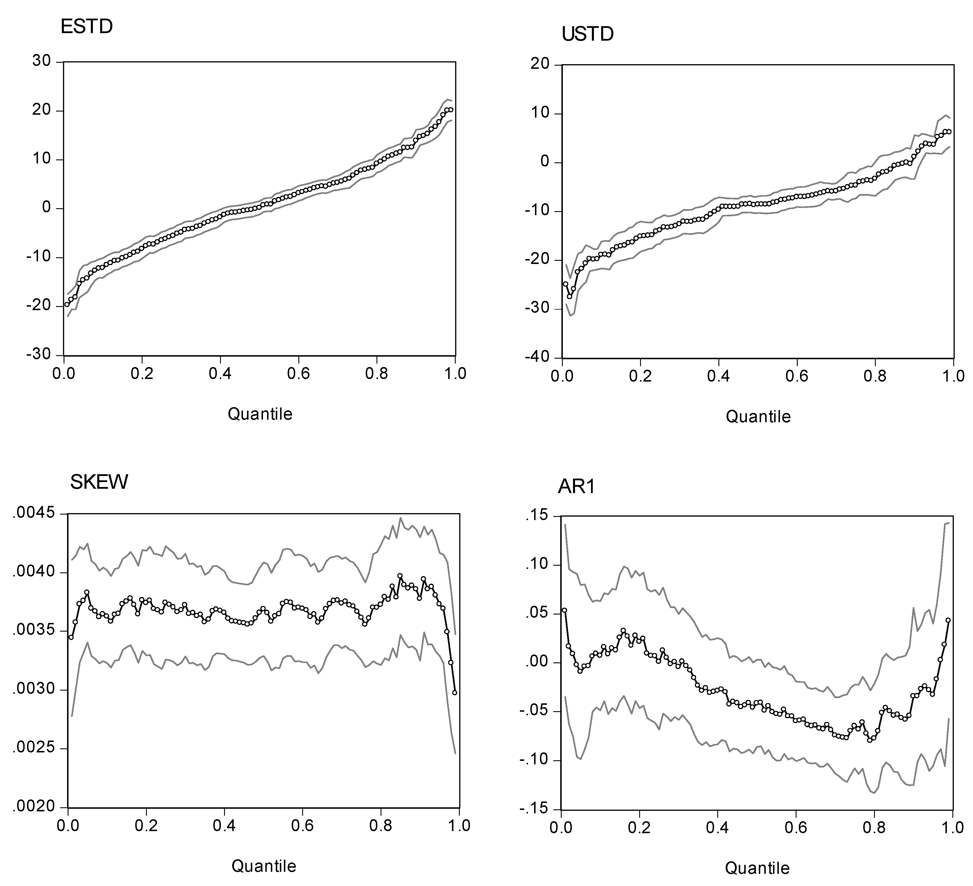
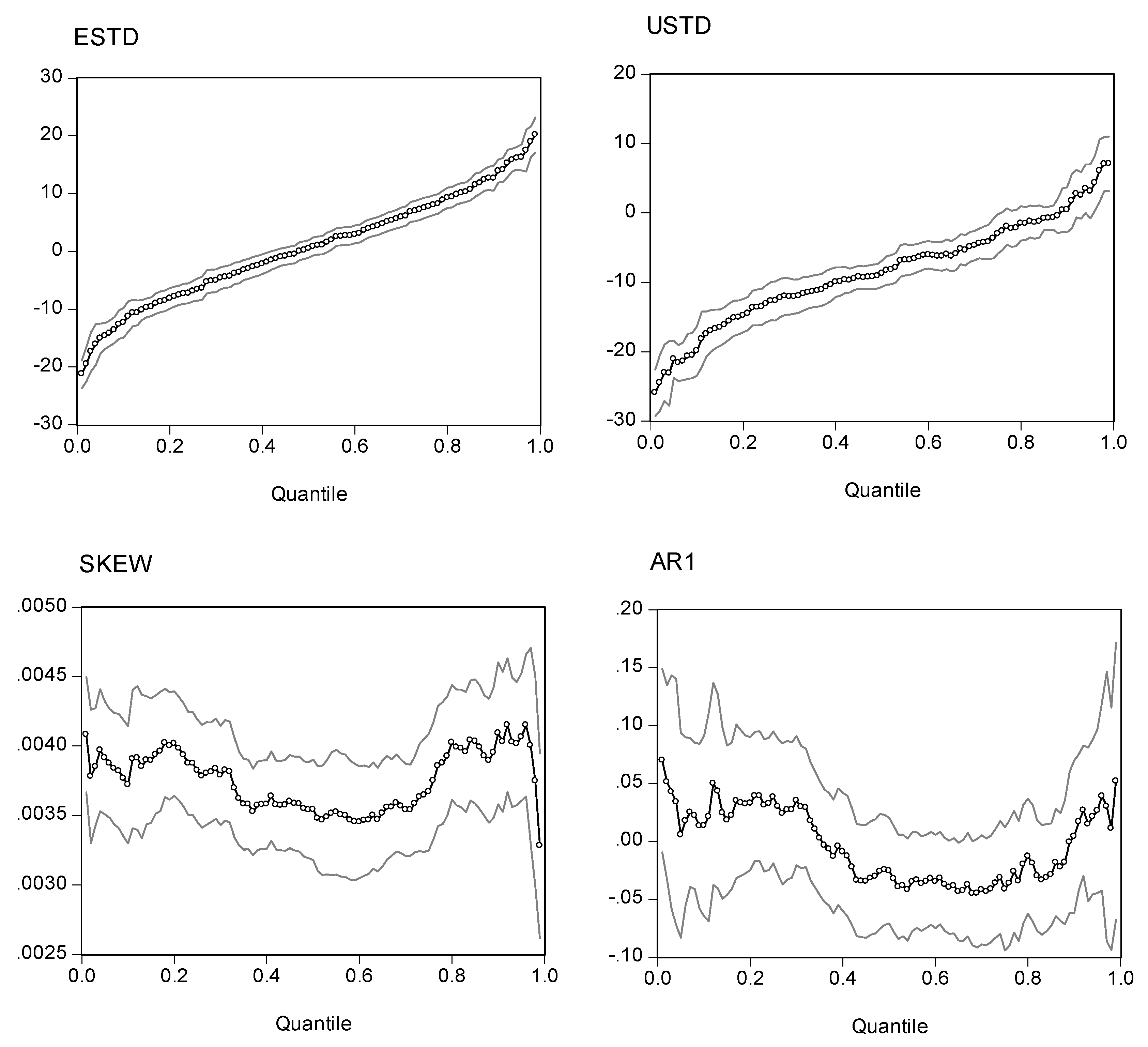
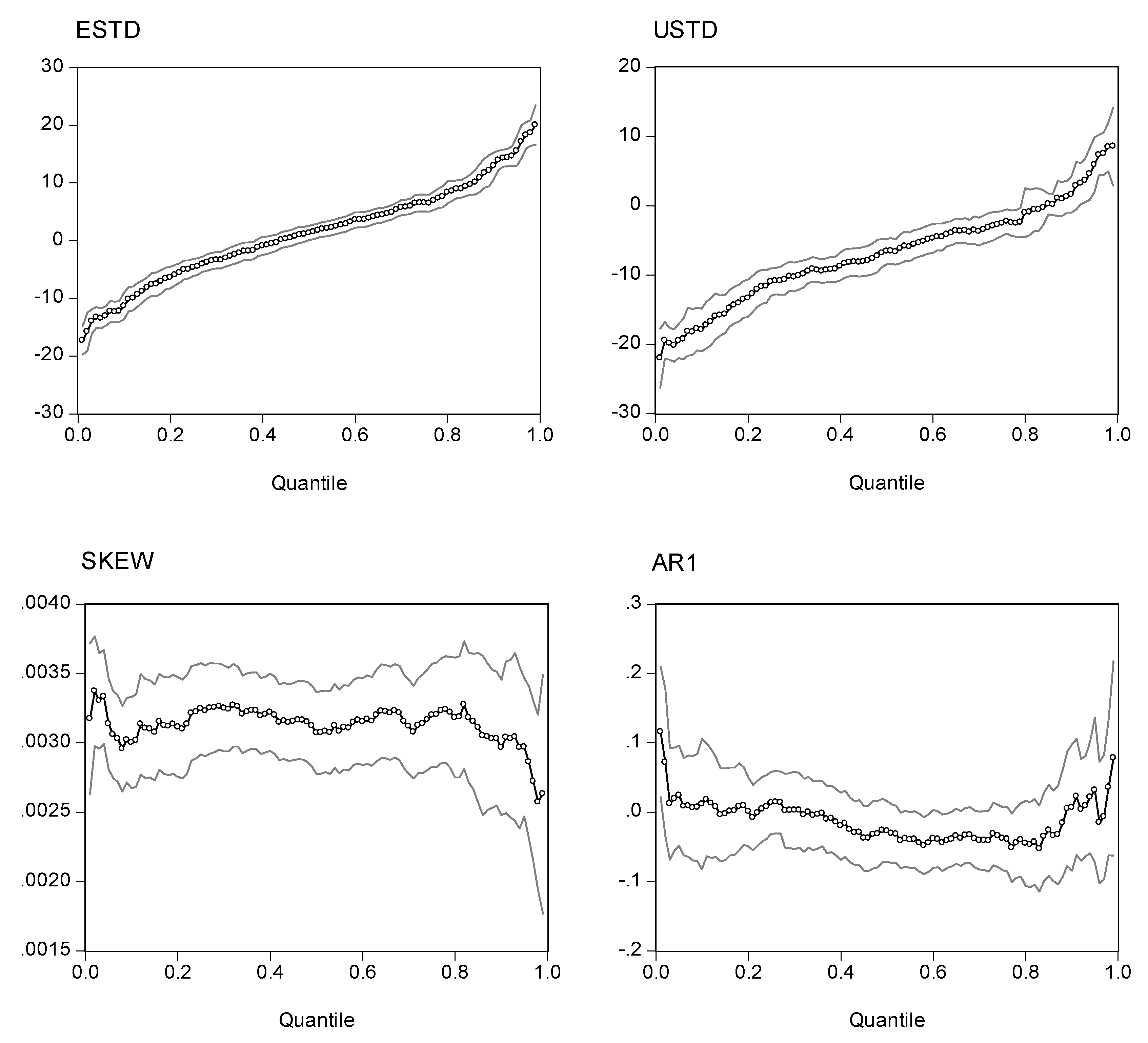
Before evaluating the statistics of the quantile regression estimations, it is more elucidative to inspect the plots of the point estimators with different quantiles. Presented in Figs. 2, 3, 4, and 5 are the estimated coefficients of the independent variables with a range of quantiles from 0.05 to 0.95 for the four indexes, which we obtain by running the regression model in Eq. (14). Each figure contains four panels, and each panel depicts point estimators for the slope of the explanatory variable along with a 95% pointwise confidence band. The vertical axis measures the magnitude of the coefficient and the horizontal, the quantiles. The plots show that the coefficient of the expected risk variable in the quantile regression is an upward function of the quantiles of the excess returns (the small-circle connected line in the panel charts). The relation between excess returns and expected risk evolves from negative to positive as the quantile increases. At lower quantiles, excess return is negatively related to expected risk; at higher quantiles, excess return is positively related to expected risk. Around the median, excess return is not correlated with expected risk, and the associated t-value is insignificant for the median regression.
We also plot the coefficients for three other explanatory variables in the figures. As with the coefficient in the expected standard deviation, the coefficient of the unexpected standard deviation increases with the quantile distributions. However, most of the estimated coefficients are in the negative zone, with minor exceptions in the upper tail of the conditional distributions. If we take the S&P 500 as an example, the coefficients are in the range (-20, 5). For quantiles lower than 0.81, the coefficients are negative; for quantiles higher than 0.92, the coefficients are positive; for quantiles between (0.81, 0.92), the coefficient is insignificant.
Turning to the intraday skewness variable, we find that the coefficients are consistent throughout the entire spectrum of quantiles. The coefficients are stable and always stay in a narrow positive regime irrespective of the quantile distributions being evaluated. This finding strengthens our earlier report that excess returns are positively related to intraday skewness.
With respect to the coefficients of the lagged index return variable (AR(1) term), those curves show a downward trend or a U-shape curve as the quantile increases. The coefficients stay in the negative zone for most of the distributions and reach a minimum level around the 80% quantile. This finding is consistent with our earlier evidence that the AR(1) coefficient in the WLS estimates has a negative value and that there is some disparity with coefficients from the GARCH model. However, at the two ends of the quantiles, we find that the AR(1) coefficients are positive (except for the NASDAQ 100 index). This finding implies that in the scenarios with more extreme movements of stock returns, there is a tendency toward moving in the same direction on the following day. However, as may be seen in the following section, the evidence shows that with the exception of the coefficients on the return of the NASDAQ 100 index in the upper tail, we find that most of the estimates are statistically insignificant. Thus, in general, we can conclude that there is a negative autocorrelation.
Table 6 reports the coefficients for the four indexes at five different quantiles (0.05, 0.25, 0.5, 0.75, and 0.95).14 As the returns on the S&P 500 index show, the estimated coefficients for the expected risk variable are -14.63, -6.46, 7.28, and 16.75 for the 0.05, 0.25, 0.75, and 0.95 quantiles, respectively. All estimates are highly significant at conventional levels. Note that all estimates of these four quantiles are significantly different from that of the median quantile (which is 0.15 with a t-value of 0.20) in both the magnitude of the coefficient and statistical significance. This pattern also reveals itself in other three indexes: significantly negative at lower quantiles but significantly positive at higher quantiles. The coefficient for the median is typically insignificant (except for the Dow Jones Industrial Average 30). This finding implies that, in general, there is no correlation between the median of excess returns and expected risk. This also suggests that the single coefficient derived by a mean regression can obscure important results. The conditional expectation represents the average relation, which can be significantly different from quantile effects. It is evident from the figures that the positive and negative impacts on the tails cancel each other out, leaving very little effect on the mean.
As shown in the panels located in the northeastern quadrants of Figs. 2-5, most of the estimated coefficients for the unexpected volatility are negative, with a few minor exceptions in the 0.95-quantile distribution. The intraday skewness coefficients consistently display a positive value and are significant at the conventional levels. Negative autocorrelation is more apparent in a more volatile stock index, NDXX. An interesting finding is that the negative coefficient is more significant at the high quantiles. Particularly, we find strong evidence of a mean reversion for the NDXX at quantile 0.5 and higher. For the low quantile regime, no mean reversion has been observed. This finding provides important evidence for clarifying the sign of the autoregression of stock returns.
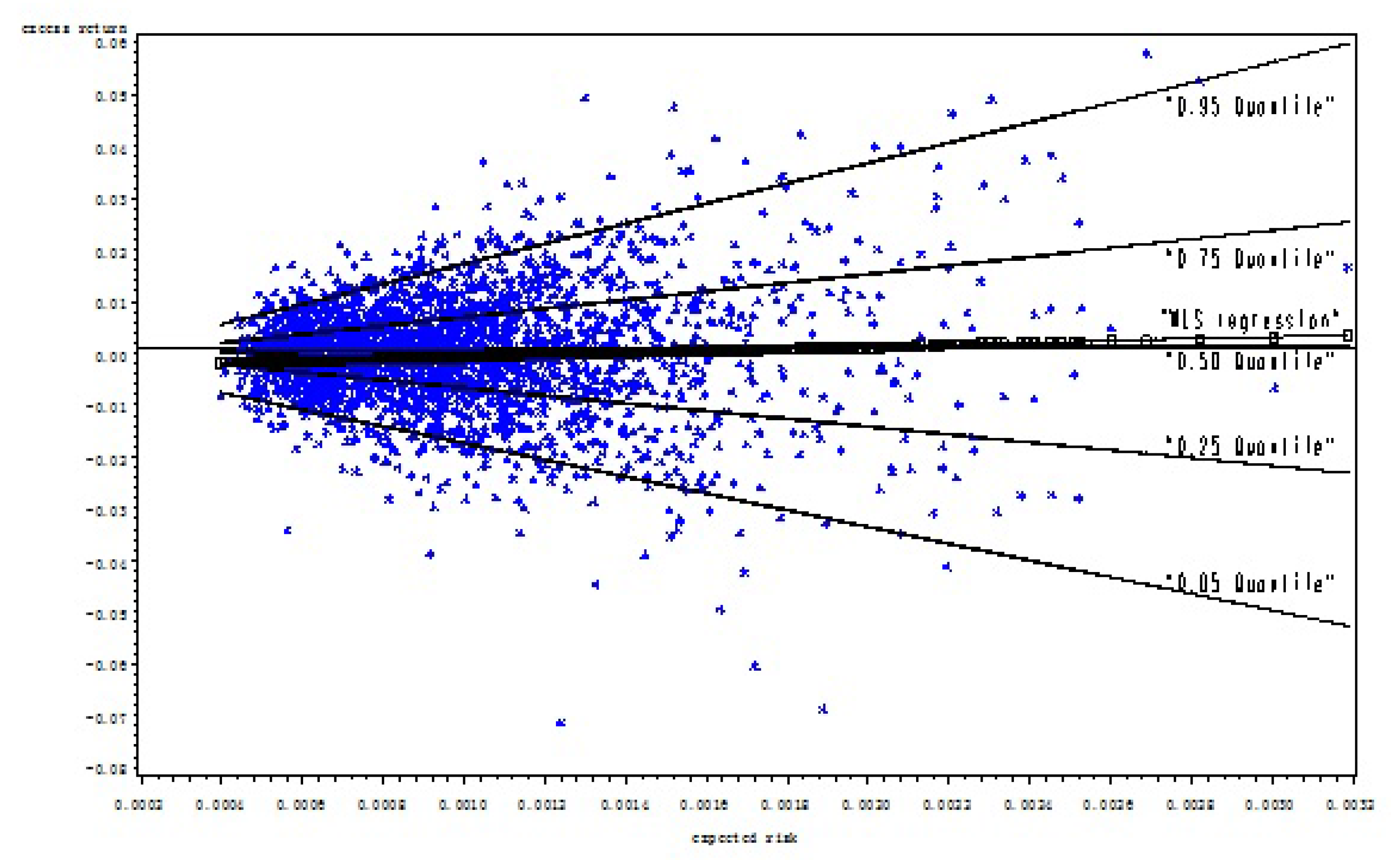
We can further illustrate the difference between least squares regression and quantile regressions that uses a simpler risk-return model. Fig. 6 shows the scatter plots between the excess return and risk variables for the S&P 500 index. Those plots form a cone or comet shape, suggesting that as risk increases, returns display a greater range of dispersion. The fitted WLS regression from Eq. (2) displays a minor upward slope, which is different from a horizontal line at the 1% significance level. However, if we compare the WLS line with the scatter plots, it is apparent that the positive risk-return relation derived from a mean-regression model is rather trivial. It fails to cover the entire spectrum of the risk-return relation.
This finding becomes clear if we compare the mean regression line with the lines derived from the quantile regression estimates. In Fig. 6, we present the quantile regression lines labeled 0.05, 0.25, 0.5, 0.75, and 0.95, respectively. The quantile regression lines labeled 0.05 and 0.25 fall below the mean/median lines, presenting a negative slope, while the regression lines labeled 0.95 and 0.75 quantiles lie above the mean/median lines, showing a positive slope.15 The risk-return relation evolves from negative to positive as the quantile increases.
Indeed, the WLS regression produces only one estimate; it provides very limited information about the risk-return relation. In contrast, a collection of conditional quantile regressions provides much more complete statistical information on the functional relations between dependent and independent variables and yields more robust results against possible outliers.
If we focus on the risk-return relation, it is tempting to ask: what is the underlying economic meaning of the sign-switching phenomenon from low to high conditional quantile distributions? Our interpretation is as follows. When economic conditions induce an optimism that corresponds to the return distributions in the upper quantiles, investors anticipate that the expected higher volatility will be compensated by the expected higher return. However, when the market is dominated by a pessimism that, in general, corresponds to the return distributions in the lower quantiles, investors perceive that high volatility will create more uncertainty, causing stock returns to fall. Thus, we observe a negative relation between excess return and expected volatility. In the median range of return quantiles, investors lack clear-cut information or fail to visualize market conditions. This ambivalent return and uncertainty render a vague risk-return relation. Our evidence suggests that when the excess return is expected to be relatively high, the risk-return hypothesis is likely to be established. However, when the excess return is expected to be low or negative, there is no tradeoff. This study also concludes that the tradeoff hypothesis does not apply to the median return.
Our empirical finding on the risk-return relation is consistent with the experience of the sub-prime crisis in the US market that started in early 2007. In this crisis, large numbers of sub-prime borrowers are at risk of defaulting on their loans, causing severe credit risk and having a cascading effect on credit markets. This perceived uncertainty is expected to cause greater volatility in stock returns, accompanied by a big loss for financial intermediaries. Under these scenarios, expected excess returns and expected volatility in stock markets are negatively correlated, since the returns are expected to be distributed to the low quantile (tail). In fact, when a big loss is anticipated in that < 0, it is hard to imagine that we can have γ > 0 in equation (1), since cannot be negative. Thus, Merton’s proposition of a risk-return tradeoff can survive only in the regime where expected excess returns are in positive territory. If we look at a long horizon, expected excess returns are anticipated to be positive because of economic growth. The tradeoff is possibly established, and this argument is consistent with the neoclassical long-run framework. However, in the short run, especially under the pessimistic market conditions, the data are not likely to confirm the tradeoff hypothesis. This argument is consistent with the study by Lundblad, who finds that “small-sample inference is plagued by the fact that conditional volatility has almost no explanatory power for realized returns.”
4.3. Test of Quantile Regression Coefficients
Although it seems obvious that the estimated coefficients vary with the quantile levels reported in Table 6, we have superimposed five estimated linear conditional quantile functions on the data. It would be more compelling if we conduct a formal test of the hypothesis of the equality of slopes. Since the median quantile is close to the mean value of the least squares estimation that has been conventionally used in testing the risk-return relation, we shall address the equality test of various quantiles against the median quantile coefficient (). Specifically, we test:
Table 7 reports the statistics for testing the null hypothesis of the equality of slopes. The Wald statistics show that the null is uniformly rejected on the coefficients of the expected risk variable at different quantile distributions, suggesting that the estimated coefficients for the quantiles of 0.05, 0.25, 0.75, and 0.95 are significantly different from that of the median distribution. The testing results point to the caveat about using a mean or median level of the data to examine the risk-return relation. The evidence suggests that the validity of the risk-return tradeoff occurs only in the upper tails, showing a significant difference from those derived from the median quantile. Thus, using the mean/median regression in the test equation tends to result in a loss of efficiency, which renders the testing results insignificant. Similar to that of the expected risk variable, the Wald statistics for the unexpected risk variable reach a parallel conclusion. Specifically, the coefficients at quantiles 0.95, 0.75, 0.25, and 0.05 are significantly different from those of the median.16 Nonetheless, for the coefficients of intraday skewness and the AR(1) term, we cannot find strong evidence against the equality of the slopes between quantiles.
In addition to the evidence that the estimated coefficients deviate from the median quantile, we are also concerned about the symmetry of the risk-return relation for the quantiles that lie above the median vs. those that lie below the median. In particular, we test the following restrictions:
Test results are reported in Table 8, where we find very little evidence of a departure from symmetry. The symmetry hypothesis cannot be rejected for the pair of (0.25, 0.75) and the pair of (0.05, 0.95) for the expected risk variable in all indexes. The risk-return relation from the quantile regression method is symmetric to the median. The other three variables’ coefficients also show symmetry except that the Russell 2000 index and the NASDAQ 100 index show little asymmetry for the intraday skewness coefficient variable at the 5% level of significance.
The symmetry property is more transparent by inspecting the plots between excess returns and standard deviations for the S&P 500 index. In Fig. 6, it is easy to see that the pair-wise quantiles (0.05, 0.95) and (0.25, 0.75) are mainly symmetrical using the median quantile as a reference.17 An implication of this test is that variance or standard deviation is still a crucial factor in modeling stock return. However, to validate the risk-return trade-off hypothesis, risk variables should be restricted to certain appropriate ranges.
5. CONCLUSION
This paper systematically investigates the risk-return relation by exploring the information derived from high-frequency data. We adopt an ARMA process to forecast expected risk proxied by the expected intraday standard deviation. The evidence suggests that daily excess returns are positively related to the expected risk for the S&P 500, the Russell 2000, and the Dow Jones Industrial Average 30 indexes, but not for the NASDAQ 100 index. The robustness test suggests that the risk-return tradeoff hypothesis is rather weak: the significant relation vanishes for the 1997-1999 sub-period and the 2004-2007 sub-period. Estimating the risk-return relation by using conventional asymmetric GARCH(1,1)-type models finds that only the DJIA index displays a significant relation, indicating the deficiency of using closing data based on a GARCH-type conditional variance model.
Consistent with the literature, the unexpected component of volatility is typically negative and highly significant. A by-product of our analysis suggests that intraday skewness, which also serves as a control variable, is highly significant in explaining the variations in daily excess returns. The evidence suggests that intraday information, both unexpected volatility and skewness, explains the stock returns very well because of the information content for return distributions revealed in intraday news and preferences.
By employing a quantile regression to analyze the data on excess returns, we find that both unexpected volatility and intraday skewness yield very stable and consistent results across different quantiles. However, the coefficient of expected returns in the test equation evolves from negative to positive as the quantile increases, and the t-statistics are significant for both the upper and lower quantiles and insignificant for the median quantile. This finding is consistent with the notion that the least squares estimators based on the conditional mean lack robustness because of the loss of information in the upper and lower tails. This is the very reason for the insignificant or conflicting signs on the risk-return relation. Our test suggests that the so-called risk-return tradeoff occurs only in the upper quantile distributions. In fact, the quantile regression results from this study suggest that both upper and lower quantiles show a significant relation between excess returns and risk.
Our study reconciles the current debate on the tradeoff hypothesis. When economic conditions are optimistic, which corresponds to the return distributions in upper quantiles, investors anticipate that the expected higher volatility will be compensated by expected higher returns. Empirically, this tradeoff can also be valid in the long run for a growing economy. However, when the market is dominated by pessimism, which, in general, corresponds to return distributions that are in the lower quantiles, investors perceive that high volatility will create more uncertainty, causing stock returns to fall. Thus, we observe a negative relationship between excess return and expected volatility. In the median range of return quantiles, investors lack clear-cut information or fail to visualize market conditions. This ambivalent return and uncertainty render a vague risk-return relation.
ACKNOWLEDGEMENTS
We have benefited from conversations and comments from Daniel Dorn, Federico Bandi, Eric Ghysels, Kevin Sheppard, Michael J. Gombola, and discussions with participants at the 2008 Society for Financial Econometrics Inaugural Conference. We assume full responsibility for the analysis and the remaining errors.
References
- A. Antoniou, G. Koutmos, and A. Pericli. “Index futures and positive feedback trading:Evidence from major stock exchanges.” Journal of Empirical Finance 12 (2005): 19–38. [Google Scholar]
- M. Barnes, and A.W. Hughes. “A Quantile Regression Analysis of the Cross Section of Stock Market Returns.” 2002. Available at SSRN: http://ssrn.com/abstract=458522.
- T. Andersen, T. Bollerslev, F. Diebold, and P. Labys. “Modeling and forecasting realized volatility.” Econometrica 71 (2003): 579–625. [Google Scholar]
- D. Backus, and A. Gregory. “Theoretical relations between risk premiums and conditional variance.” Journal of Business and Economic Statistics 11 (1993): 177–185. [Google Scholar]
- R. Baillie, and R. DeGennaro. “Stock returns and volatility.” Journal of Financial and Quantitative Analysis 25 (1990): 203–214. [Google Scholar]
- T. Bali, and L. Peng. “Is There A Risk-Return Tradeoff? Evidence from highfrequency data.” Journal of Applied Econometrics 21 (2006): 1169–1198. [Google Scholar]
- T. Bollerslev, R. Y. Chou, and K. F. Kroner. “ARCH modeling in finance: A review of the theory and empirical evidence.” Journal of Econometrics 52 (1992): 5–59. [Google Scholar]
- T. Bollerslev, and J. Wright. “High-frequency data, frequency domain inference, and volatility forecasting.” Review of Economics and Statistics 83 (2001): 596–602. [Google Scholar]
- M. Brandt, and Q. Kang. “On the relationship between the conditional mean and volatility of stock returns: A latent VAR approach.” Journal of Financial Economics 72 (2004): 217–257. [Google Scholar]
- W. Breen, L. Glosten, and R. Jagannathan. “Economic significance of predictable variations in stock index returns.” Journal of Finance 44 (1989): 1177–1189. [Google Scholar]
- J. Campbell. “Stock returns & the term structure.” Journal of Financial Economics 18 (1987): 373–399. [Google Scholar]
- J. Campbell, and L. Hentschel. “No news is good news: An asymmetric model of changing volatility in stock returns.” Journal of Financial Economics 31 (1992): 281–318. [Google Scholar]
- L. Cappiello, R. F. Engle, and K. Sheppard. “Asymmetric dynamics in the correlations of global equity and bond returns.” Journal of Financial Econometrics 4 (2006): 537–572. [Google Scholar]
- C. Chen. An Introduction to quantile regression and the QUANTREG procedure. 2006, pp. 213–30. Cary, NC: SAS Institute Inc. [Google Scholar]
- T. C. Chiang, J. Li, and L. Tan. “Empirical investigation of herding behavior in Chinese stock markets: Evidence from quantile regression analysis.” Global Finance Journal 21, 1 (2010): 111–124. [Google Scholar]
- F. Diebold. “The Nobel memorial prize for Robert F. Engle.” Scandinavian Journal of Economics 106 (2004): 165–185. [Google Scholar]
- R. Engle. “ARCH: Selected Readings.” New York, NY: Oxford University Press, 1995. [Google Scholar]
- M. Fratzscher. “Financial market integration in Europe: on the effects of EMU on stock markets.” International Journal of Finance and Economics 7 (2002): 165–193. [Google Scholar]
- K. French, W. Schwert, and R. Stambaugh. “Expected stock returns and volatility.” Journal of Financial Economics 19 (1987): 3–29. [Google Scholar]
- G. Gennotte, and T. Marsh. “Variations in economic uncertainty and risk premiums on capital assets.” European Economic Review 37 (1993): 1021–1041. [Google Scholar]
- E. Ghysels, P. Santa-Clara, and R. Valkanov. “There is a risk-return tradeoff after all.” Journal of Financial Economics 76 (2005): 509–548. [Google Scholar]
- L. Glosten, R. Jagannathan, and D. Runkle. “Relationship between the expected value and the volatility of the nominal excess return on stocks.” Journal of Finance 48 (1993): 1779–1802. [Google Scholar]
- P. Harrison, and H. Zhang. “An investigation of the risk and return relation at long horizons.” Review of Economics and Statistics 81 (1999): 399–408. [Google Scholar]
- C. R. Harvey, and A. Siddique. “Autoregressive conditional skewness.” Journal of Financial and Quantitative Analysis 34 (1999): 465–487. [Google Scholar]
- C. R. Harvey, and A. Siddique. “Conditional skewness in asset pricing tests.” Journal of Finance 55 (2000): 1263–1295. [Google Scholar]
- C. R. Harvey. “The specification of conditional expectations.” Journal of Empirical Finance 8 (2001): 573–637. [Google Scholar]
- R. Koenker. “Quantile Regression.” New York: Cambridge University Press, 2005. [Google Scholar]
- R. Koenker, and G. Bassett. “Regression quantiles.” Econometrica 46 (1978): 33–50. [Google Scholar]
- S. Koopman, and E. Uspensky. “The stochastic volatility in mean model: Empirical evidence from international stock markets.” Journal of Applied Econometrics 17 (2002): 667–689. [Google Scholar]
- A. Kraus, and R. Litzenberger. “Skewness preference and the valuation of risk assets.” Journal of Finance 31 (1976): 1085–1100. [Google Scholar]
- M. Lettau, and S. Ludvigson. “Measuring and modeling variation in the risk-return tradeoff.” In Handbook of Financial Econometrics. Edited by Y. Ait-Sahalia and L. Hansen. Amsterdam: North-Holland, 2002. [Google Scholar]
- W. K. Li, S. Ling, and M. McAleer. “Recent theoretical results for time series models with GARCH Errors.” In Contributions to Financial Econometrics. Edited by M. McAleer and L. Oxley. Malden, MA: Blackwell Publishing, 2002. [Google Scholar]
- K. G. Lim. “A new test of the three-moment capital asset pricing model.” Journal of Financial and Quantitative Analysis 24 (1989): 205–216. [Google Scholar]
- A. Lo, and C. MacKinlay. “An econometric analysis of nonsynchronous trading.” Journal of Econometrics 45 (1990): 181–211. [Google Scholar]
- C. Lundblad. “The risk return tradeoff in the long run: 1836-2003.” Journal of Financial Economics 85 (2007): 123–150. [Google Scholar]
- R. Merton. “An intertemporal capital asset pricing model.” Econometrica 41 (1973): 867–87. [Google Scholar]
- R. Merton. “On estimating the expected return on the market: An exploratory investigation.” Journal of Financial Economics 8 (1980): 323–361. [Google Scholar]
- D. Nelson. “Conditional heteroskedasticity in asset returns: A new approach.” Econometrica 59 (1991): 347–370. [Google Scholar]
- A. R. Pagan, and A. Ullah. “The econometric analysis of models with risk terms.” Journal of Applied Econometrics 3 (1988): 87–105. [Google Scholar]
- J. Scruggs. “Resolving the puzzling intertemporal relation between the market risk premium and conditional market Variance: A two-factor approach.” Journal of Finance 52 (1998): 575–603. [Google Scholar]
- E. Sentana, and S. Wadhwani. “Feedback traders and stock return autocorrelations: Evidence from a century of daily data.” Economic Journal 102 (1992): 415–435. [Google Scholar]
- J. W. Taylor. “Using exponentially weighted quantile regression to estimate value at risk and expected shortfall.” Journal of Financial Econometrics 6 (2008): 382–406. [Google Scholar]
- C. Turner, R. Startz, and C. Nelson. “A Markov model of heteroskedasticity, risk, and learning in the stock market.” Journal of Financial Economics 25 (1989): 3–22. [Google Scholar]
- R. Whitelaw. “Time variations and covariations in the expectation and volatility of stock market returns.” Journal of Finance 49 (1994): 515–541. [Google Scholar]
- 1Empirically, we find evidence that the threshold significant level of the quantile for each market is slightly above, not exactly at, the median level.
- 2Using a variance other than the standard deviation to proxy expected risk in regressions leads to a very similar conclusion. Results are available upon request.
- 3The sample period is constrained by the availability of the 5-minute high-frequency data of the stock indexes under investigation.
- 4The excess stock return is the difference between the actual stock return and the short-term interest rate. The risk-free rate is measured by the three-month Treasury bill secondary market rate, which is taken from the Federal Reserve’s website: http://www.federalreserve.gov/releases/H15/data.htm#top (serial: tbsm3m). The daily risk-free rate is measured by using the annual rate divided by 360.
- 5The daily return realized volatility is the summation of squared one-period returns (for example, 5-minute returns) from t0 to t1 (t0 and t1 are the two ends of the day). Other related volatility measurements include the summation of squared one-period returns plus the products of adjacent returns due to nonsynchronous trading in French et al. (1987), and the MIDAS measurement in Ghysels et al. (2005), which puts different weights on past daily returns when calculating monthly variance. The scheme of the weights is estimated spontaneously with the mean-equation. Volatility measurements also include GARCH-type conditional volatility, implied volatility from the Black-Scholes option pricing model, and other stochastic volatility models.
- 6To save space, we present only the SPXX series. The presentation of the other series is available upon request.
- 7A similar result is achieved by using a Newey-West consistent estimator.
- 8It would be more informative if we could directly apply a variable that proxies for investment sentiments in our model. However, we argue that intraday skewness may sufficiently reflect the directional movements of investor sentiments.
- 9A number of conditional variance models in the GARCH family have been proposed in the literature. We refer to Cappiello, Engle and Sheppard (2006, p. 568-570) for details. Other types of GARCH(1,1) models were considered, including four specifications discussed by Lundblad (2007). No significant difference is found. The additional GARCH estimations are available upon request.
- 10Since the expected volatility is in connection to an asymmetric GARCH process, we do not include the unexpected volatility variable in the mean equation. This represents another difference between a GARCH type model and Eq. (4).
- 11Quantiles are a set of “cut points” that divide a sample of data into groups containing (as far as possible) equal numbers of observations. The τ th quantile is that value of the target variable distribution below which the proportion of the population is τ. For example, the median is the 0.5th quantile, the value of a distribution where 50% of the observations are below the median. Other common quantiles are a quartile, which is the 0.25th quantile – the value of a distribution where 25% of the observations are below the quartile; a quintile, which is the 0.20th quantile – the value of a distribution where 20% of the observations are below the quintile; a decile, which is the 0.10th quantile – the value of a distribution where 10% of the observations are below the decile; and a percentile, which is the 0.01th quantile – the value of a distribution where 1% of the observations are below the percentile.
- 12Now a number of software programs are available to estimate the quantile regression, including SAS® QuantReg http://support.sas.com/techsup/. STATA® (Version 10, 2007), and EView® (Version 6, 2007). This paper finds no difference in estimated results by using any one of the above-mentioned packages.
- 13Chiang, Li, and Tan (2010) apply quantile regression method to investigate herding behavior in Chinese stock market by relating stock return dispersions to extreme market conditions. They find supporting evidence of herding behavior in both A-share and B-share investors conditional on the dispersions of returns in the lower quantile region. The current paper applies quantile regression method to estimate the relation between stock return and risk factor. The risk-return relation moves from negative to positive as the returns’ quantile increases. A positive risk-return relation is valid only in the upper quantiles. Evidently, these two papers stress on different issues and apply to different contexts.
- 14To save space and for convenience in conducting statistical tests, we do not report all of the quantile distributions. However, additional information is available upon request.
- 15In particular, the risk-return relation is insignificant at the median, which almost coincides with the horizontal line in Fig. 6. Specifically, the insignificance (at the 10% significance level) zone is 0.41-0.53 for the S&P 500 index. For quantiles less than 0.41, the data show a significant negative relation between expected return and expected risk; for quantiles between 0.41 and 0.53 inclusively, the data show insignificance; for quantiles greater than 0.53, the data show a significant positive relation. If below-median quantiles are our interest — for example, when we consider the value at risk (VaR) using a 0.05 quantile — the coefficient is negative. It implies that given other conditioning variables, the higher the expected risk, the lower the quantile of the excess returns. In other words, under more volatile market conditions, the excess return is more likely to incur a big loss. Of course, it is also more likely to incur a big gain if we focus on the above-median quantiles.
- 16The only exception is the NDXX between the 0.95 and 0.5 quantiles.
- 17We also test whether the behavior of the estimated coefficient across indexes acts differently. Thus, F-statistics for examining the restriction(s) of equal coefficient vs. without the restriction(s) were performed. Our results (not reported) show no evidence that the null is rejected for the pair of the S&P500 and the Russell 2000. This holds true for both individual and joint tests. The findings suggest that S&P500 and the Russell 2000 indexes appear to be characterized by similar behavior. This evidence should not be surprising, since both indexes cover a broader range of securities and appear to be more diversified. However, as we check on the other pairs of indexes, the joint hypothesis of equal coefficients is in general rejected, indicating that the other indexes behave differently. With respect to the individual test, we find no significant evidence against the equality of the coefficient for the AR(1) term. However, the equal coefficient of expected volatility is rejected for the NASDAQ and other indexes in the lower quantiles, meaning that the NASDAQ acts quite differently from the other indexes due to its volatile nature. This phenomenon becomes more apparent as the stock returns for the NASDAQ are in the period of relatively lower range. The estimated results are available upon request.
Fig. 1.
Three Explanatory Variables Series: Expected Volatility, Unexpected Volatility, and Intraday Skewness Coefficient
Fig. 1.
Three Explanatory Variables Series: Expected Volatility, Unexpected Volatility, and Intraday Skewness Coefficient
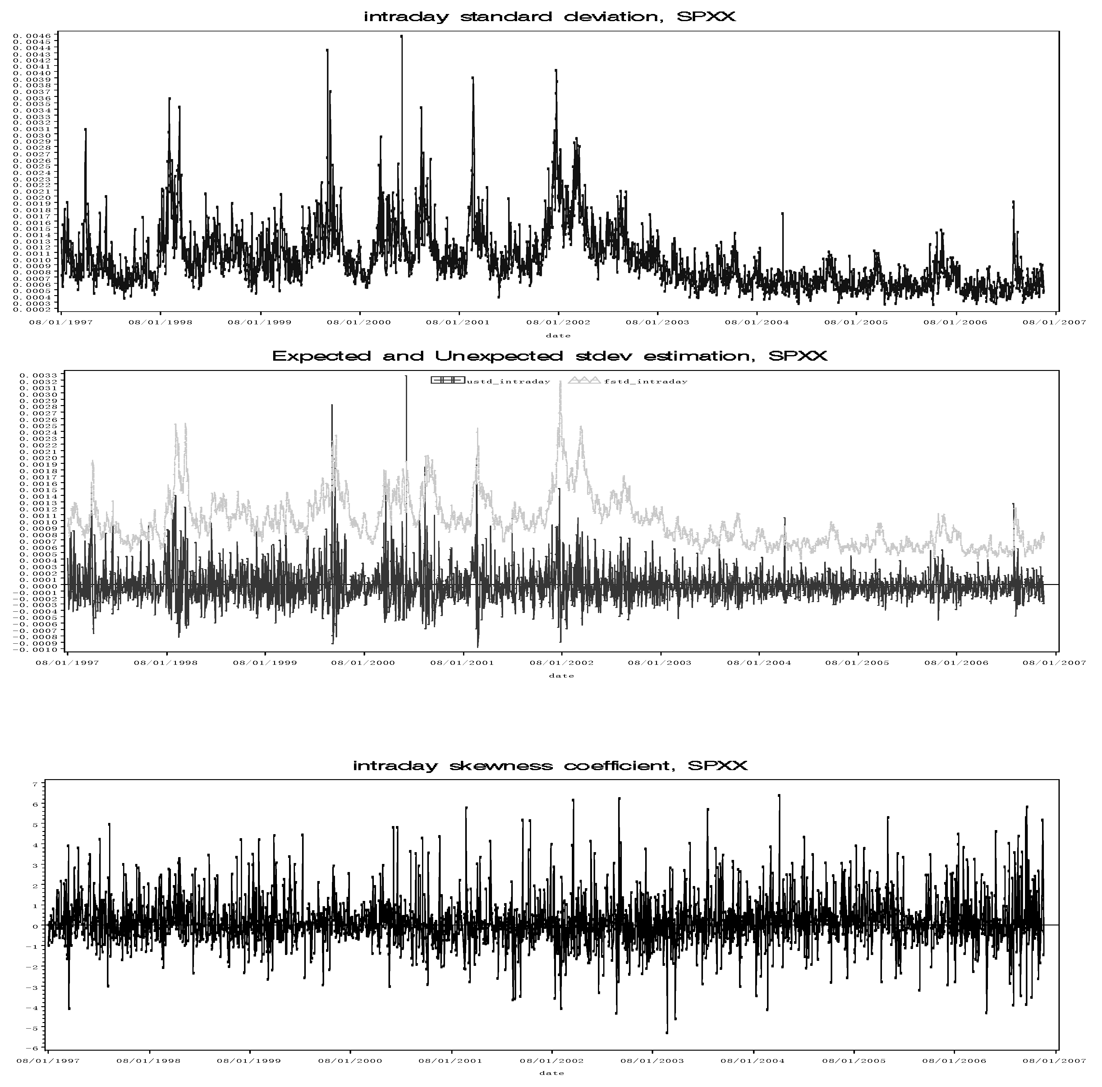
Note: These three charts are for the S&P 500 index. The top one is the intraday standard deviation. The middle one is the decomposition of the intraday standard deviation. The bottom one is the intraday skewness coefficient variable. In the middle chart, the light-colored one is the expected intraday standard deviation and the heavy-colored one is the unexpected intraday standard deviation. The unexpected intraday standard deviation has a mean value of zero by construction.
Fig. 2.
Quantile Regression Estimates (95% CI) for SPXX

Note: The quantile regression model is . The dependent variable is excess returns. The four explanatory variables are expected standard deviation (ESTD = ), unexpected standard deviation (USTD = ), the intraday skewness coefficient (Skt), and a one-period lag of the dependent variable (AR1). The charts show the estimated coefficients of the expected standard deviation, the unexpected standard deviation, and the intraday skewness variable for the of S&P 500 index. The outside lines are 95% confidence limits.
Fig. 3.
Quantile Regression Estimates (95% CI) for RUIX

Note: The quantile regression model is . The dependent variable is excess returns. The four explanatory variables are expected standard deviation (ESTD = ), unexpected standard deviation (USTD = ), the intraday skewness coefficient (Skt), and a one-period lag of the dependent variable (AR1). The charts show the estimated coefficients of the expected standard deviation, the unexpected standard deviation, and the intraday skewness variable for the Russell 2000 index. The two outside lines are 95% confidence limits.
Fig. 4.
Quantile Regression Estimates (95% CI) for NDXX
Note: The quantile regression model is . The dependent variable is excess returns. The four explanatory variables are expected standard deviation (ESTD = ), unexpected standard deviation (USTD = ), the intraday skewness coefficient (Skt), and a one-period lag of the dependent variable (AR1). The charts show the estimated coefficients of the expected standard deviation, the unexpected standard deviation, and the intraday skewness variable for the NASDAQ 100 index. The two outside lines are 95% confidence limits.
Fig. 5.
Quantile Regression Estimates (95% CI) for DJIA

Note: The quantile regression model is . The dependent variable is excess returns. The four explanatory variables are expected standard deviation (ESTD = ), unexpected standard deviation (USTD = ), the intraday skewness coefficient (Skt), and a one-period lag of the dependent variable (AR1). The charts show the estimated coefficients of the expected standard deviation, the unexpected standard deviation, and the intraday skewness variable for the Dow Jones Industrial Average 30 index. The two outside lines are 95% confidence limits.
Fig. 6.
The Predicted Value Line Using A WLS Regression

Note: The stars in the chart represent the scatter plot of expected risk and excess returns of the S&P500 index. The vertical axis is the excess returns. The horizontal axis is the expected risk variable. The thin black horizontal line represents the mean value of excess returns, which is 0.0000937. This chart shows that the risk return scatters in a parabolic comet shape. The line linked by squared legend represents the predicted value line from a WLS regression. The thin lines represent five quantile regressions. The regression model is: . The dependent variable is excess returns of the S&P500 index. The explanatory variable is the expected standard deviation () only. Estimations are reported below:
| R2/pseudo R2 | Intercept | t-value | Slope | t-value | |
| WLS mean regression | 0.23% | -.001291** | -2.08 | 1.407918** | 2.39 |
| 0.05 quantile | 12.20% | -.0012514 | -0.90 | -16.1940*** | -12.06 |
| 0.25 quantile | 2.32% | .0007371 | 0.79 | -7.50131*** | -6.77 |
| 0.5 quantile | 0.01% | .0000567 | 0.07 | .434705 | 0.43 |
| 0.75 quantile | 3.99% | -.0014044 | -1.50 | 8.306148*** | 6.77 |
| 0.95 quantile | 20.04% | -.0022981* | -1.73 | 19.48579*** | 11.13 |
This chart suggests that the risk-return relation is positive and statistically significant at the mean level but varies from negative to positive when quantile increases.

| Index | Mean | Std | Sk | Kurt | Min | Max | JB | Q2(10) | Q(10) |
|---|---|---|---|---|---|---|---|---|---|
| SPXX | 9.37E-05 | 0.011279 | -0.09051 | 3.314252 | -0.07141 | 0.057738 | 1131.92*** | 256.4658*** | 601.8206*** |
| RUIX | 8.84E-06 | 0.010663 | -0.18446 | 3.410984 | -0.0686 | 0.056702 | 1208.721*** | 291.3726*** | 700.7981*** |
| NDXX | 0.000127 | 0.021943 | 0.178606 | 4.035045 | -0.1037 | 0.17228 | 1691.348*** | 404.5428*** | 1079.626*** |
| DJIA | 0.000106 | 0.010977 | -0.21035 | 4.347062 | -0.07481 | 0.061501 | 1960.266*** | 267.022*** | 563.2825*** |
Note 1: This table provides a summary of statistics for four daily index excess returns: 1997-2007.
Note 2: The statistics of stock index returns in columns are mean, standard deviation, skewness, excess kurtosis, minimum value, maximum value, and Jarque-Bera (JB) statistic for testing normality. Q2(10) is the Ljung –Box statistics for testing autocorrelations of stock returns squared up to the 10th order. The rejection of null implies the existence of heteroskedasticity of stock returns; the Q(10) is the Portmanteau test for examining autocorrelations of returns up to 10th order. The index returns in the sample are S&P 500 (SPXX), Russell 2000 (RUIX), NASDAQ 100 (NDXX), and Dow Jones Industrial Average 30 (DJIA). Each index has 2,485 observations. *** indicates significance at the 1% level.
| Index | Expected risk () | ||||||||
| mean | std | t-value | min | max | |||||
| SPXX | 0.00098344** | 0.00038459 | (2.55) | 0.00039656 | 0.00318790 | ||||
| RUIX | 0.00092344*** | 0.00034727 | (2.66) | 0.00038376 | 0.00300001 | ||||
| NDXX | 0.00177362** | 0.00087211 | (2.03) | 0.00060273 | 0.00624109 | ||||
| DJIA | 0.00103098*** | 0.00040089 | (2.58) | 0.00040471 | 0.00332588 | ||||
| Index | Unexpected risk () | ||||||||
| mean | std | t-value | min | max | |||||
| SPXX | 1.48E-06 | 0.00029668 | (0.25) | -0.0009764 | 0.00327197 | ||||
| RUIX | 2.85E-06 | 0.0002751 | (0.52) | -0.0008448 | 0.00277801 | ||||
| NDXX | 8.95E-06 | 0.00056891 | (0.78) | -0.0023822 | 0.0061042 | ||||
| DJIA | 9.09E-07 | 0.00032073 | (0.14) | -0.0012559 | 0.0035319 | ||||
| Index | Intraday Skewness Coefficient (Skt) | ||||||||
| mean | std | t-value | min | max | |||||
| SPXX | 0.1748743*** | 1.20475523 | (7.24) | -5.271835 | 6.3970447 | ||||
| RUIX | 0.1550598*** | 1.19580593 | (6.46) | -6.0180115 | 6.6392911 | ||||
| NDXX | 0.1950596*** | 1.48590321 | (6.54) | -7.6282694 | 7.62555013 | ||||
| DJIA | 0.2079446*** | 1.4200072 | (7.30) | -5.4788261 | 6.89371099 | ||||
| Pearson’s Correlation Coefficients | |||||||||
| Index | & | & Skt | & Skt | ||||||
| SPXX | 0.0103294 | 0.0188583 | -0.0382485 | ||||||
| RUIX | 0.0219334 | 0.0043186 | -0.0586303 | ||||||
| NDXX | 0.0057106 | 0.0301476 | -0.072874 | ||||||
| DJIA | 0.0143635 | -0.0259234 | -0.0229389 | ||||||
Note: This table describes the mean, standard deviation, minimum, and maximum of the three explanatory variables: expected standard deviation of index returns, , unexpected standard deviation of index returns,, and intraday skewness coefficient of index returns, Skt. t-value tests if the mean is statistically different from zero. ***, **, and * denote statistical significance at the 1%, 5%, and 10% levels, respectively. The unexpected standard deviation has a zero mean according to its construction. The table also reports the Pearson’s correlation coefficients among the three variables. The three variables have very small correlation coefficients among them. The samples are S&P 500 (SPXX), Russell 2000 (RUIX), NASDAQ 100 (NDXX), and Dow Jones Industrial Average 30 (DJIA).
Table 3.
Regression Results of Excess Returns on Expected Volatility Using A WLS Regression Model
| Index | ||||||
| SPXX | -0.003*** | 1.876*** | - | - | - | 0.31% |
| (-3.31) | (2.96) | - | - | - | ||
| RUIX | -0.003*** | 1.926*** | - | - | - | 0.32% |
| (-3.52) | (2.98) | - | - | - | ||
| NDXX | -0.002 | 0.563 | - | - | - | 0.001% |
| (-1.42) | (1.00) | - | - | - | ||
| DJIA | -0.002*** | 1.668*** | - | - | - | 0.28% |
| (-3.10) | (2.84) | - | - | - |
| SPXX | -0.003*** | 2.468*** | -6.223*** | - | - | 3.49% |
| (-3.49) | (3.94) | (-9.09) | - | - | ||
| RUIX | -0.003*** | 2.738*** | -7.579*** | - | - | 4.71% |
| (-3.87) | (4.31) | (-10.75) | - | - | ||
| NDXX | -0.002 | 0.777 | -2.432*** | - | - | 0.46% |
| (-1.42) | (1.37) | (-3.55) | - | - | ||
| DJIA | -0.002*** | 2.216*** | -5.618*** | - | - | 3.45% |
| (-3.26) | (3.81) | (-9.07) | - | - |
| SPXX | -0.003*** | 1.961*** | -6.789*** | 0.005*** | -0.07*** | 26.08% |
| (-4.46) | (3.57) | (-10.58) | (26.98) | (-3.69) | ||
| RUIX | -0.003*** | 2.401*** | -6.707*** | 0.005*** | -0.047** | 25.39% |
| (-4.98) | (4.27) | (-10.16) | (25.83) | (-2.53) | ||
| NDXX | -0.002 | 0.291 | -2.235*** | 0.005*** | -0.1*** | 9.82% |
| (-1.58) | (0.54) | (-3.14) | (15.04) | (-4.84) | ||
| DJIA | -0.003*** | 2.171*** | -5.23*** | 0.004*** | -0.031* | 28.13% |
| (-5.05) | (4.33) | (-9.24) | (28.93) | (-1.68) |
Note 1: This table reports the estimates by regressing the excess returns on expected volatility using a WLS regression model.
Note 2: The regression models are: (panel A), (panel B), and (panel C). The dependent variable is excess returns. The explanatory variables are expected standard deviation (), unexpected standard deviation (), intraday skewness coefficient (Skt), and a one-period lag of the dependent variable. The is the adjusted R-squared. The numbers in parenthesis are t-values of the coefficients. ***, **, and * denote statistical significance at the 1%, 5%, and 10% levels, respectively. The index returns in the sample are S&P 500 (SPXX), Russell 2000 (RUIX), NASDAQ 100 (NDXX), and Dow Jones Industrial Average 30 (DJIA). Regression results show that the coefficients of for three indexes (SPXX, RUIX, and DJIA) have a positive sign and are statistically significant. The evidence indicates that the coefficient of for all four indexes bear a negative sign and are statistically significant. With respect to panel C, in addition to producing consistent statistical results for coefficients of and , the skt variable has significant power to explain the expected excess returns for all of the indexes.
| Index | ||||||||
| SPXX | -0.0012*** | 0.0875 | 0.0033*** | 0.0443** | 0.0000*** | 0.0223* | 0.8944*** | 0.1268*** |
| (-2.83) | (1.57 ) | (27.25) | (2.32 ) | (4.23 ) | (1.95 ) | (60.91) | (5.90 ) | |
| RUIX | -0.0012*** | 0.0892 | 0.0033*** | 0.0607*** | 0.0000*** | 0.0281** | 0.8976*** | 0.1055*** |
| (-2.64) | (1.47 ) | (26.96) | (3.25 ) | (4.36 ) | (2.45 ) | (64.65) | (5.64 ) | |
| NDXX | -0.0006 | 0.0149 | 0.0034*** | -0.0126 | 0.000*** | 0.0226*** | 0.9430*** | 0.0613*** |
| (-1.15) | (0.39 ) | (24.23) | (-0.64) | (3.98 ) | (32.09) | (503.50) | (26.88) | |
| DJIA | -0.0014*** | 0.1198** | 0.0027*** | 0.0456*** | 0.0000*** | 0.0278*** | 0.9065*** | 0.1050*** |
| (-3.36) | (2.06 ) | (28.45) | (2.68 ) | (3.65 ) | (2.59 ) | (69.76) | (6.43 ) |
Note: This table provides estimates by regressing the excess returns on expected volatility using a GJR-GARCH(1,1) model. The regression model is expressed as: .The dependent variable rt in the mean equation is excess returns. The three explanatory variables are expected standard deviation (ht1/2), intraday skewness coefficient (Skt), and one-period lag of the dependent variable, rt. The error term, , is assumed to be randomly distributed with zero mean and conditional variance ht. The conditional variance follows an asymmetric GARCH(1,1) process (Glosten et al., 1993). I is an indicative function, which takes a value of unity when the condition inside the parenthesis is met, 0 otherwise. The numbers in parenthesis are t-values of the coefficients. ***, **, and * denote statistical significance at the 1%, 5%, and 10% levels, respectively. The index returns in the sample are S&P 500 (SPXX), Russell 2000 (RUIX), NASDAQ 100 (NDXX), and Dow Jones Industrial Average 30 (DJIA). A positive β1 indicates a positive relation between the excess return and conditional volatility. Regression results show that only the DJIA series shows a positive significant risk-return relation. The evidence indicates that both the coefficients of skewness and AR(1) are statistically significant. Note that the value of 0.000 shown on the coefficient of denotes a very small value.
Table 5.
Sub-Sample Estimates of the Excess Return Equation: WLS Method
| Index | ||||||
| SPXX | -0.002 | 1.049 | -13.443*** | 0.006*** | -0.234*** | 33.72% |
| (-1.03) | (0.80) | (-9.3) | (13.1) | (-6.03) | ||
| RUIX | -0.002 | 1.326 | -14.046*** | 0.005*** | -0.171*** | 34.35% |
| (-1.24) | (0.96) | (-9.25) | (13.19) | (-4.46) | ||
| NDXX | -0.002 | 0.987 | -3.442*** | 0.004*** | -0.128*** | 23.19% |
| (-0.67) | (0.65) | (-3.04) | (11.57) | (-3.34) | ||
| DJIA | -0.002 | 1.086 | -4.556*** | 0.006*** | -0.112*** | 22.50% |
| (-1.14) | (0.79) | (-3.96) | (11.93) | (-2.80) |
| Index | ||||||
| SPXX | -0.003** | 2.137** | -5.014*** | 0.006*** | -0.025 | 26.16% |
| (-2.40) | (2.06) | (-5.22) | (17.91) | (-0.85) | ||
| RUIX | -0.004*** | 2.783*** | -4.214*** | 0.005*** | -0.02 | 23.63% |
| (-2.89) | (2.69) | (-4.26) | (16.26) | (-0.70) | ||
| NDXX | -0.003 | 0.227 | -1.597 | 0.01*** | -0.089*** | 9.35% |
| (-0.87) | (0.20) | (-1.35) | (9.56) | (-2.69) | ||
| DJIA | -0.003*** | 2.185** | -5.492*** | 0.005*** | 0.006 | 33.64% |
| (-2.63) | (2.51) | (-6.21) | (21.17) | (0.20) |
| Index | ||||||
| SPXX | -0.001 | -0.18 | -7.859*** | 0.003*** | -0.021 | 32.40% |
| (-0.58) | (-0.13) | (-7.49) | (18.43) | (-0.69) | ||
| RUIX | 0 | -0.322 | -8.509*** | 0.003*** | -0.011 | 34.96% |
| (-0.50) | (-0.23) | (-8.22) | (19.73) | (-0.38) | ||
| NDXX | 0.001 | -1.081 | -6.058*** | 0.003*** | 0.005 | 20.58% |
| (0.40) | (-0.65) | (-5.32) | (13.92) | (0.15) | ||
| DJIA | -0.002** | 1.799 | -6.055*** | 0.002*** | 0.005 | 35.46% |
| (-2.14) | (1.34) | (-7.09) | (20.22) | (0.16) |
Note: This table provides sub-sample estimates of the excess return equation using a WLS method. The regression model is The dependent variable is excess returns. The four explanatory variables are expected standard deviation (), unexpected standard deviation (), the intraday skewness coefficient (Skt), and a one-period lag of the dependent variable. The is the adjusted R-squared. The numbers inside parenthesis are t-values of the coefficients. ***, **, and * denote statistical significance at the 1%, 5%, and 10% levels, respectively. The samples are SPXX: S&P 500 index, RUIX: Russell 2000 index, NDXX: NASDAQ 100 index, and DJIA: Dow Jones Industrial Average 30 index. Regression results show that three indexes (SPXX, RUIX, and DJIA) show positive significance for the σe in the regressions only in the middle period 2000-2003. The significance disappears in other periods. Mean reversion is more significant in the period 1997-1999.
| Index | Quantile | Pseudo R2 | |||||
| SPXX | 0.05 | 33.09% | -0.00038 | -14.6386*** | -21.7702*** | 0.003828*** | -0.00941 |
| (-0.31) | (-9.80) | (-11.76) | (21.69) | (-0.18) | |||
| 0.25 | 18.72% | -0.00014 | -6.46454*** | -13.8894*** | 0.003743*** | 0.000774 | |
| (-0.22) | (-8.06) | (-10.9) | (17.83) | (0.02) | |||
| 0.5 | 15.02% | -0.00067 | 0.154797 | -8.59299*** | 0.003688*** | -0.04146* | |
| (-1.11) | (0.20) | (-9.93) | (18.74) | (-1.70) | |||
| 0.75 | 17.90% | -0.00191*** | 7.277967*** | -4.71301*** | 0.003615*** | -0.06495*** | |
| (-2.60) | (7.49) | (-2.98) | (16.51) | (-2.56) | |||
| 0.95 | 32.74% | -0.00288** | 16.74875*** | 3.627727** | 0.003729*** | -0.03261 | |
| (-2.48) | (11.41) | (2.35) | (13.56) | (-0.90) | |||
| RUIX | 0.05 | 32.08% | -8.8E-05 | -15.1693*** | -21.058*** | 0.003884*** | 0.006585 |
| (-0.08) | (-11.55) | (-10.45) | (14.29) | (0.14) | |||
| 0.25 | 19.25% | 9.15E-05 | -7.01984*** | -12.9743*** | 0.003784*** | 0.026966 | |
| (0.13) | (-8.52) | (-9.06) | (21.63) | (1.06) | |||
| 0.5 | 14.72% | -0.00088 | 0.497222 | -8.91271*** | 0.003482*** | -0.02586 | |
| (-1.30) | (0.58) | (-8.84) | (19.77) | (-1.07) | |||
| 0.75 | 17.80% | -0.00197*** | 7.654579*** | -3.32788** | 0.003614*** | -0.0347 | |
| (-2.62) | (8.19) | (-2.13) | (15.19) | (-1.21) | |||
| 0.95 | 30.69% | -0.00237** | 16.26831*** | 3.018618 | 0.003945*** | 0.01987 | |
| (-2.42) | (13.25) | (1.51) | (14.3) | (0.49) | |||
| NDXX | 0.05 | 30.83% | 0.003599** | -18.7663*** | -16.4915*** | 0.004446*** | 0.022146 |
| (2.20) | (-18.15) | (-6.79) | (11.7) | (0.34) | |||
| 0.25 | 14.16% | 0.002607*** | -8.94388*** | -9.18697*** | 0.004263*** | -0.00484 | |
| (2.82) | (-12.39) | (-5.50) | (13.12) | (-0.16) | |||
| 0.5 | 7.28% | 0.001169 | -0.68442 | -5.16647*** | 0.003665*** | -0.05789** | |
| (1.07) | (-0.80) | (-4.84) | (13.09) | (-2.39) | |||
| 0.75 | 12.23% | -0.00215* | 7.976723*** | -2.28103* | 0.003933*** | -0.10602*** | |
| (-1.79) | (8.51) | (-1.76) | (10.58) | (-3.74) | |||
| 0.95 | 29.89% | -0.00468** | 17.78006*** | -1.05148 | 0.003407*** | -0.10505** | |
| (-2.45) | (12.08) | (-0.35) | (9.29) | (-2.05) | |||
| DJIA | 0.05 | 34.05% | -0.00051 | -13.4738*** | -19.4992*** | 0.003136*** | 0.024013 |
| (-0.60) | (-15.67) | (-10.71) | (24.11) | (0.66) | |||
| 0.25 | 18.96% | -0.00144** | -4.62158*** | -11.0077*** | 0.003246*** | 0.013546 | |
| (-2.08) | (-5.59) | (-9.24) | (17.6) | (0.50) | |||
| 0.5 | 14.86% | -0.00182*** | 1.311631** | -6.58008*** | 0.003105*** | -0.02528 | |
| (-3.41) | (2.10) | (-5.89) | (21.93) | (-1.09) | |||
| 0.75 | 17.09% | -0.00203*** | 6.65549*** | -2.53834** | 0.003233*** | -0.03515 | |
| (-3.05) | (8.83) | (-2.15) | (15.32) | (-1.59) | |||
| 0.95 | 28.48% | -0.00228** | 15.50437*** | 5.881941*** | 0.002978*** | 0.030173 | |
| (-2.05) | (11.67) | (3.08) | (10.78) | (0.59) |
Note: This table reports the estimates of quantile regression for different index returns. The model is: |, ) = The dependent variable is excess returns. The four explanatory variables are expected standard deviation (), unexpected standard deviation (), the intraday skewness coefficient (Skt), and an AR(1) term. The refers to the kth coefficient conditional on quantile distribution in the estimated equation. The numbers in parenthesis are t-values of the coefficients. ***, **, and * denote statistical significance at the 1%, 5%, and 10% levels, respectively. The samples are indexes of S&P 500 (SPXX), Russell 2000 (RUIX), NASDAQ 100 (NDXX), and Dow Jones Industrial Average 30 (DJIA). This table reports the pseudo R2 quantile regressions, the coefficient estimates and t-values of independent variables for the 0.05, 0.25, 0.5, 0.75, and 0.95 quantiles. Regression results show that the coefficient of the expected standard deviation () evolves from negative to positive as the quantile increases. It is insignificant at the median level except for the DJIA 30 index.
Table 7.
Equality Test of Quantile Regression Coefficients
| Index | ||||
| SPXX | 108.25*** | 72.37*** | 67.2*** | 89.69*** |
| RUIX | 155.88*** | 69.75*** | 79.28*** | 101.67*** |
| NDXX | 142.78*** | 100.22*** | 96.54*** | 192.18*** |
| DJIA | 114.62*** | 57.17*** | 62.13*** | 249.09*** |
| Index | ||||
| SPXX | 49.82*** | 8.02*** | 22.54*** | 41.91*** |
| RUIX | 32.82*** | 17.01*** | 12.33*** | 34.05*** |
| NDXX | 1.99 | 6.38** | 7.97*** | 23.73*** |
| DJIA | 44.01*** | 13.12*** | 16.17*** | 51.58*** |
| Index | ||||
| SPXX | 0.02 | 0.12 | 0.08 | 0.36 |
| RUIX | 3.07* | 0.38 | 3.49* | 2.32 |
| NDXX | 0.34 | 0.93 | 3.49* | 3.37* |
| DJIA | 0.22 | 0.51 | 0.98 | 0.03 |
| Index | ||||
| SPXX | 0.06 | 0.98 | 2.03 | 0.37 |
| RUIX | 0.88 | 0.09 | 4.70** | 0.39 |
| NDXX | 0.76 | 3.57* | 3.79* | 1.47 |
| DJIA | 1.14 | 0.18 | 2.69 | 1.66 |
Note: This table reports the equality test of quantile regression coefficients. The hypotheses are listed in the heading of the column. refers to the kth coefficient conditional on quantile distribution in the following equation: | , ) = For instance, hypothesizes that the coefficient of for 0.95 quantile is equal to the coefficient of for 0.5 quantile. The statistics are performed by F-test that follows an F(1, 2,479) distribution. The samples are indexes of S&P 500 (SPXX), Russell 2000 (RUIX), NASDAQ 100 (NDXX), and Dow Jones Industrial Average 30 (DJIA). ***, **, and * denote statistical significance at the 1%, 5%, and 10% levels, respectively. Results show that coefficients of expected risk variable at 0.95, 0.75, 0.25, and 0.05 quantiles are obviously different from that of 0.50 quantile.
Table 8.
Symmetry Test of Quantile Regression Coefficients
| Index | ||
| SPXX | 0.62 | 0.17 |
| RUIX | 0.00 | 0.07 |
| NDXX | 0.03 | 0.08 |
| DJIA | 0.12 | 0.32 |
| Index | ||
| SPXX | 0.11 | 0.61 |
| RUIX | 0.00 | 0.67 |
| NDXX | 3.76* | 0.35 |
| DJIA | 0.03 | 0.05 |
| Index | ||
| SPXX | 0.17 | 0.00 |
| RUIX | 4.73** | 2.44 |
| NDXX | 0.57 | 4.87** |
| DJIA | 0.08 | 1.17 |
| Index | ||
| SPXX | 0.40 | 0.28 |
| RUIX | 1.05 | 1.15 |
| NDXX | 0.15 | 0.02 |
| DJIA | 2.80* | 0.64 |
Note: This table reports the Wald statistics for the hypothesis testing. The null hypotheses are listed in the heading of the column. refers to the kth coefficient conditional on quantile distribution in the following equation: | , ) = . states that the coefficient for the 0.95 quantile and the coefficient for the 0.05 quantile are symmetric to the coefficient of the 0.5 quantile. Likewise, tests that the coefficients of the 0.75 quantile and the 0.25 quantile are symmetric to the coefficient of the 0.5 quantile. The Wald test formed is zero under the null hypothesis of symmetry. The statistic follows an F(1, 2,479) distribution. The samples are indexes of S&P 500 (SPXX), Russell 2000 (RUIX), NASDAQ 100 (NDXX), and Dow Jones Industrial Average 30 (DJIA). ***, **, and * denote statistical significance at the 1%, 5%, and 10% levels, respectively. Results cannot reject the hypotheses, indicating that the coefficients are symmetrical to the coefficient of the median.
Share and Cite
MDPI and ACS Style
Chiang, T.C.; Li, J. Stock Returns and Risk: Evidence from Quantile. J. Risk Financial Manag. 2012, 5, 20-58. https://doi.org/10.3390/jrfm5010020
AMA Style
Chiang TC, Li J. Stock Returns and Risk: Evidence from Quantile. Journal of Risk and Financial Management. 2012; 5(1):20-58. https://doi.org/10.3390/jrfm5010020
Chicago/Turabian StyleChiang, Thomas C., and Jiandong Li. 2012. "Stock Returns and Risk: Evidence from Quantile" Journal of Risk and Financial Management 5, no. 1: 20-58. https://doi.org/10.3390/jrfm5010020