Hedonic Price Function for Residential Area Focusing on the Reasons for Residential Preferences in Japanese Metropolitan Areas

Abstract

This study aims to offer a new estimate of the hedonic price function of residential areas in Japanese metropolitan areas, focusing on the reasons for residential preferences. More specifically, it introduces two new explanatory variables—‘regional vulnerability’ and ‘accessibility to destination stations’—and determines their usefulness. Based on the evaluation done in this study, the hedonic price function mentioned above showed 60% interpretability (as compared to 52% interpretability by hedonic price function using only conventional explanatory variables.) In addition, the significance level of both the explanatory variables was low, and the land price changed by 9% as the regional vulnerability changed by 1 grade. Furthermore, residents placed great emphasis on both variables. This made it evident that the introduction of the two explanatory variables that reflect the reasons for residential preferences specific to Japanese metropolitan areas was reasonable.

1. Introduction

Worsening financial conditions across the globe call for efficient public investment plans and correct measurement of investment effects. Land prices are an important element (Mikanagi and Morisugi 1981) in this regard. In addition, land use models that address changes in land use due to public investments show that prices play a key role in location behavior mechanism (Nakamura et al. 1981). Therefore, improvement in measurement accuracy is important in order to estimate price functions that can accurately grasp the changes in land price structure caused by public investments. The hedonic approach is generally used as a land price estimation method. It is a statistical method that can grasp how differences in environmental conditions are reflected in differences in land prices, and measure the environmental value based on such information. However, in most metropolitan areas with a mix of factors, the estimation accuracy for land prices tends to be lower.

Residential preferences in metropolitan areas is one reason why estimation accuracy for land prices tends to be lower. Local population density and rental prices tend to decrease the farther you are from the central business district (bid rent theory). This indicates that residents place importance on accessibility to the city center or the central business district. However, with development of the railway transportation system in metropolitan areas, it is necessary to focus on accessibility to and characteristics of destination stations. In addition, regional vulnerability is another reason for residential preferences—disasters can be severe in metropolitan areas and can cause largescale damage owing to overcrowding with people and workplaces. This study, thus, aims to offer a new estimate of the hedonic price function for residential area in Japanese metropolitan areas, focusing on the reasons for residential preferences, as mentioned above.

2. Related Work

The present study is categorized as an analysis of the estimation of residential land prices using the hedonic approach. The following are representative examples of studies closely related to it.

Tse (2002) estimated neighborhood effects on house prices in Hong Kong. Kim et al. (2003) developed a spatial-econometric hedonic housing price model that estimates marginal improvements in air quality in the Seoul metropolitan area. Fik et al. (2003) proposed an interactive variables approach and tested its ability to explain price variations in an urban residential housing market in Tucson, Arizona. Shimuzu (2004) estimated price functions using transaction price, with apartments as a target. Ismail (2005) developed a hedonic model of housing markets using Geographical Information System (GIS) and spatial statistics, and applied it in Glasgow, Scotland. Shimuzu and Karawatari (2007) used an estimation method focusing on spatial autocorrelation to estimate land price function in the 23 wards of Tokyo (the largest city and capital of Japan). Hill and Melser (2007) compared house prices in 14 regions of Sydney over six years, using the hedonic approach.

Kutsuzawa (2008) indicated that in the 23 wards of Tokyo, areas with higher crime rates had lower residential land prices. Aikoh et al. (2008) grasped the effects of greenery maintenance on residential land prices in Sapporo. Cohen and Coughlin (2008) compared various spatial econometric models and estimation methods in a hedonic price framework to examine the impact of noise on housing prices near the Atlanta airport. Tokuda (2009) quantitatively grasped the factors that impact residential land prices in Shiga prefecture, and indicated that around 80% of residential land prices can be expressed using Equation (1):

$$\begin{gathered} \mathrm{PRP}=-17.39\mathrm{AC}-3.18\mathrm{DS}+1927.35\mathrm{DTH}-594.63\mathrm{DIS}-13008.87\mathrm{GAS} \\ -21432.14\mathrm{CH}+13796.56\mathrm{BIW}+45332.19\mathrm{RAP} \end{gathered}$$

(1)

• PRP: Residential land prices (yen/m²).
• AC: Land area (m²).
• DS: Distance to the closest station (m).
• DTH: Width of the road in front of the residential section (m).
• DIS: Linear distance to Otsu (prefectural capital) (km).
• GAS: City gas maintenance area.
• CHO: Urbanization control area.
• BIW: Biwako line of the West Japan Railway Company (JR West).
• RAP: Stops for rapid trains.

Gouriéroux and Laferrèreac (2009) studied the quarterly hedonic housing price indexes that have been calculated for more than 10 years in France. Conway et al. (2010) analyzed greenspace contribution to residential property values in a hedonic model in Los Angeles. Wanatabe and Koshimizu (2012) grasped the effect of linear greenery on residential land prices in Sapporo. Mihaescu and vom Hofe (2012) empirically assessed the impact of brownfield sites on the market values of single-family residential properties in Cincinnati, Ohio. Li et al. (2015) investigated the impact of neighborhood walkability on property values by analyzing single-family home sale transactions in Austin, Texas. Feng and Humphreys (2016) estimated the intangible benefits of two sports facilities on residential property values in Columbus, Ohio. Winke (2017) assessed the implicit valuation of aircraft noise by looking at changes in list offer prices for owner-occupied apartments around the Frankfurt airport. Mittal and Byahut (2017) assessed the implicit willingness to pay for visual accessibility of voluntarily protected, privately owned, scenic lands based on single family houses in Auburn, Alabama.

Based on the background mentioned in the previous section, this study will install two explanatory valuables—‘regional vulnerability’ and ‘accessibility to destination stations’—into a hedonic price function. In this respect, Yamaga et al. (2002) grasped the impact that regional vulnerability has on land prices in Tokyo. Nomura et al. (2009) comprehended how the Great Hanshin Earthquake (1991) affected residential land prices in Kobe. Due to this earthquake and the Great East Japan Earthquake (2011), regional vulnerability became the most important reason for residential preferences in Japan. The probability of occurrence of major earthquakes is high in all parts of Japan; earthquakes attract more attention than other natural disasters. There are concerns that a large-scale earthquake might hit the Tokyo metropolitan area in the future.

Jang et al. (2000) focused on network expansion by means of railway maintenance in urban areas, and proposed a network accessibility indicator. Syabri (2011) grasped the influence of railway stations on residential property values in Indonesia using a spatial hedonic approach. Dziauddina et al. (2013) investigated the increased land value (in the form of house prices) as a result of improved accessibility owing to the construction of Light Rail Transit (LRT) systems in Klang Valley, Malaysia. With the network accessibility indicator proposed in Jang et al. (2000) as a reference, the present study will propose “accessibility to destination stations” as a new indicator that quantitatively evaluates the convenience of each station. Though railway transportation is the largest means of conveyance to offices or schools in the Japanese metropolitan areas, the average travel time is 94 min in Tokyo and 85 min in Osaka (the second-largest city), according to the Ministry of Internal Affairs and Communications (2016). Therefore, accessibility to destination stations, including major stations or the closest stations to workplaces or schools, is another significant reason for residential preferences in Japanese metropolitan areas.

The variables of ‘regional vulnerability’ and ‘accessibility to destination stations’ were not simultaneously considered, in the studies mentioned above, as important reasons for residential preferences specific to Japanese metropolitan areas. Therefore, based on the results of the researches described above, this study will demonstrate originality by introducing these two explanatory variables in estimations of residential land prices using the hedonic approach, and estimating price functions for residential areas in metropolitan areas in Japan.

3. Framework and Method

3.1. Framework and Process

The overview of hedonic price function for residential areas estimated in the present study are introduced in Section 4. Next, the data used for the explanatory variables of the hedonic price function in the present study, is collected and processed (Section 5). Additionally, for the target area in the present study, the distribution of residential land prices are visualized on digital maps and advanced settings for the target area are made by extracting specific areas. The present study uses ArcGIS Ver.10.1 of ESRI as GIS. In Section 6, a hedonic price function for residential areas is estimated in detail. Lastly, in Section 7, by comparing the hedonic price function using the conventional explanatory variables, the newly estimated hedonic price function in the present study is evaluated, and the results obtained from the evaluation are examined.

3.2. Method

3.2.1. Hedonic Approach

Residential land prices differ depending on attributive conditions, such as distance to the closest station, width of the road in front of a residential area (width of the frontal primary road), distance to the city center, and gas maintenance area. The most effective method in this case is the hedonic approach, which considers land prices in the housing market as an aggregation of various attributes (attribute collection) and makes estimations by multiple regression analysis of statistics.

In the hedonic approach, land prices are expressed by an equation called the hedonic price function, comprised of a collection of attributes as shown in Equation (1). By estimating the hedonic price function, the value consumers place on the attributes mentioned above can be made evident. The biggest benefit of using this approach is the ability to eliminate arbitrariness (as much as possible) in the subjective evaluation of the environment and demand an evaluation criterion for an objective indicator that highlights the attributes of each area. Therefore, the purpose of the present study is to estimate the hedonic price function for residential areas, and improve the estimation accuracy for residential land prices.

3.2.2. Details of the Methods

In addition to the explanatory variables based on public data of residential land price provided by the Ministry of Land, Infrastructure, Transport and Tourism (MLIT), this study will estimate price functions for residential areas using the hedonic approach with ‘regional vulnerability’ and ‘accessibility to destination stations’ as new explanatory variables. The explanatory variables based on the public data are used in most general hedonic price functions for residential areas in Japan. However, in the present study, in order to estimate a new hedonic price function that is suitable for Japanese metropolitan areas, the above two new explanatory variables are proposed, taking into consideration the specific reasons for residential preferences, as explained in detail in Section 2.

Next, a hedonic price function for residential areas is estimated using the conventional explanatory variables, based only on public data of residential land price mentioned above. Additionally, by comparing this function with respect to significance and suitability, the present study evaluates the newly estimated hedonic price function for residential areas. Furthermore, in order to eliminate the effect of investment-related factors as much as possible, the data being used is that of January 2013, which was just before the decision to host the 2020 Olympics and Paralympics in Tokyo was taken.

3.3. Selection of Target Area

The target area in the present study is the entire Tokyo, excluding urbanization control areas in the Tama area. Accordingly, 1528 cases from the public data of residential land price provided by the MLIT are considered as targets.

4. Overview of Residential Land Price Estimations

4.1. Overview of Function

The hedonic price function for residential areas is expressed in a multiple regression equation based on ordinary least square (OLS). In this study, land price per 1 m² is set as an objective variable, which is expressed in combination with explanatory variables described in the following section. There are three types of combination methods for explanatory variables: the all-possible regression method, the variable specification method, and the sequential selection method. As there are several explanatory variables that help estimate the hedonic price function for residential areas, this present study will use the sequential selection method to identify the best. Additionally, this method has three types—the forward selection method, the backward elimination method, and the stepwise method. Among these, the stepwise method is used in the present study, as it offers the highest possibility of obtaining efficient variable combination, and is the most-used method in previous studies in the related field. Furthermore, the stepwise method offers a clear process to select appropriate variables, based on a constant standard.

The estimation results of the two kinds of hedonic price functions for residential areas (using all explanatory variables and the sequential selection method) are compared in Section 6 and Section 7. The main purpose of this study is to estimate a new hedonic price function for residential areas that reflects the reasons for residential preferences specific to Japanese metropolitan areas, based on the most general function in Japan.

4.2. Overview of Explanatory Variables

4.2.1. Configuration of Explanatory Variables

The list of explanatory variables used for the most general hedonic price function for residential areas, based on public data of residential land price provided by the MLIT, is shown in

Table 1. List of Explanatory Variables Used for the Most General Hedonic Price Function for Residential Areas Based on Public Data of Residential Land Price Provided by the MLIT.

Variables	Explanatory Variables	Overview
Quantitative variables	Distance to the closest station (m)	Linear distance from the addresses taken from public data of residential land price provided by the MLIT to the closest station
	Acreage (m2)	Area of 1 residential block
	Width of Frontal road (m)	Width of the road in front of the residential section
	Building coverage ratio (%)	Maximum ratio of the allowed building area with regards to the residential area
	Floor area ratio (%)	Maximum ratio of the allowed gross floor area with regards to the residential area
Dummy variables (qualitative variables)	Municipality division	Each municipality is a dummy variable
	Gas condition	1 if not maintained, 0 if maintained
	Water condition	1 if not maintained, 0 if maintained
	Sewage condition	1 if not maintained, 0 if maintained
	Other contact surface road	1 if such areas exist, 0 if not
	Urban planning area	1 for urbanization control areas, 0 for urbanization promotion areas
	Direction of frontal road	Each of the 8 directions are dummy variables
	Jurisdiction of frontal road	1 for private roads, 0 for public roads
	Forest area/Nature parks/Nature conservation area	1 if such areas exist, 0 if not

.

Table 2. List of Explanatory Variables, Excluding Those from Public Data of Residential Land Price Provided by the MLIT.

Variables	Explanatory Variables	Overview
Quantitative variables	Distance to Tokyo station (m)	Linear distance from the addresses taken from the public data of residential land price provided by the MLIT to Tokyo station
	Regional vulnerability	5-grade indicator of regional vulnerability for each district of each municipality
	Accessibility to destination stations	A quantitative indicator that shows the convenience between the closest station to other stations

lists the two new explanatory variables. As the distance to Tokyo station (shows the distance to the city center, which is the central business district) is an important explanatory variable according to the bid rent theory (see Section 1), the present study will use this variable as well, just as previous studies in the related field did.

4.2.2. Regional Vulnerability

As mentioned in Section 1, regional vulnerability is considered to be one of the reasons for residential preferences. According to the Tokyo Metropolitan Ordinance for the Countermeasures for Earthquake Damage, each district of each municipality in Tokyo is divided into five grades based on regional vulnerability; this information is made public. Therefore, the regional vulnerability of each district of addresses taken from public data of residential land price provided by the MLIT will be used as quantitative variables.

4.2.3. Accessibility to Destination Stations

As mentioned in Section 2, Jang et al. (2000) focused on network expansion by means of railway maintenance in cities, proposed a network accessibility indicator, and showed network accessibility (N.A.) in Equation (2). Based on this N.A., the present study will apply Equation (2) to stations in the Kanto area with over 75,000 passengers a day, selected from stations closest to the addresses in the public data of residential land price provided by the MLIT. Additionally, the $X_{ij}$ in $e^{-\beta X_{ij}}\cong 0$ is set as an invariable, and the reason for this is mentioned below:

$$\mathrm{N}.\mathrm{A}.=e^{-\alpha t_{ij}}\left(1-e^{-\beta X_{ij}}\right)N_j$$

(2)

• N.A.: Accessibility value.
• $\alpha t_{ij}$: Time between stations ij (min).
• $X_{ij}$: Maximum transportation capacity between stations ij (10,000 people).
• $N_j$: Number of people getting on and off at station j (arrival station) (people).
• α, β: parameter (α, β > 0).

“Accessibility to destination stations” is proposed on the basis of residents’ reasons for residential preferences. It denotes approachability to destination stations such as major stations or stations closest to workplaces or schools. It is appropriate to use the number of incoming and outgoing passengers outside rush hour for destination stations, and outgoing and incoming passengers during rush hour in the morning and afternoon, respectively, for stations closest to workplaces or schools. However, as there is no hourly passenger data for each station and the destination station could not be assessed, the present study will use daily passenger data of the number of people getting off and on at each station. In order to extract destination stations (measurement of target stations for accessibility to destination stations), as described in the following section, a specific number of incoming and outgoing passengers was set as a condition (in the present study, the daily number was set to 75,000 people). On the other hand, the reason why $X_{ij}$ in $e^{-\beta X_{ij}}\cong 0$ was set as an invariable was because there would be no issue with assuming X_ij (maximum transportation capacity between stations ij) $\cong \infty$, as it is rare for passengers to have to wait for the next train due to not being able to get on the previous train, even during peak rush hour, in metropolitan areas.

5. Collection and Processing of Data

5.1. Collection of Data

Table 3. List of Data Used for Explanatory Variables.

Data	Overview
House price (yen/m2) Distance to the closest station (m) Conditions of frontal road Other contact surface roads Building coverage ratio (%) Floor space ratio (%) Acreage (m2) Division of urban planning area Water supply and drainage conditions Forest area/Nature parks/Nature conservation areas (Public data of residential land price provided by the MLIT (Ministry of Land, Infrastructure, Transport and Tourism 2013)	Public data of residential land price in 2013 provided by the MLIT was used. To eliminate causes of error due to the decision to hold the 2020 Olympics and Paralympics in Tokyo, data closest to when they were decided was used.
Address (Public data of residential land price by the MLIT)	The public data of residential land price in 2013 provided by the MLIT was used to calculate the distance to Tokyo station.
Regional vulnerability (District-based assessment of vulnerability to earthquake disaster (No. 7) (Bureau of Urban Development, Tokyo Metropolitan Government 2013))	Because the public data of residential land price in 2013 provided by the MLIT was used, the data of regional vulnerability in 2012 was used.
Number of incoming and outgoing passengers (Digital national land information (Ministry of Land, Infrastructure, Transport and Tourism n.d.))	Because the public data of residential land price in 2013 provided by the MLIT was used, the data of incoming and outgoing passengers for each station in 2012 was used to calculate accessibility to destination stations.
Time between station (Transit (Service of train line information) (Yahoo! n.d.))	The search system in 2017 was used. As the search system allows for extra time when calculating the required travel time, conditions such as “fastest route” or “earliest arrival” was selected to calculate the value of accessibility to destination stations.

lists the data used for explanatory variables in the present study.

5.2. Processing of Data

5.2.1. Distance to Tokyo Station

With Tokyo station set as the city center, which is also the central business district, the linear distance from addresses (using public data of residential land price provided by the MLIT) was calculated. Latitude and longitude was obtained using the Geocoding API of Google Maps, and the linear distance was calculated by using the Hubeny equation, as shown in Equation (3). If any of the public data of residential land price provided by the MLIT was not found using this method, the process was manually done.

$$Nd=\sqrt{{\left(d_{y}M\right)}^2+{\left(d_{x}Ncos{\mu }_y\right)}^2}$$

(3)

• $x_1,y_1$: Longitude and latitude of point 1; $x_2,y_2$: Longitude and latitude of point 2.
• $a$: Equatorial radius (6,378,137.000); $b$: Polar radius (6,356,752.314).
• $d_y=y_1-y_2$, $d_x=x_1-x_2$, ${\mu }_y=\frac{y_1+y_2}{2}$, $e=\sqrt{\frac{a^2-b^2}{a^2}}$.
• $W=\sqrt{1-e^{2}si{n}^2{\mu }_y}$, $N=\frac{a}{W}$, $M=\frac{a\left(1-e^2\right)}{W^3}$.

5.2.2. Accessibility to Destination Stations

The following describes data processing that helped calculate the values of accessibility to destination stations, as well as the reason why ‘75,000’ was set as the threshold value for incoming and outgoing passengers at target stations in the Kanto area.

(1) $t_{ij}$ (minimum time required between stations ij)

The required travel time, according to search results of transit (a service of train line information) provided by Yahoo! Japan, only calculates the time spent on the train and does not take into consideration the time spent waiting for the train. Therefore, departure time of 7:51 to 8:10 on a weekday was set by the minute, and the average of required travel time for each departure time was determined as the minimum time required in the present study. The reason for this is that: (a) the average of waiting time and transfer time is taken into account; (b) it is centered around 8:00 on a weekday, which is peak rush hour and there is hardly any waiting time; and (c) each station has at least three trains stops in an hour during peak rush hour, which allows for a more accurate minimum travel time to be calculated.

(2) $N_j$: Incoming and outgoing passengers at station j

If one station has multiple train lines, the number of incoming and outgoing passengers at stations with the same name on different train lines will be combined.

(3) $\alpha ,\beta$ (parameter)

In the present study, $X_{ij}$ (maximum transportation capacity between stations ij) was converted to be the same for all stations. $\alpha ,\beta$ can be any value, as the values of accessibility to destination stations are relative. Due to such reasons, it was determined that $\alpha ,\beta =1$.

(4) Threshold value of incoming and outgoing passengers at target stations for accessibility to destination stations

In order to set the threshold value of the number of incoming and outgoing passengers at target stations, sensibility analyses of the values of accessibility to destination stations (all stations in the Kanto area) were conducted. More specifically, the number of incoming and outgoing passengers when the change rate of the values of accessibility to destination stations was the highest was set as the threshold value.

First, as shown in

Table 4. Change Rate of Accessibility to Major Stations According to the Number of Incoming and Outgoing Passengers (50,000–170,000 People).

Number of Passengers (People)	Total Values of Accessibility to Major Stations	Change Rate (%)
50,000	50,547,994	103.4
60,000	48,868,003	103.1
70,000	47,376,508	104.7
80,000	45,241,355	103.9
90,000	43,535,595	102.1
100,000	42,644,767	102.0
110,000	41,795,140	101.0
120,000	41,398,627	102.2
130,000	40,513,363	101.8
140,000	39,812,429	101.3
150,000	39,300,999	101.7
160,000	38,633,164	102.1
170,000	37,842,920

, with 50,000 people (which is the minimum incoming and outgoing passengers for major stations) as the minimum value, a sensibility analysis of the total values of accessibility to major stations was conducted in increments of 10,000 people. $t_{ij}$ (minimum time required between stations ij) is the required time, based on search results with departure time set at 8:00 on a weekday. As Table 4 clearly shows, the highest change rate of incoming and outgoing passengers was 70,000 people. Based on this result, 70,000 incoming and outgoing passengers was set as the minimum value as shown in

Table 5. Change Rate of Accessibility to Major Stations According to the Number of Incoming and Outgoing Passengers (70,000–79,000 People).

Number of Passengers (People)	Total Values of Accessibility to Major Stations	Change Rate (%)
70,000	47,376,508	100.5
71,000	47,126,647	100.6
72,000	46,845,573	100.3
73,000	46,705,457	100.4
74,000	46,519,379	100.4
75,000	46,334,043	101.6
76,000	45,604,373	100.2
77,000	45,513,346	100.2
78,000	45,422,501	100.2
79,000	45,331,838	100.2

, and a sensibility analysis of the total values of accessibility to major stations was conducted in increments of 1000 people, in the same way as Table 4. As Table 5 clearly shows, the highest change of incoming and outgoing passengers was at 75,000 people. Therefore, the threshold value of 75,000 people was determined.

5.3. Visualization of Residential Land Price Distribution and Advanced Settings for the Target Area by Means of GIS

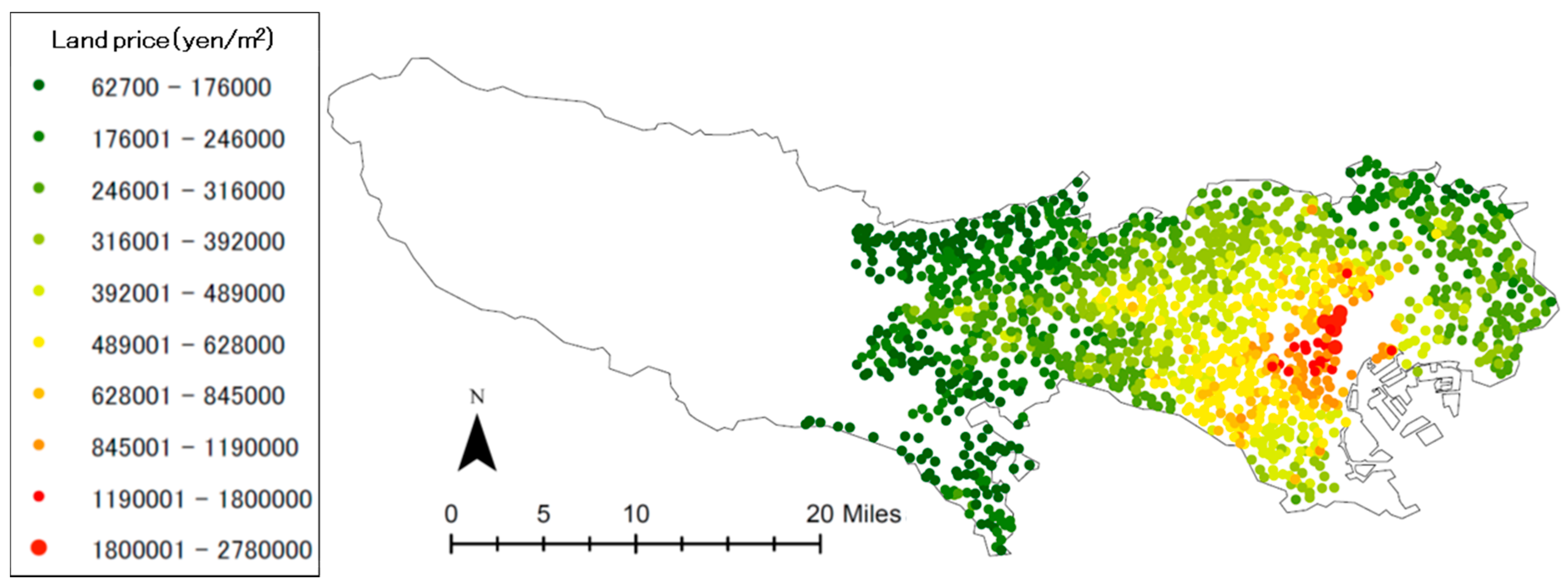
As shown in Figure 1, the distribution of residential land price in the target area in the present study was visualized using GIS, and areas with unusually high land prices were visually confirmed. From Figure 1, it is evident that land prices increase towards Tokyo station, and some residential land prices were abnormally high in Minato-ku, Chuo-ku, and Chiyoda-ku. This is because these three wards are in the city center and extremely close to the business district, which has several residential investment properties. Therefore, in order to eliminate these three wards from the target area, 1485 cases from public data of residential land price provided by the MLIT was made the target in the present study.

6. Estimations of Hedonic Price Function for Residential Area

In this section, ‘R’ will be used to confirm the multicollinearity of explanatory variables, and estimate the hedonic price function for residential areas. R is a programming language, an open-source free software for statistics analysis.

6.1. Advanced Settings for Explanatory Variables

After confirming the data using dummy variables, the results showed that “gas condition”, “water condition”, “sewage condition”, as well as “forest area/nature parks/nature conservation area” were all in the same condition in the target area. With regards to “urban planning area”, there was only one urbanization control area. For these reasons, the five dummy variables mentioned above were excluded from the explanatory variables. Additionally, “municipality division” remained the same in the target area, only with cities and wards. By means of such advanced settings for explanatory variables, 1484 cases from the public data of residential land price provided by the MLIT were chosen as targets. As there were some addresses with eight options for “direction of frontal road”, and as an error may occur when estimating the hedonic price function for residential area, data with one direction was eliminated from the explanatory variables. In addition, taking into consideration the direction most houses in Japan tend to face, it was decided that the present study would exclude “direction of frontal road (southeast)” from the explanatory variables. Based on the above,

Table 6. Explanatory Variables of the Hedonic Price Function for Residential Areas.

Explanatory Variables		Code	Overview
Quantitative variables	Distance to the closest station (m)	DS	Linear distance from the addresses taken from the public data of residential land price provided by the MLIT to the closest station
	Acreage (m2)	RA	Area of 1 residential block
	Width of Frontal road (m)	WD	Width of the road in front of the residential section
	Building coverage ratio (%)	BC	Maximum ratio of the allowed building area in the residential section
	Floor area ratio (%)	FR	Maximum ratio of the allowed gross floor area in the residential section
	Distance to Tokyo station (m)	T_DS	Linear distance from the addresses taken from the public data of residential land price provided by the MLIT to Tokyo station
	Regional vulnerability	DA	5-grade indicator of regional vulnerability for each district of each municipality
	Accessibility to destination stations	AC	A quantitative indicator that shows the convenience between the closest station to destination stations
Dummy variables (Qualitative variables)	Municipality division	C	1 for the Tama area, 0 for special wards
	Other contact surface road	A_R	1 if such areas exist, 0 if not
	Direction of frontal road (north)	N	Direction of the road in front of the residence—North
	Direction of frontal road (northeast)	NE	Direction of the road in front of the residence—Northeast
	Direction of frontal road (east)	E	Direction of the road in front of the residence—East
	Direction of frontal road (south)	S	Direction of the road in front of the residence—South
	Direction of frontal road (southwest)	SW	Direction of the road in front of the residence—Southwest
	Direction of frontal road (west)	W	Direction of the road in front of the residence—West
	Direction of frontal road (northwest)	NW	Direction of the road in front of the residence—Northwest
	Jurisdiction of frontal road	F_R	1 for private roads, 0 for public roads

lists the explanatory variables used in the present study, and

Table 7. Basic Descriptive Statistics of Data Used for Explanatory Variables.

Explanatory Variables	Mean	Median	Mode	Variance	Standard Deviation	Maximum	Minimum
PRP	376,004.25	316,000	346,000	65,162,143,940.16	255,268.77	2,780,000	62,700
DS	953.26	760	1200	481,475.53	693.88	5300	60
RA	233.05	164.5	165	98,059.71	313.14	4291	47
WD	5.93	5.4	4	11.55	3.40	40	2
BC	53.08	60	60	89.16	9.44	80	30
FR	166.37	150	200	8155.44	90.31	600	60
T_DS	17,100.42	14,162	22,672	84,863,271.86	9212.13	42,619	1574
DA	1.86	2	1	0.83	0.91	5	1
AC	79,725.99	1891.10	191,629.54	34,131,580,371.22	184,747.34	2,587,021.62	1.55 × 10−7
C	0.60	1	1	0.24	0.49	1	0
A_R	0.06	0	0	0.06	0.24	1	0
N	0.15	0	0	0.13	0.36	1	0
NE	0.08	0	0	0.07	0.27	1	0
E	0.16	0	0	0.13	0.37	1	0
S	0.17	0	0	0.14	0.38	1	0
SW	0.09	0	0	0.08	0.29	1	0
W	0.16	0	0	0.14	0.37	1	0
NW	0.08	0	0	0.08	0.28	1	0
F_R	0.09	0	0	0.08	0.29	1	0

Note PRP: Residential land price (yen/m²).

shows their basic descriptive statistics. Regarding Table 7, the number of data is 1485 as mentioned in Section 5.3.

6.2. Estimations of Hedonic Price Function for Residential Area

By applying the stepwise method as mentioned in Section 4.1, the hedonic price function for residential areas in the present study was estimated as shown in

Table 8. Estimation Results for Hedonic Price Function for Residential Area (1484 cases).

Explanatory Variables		When Using All Explanatory Variables				When Using the Sequential Selection Method
		Factor	t Value	p Value		Factor	t Value	p Value
Constant terms		9.73 × 105	21.16	<2.00 × 10−16	***	9.68 × 105	22.207	<2.00 × 10−16	***
Quantitative variables	DS	−5.86 × 10	−8.505	<2.00 × 10−16	***	−5.85 × 10	−8.502	<2.00 × 10−16	***
	RA	1.28 × 102	8.227	4.19 × 10−16	***	1.33 × 102	9.048	<2.00 × 10−16	***
	WD	3.58 × 103	2.448	1.45 × 10−2	*	3.93 × 103	2.728	6.44 × 10−3	**
	BC	−3.49 × 103	−4.086	4.62 × 10−5	***	−3.49 × 103	−4.099	4.38 × 10−5	***
	FR	5.57 × 102	6.11	1.27 × 10−9	***	5.73 × 102	6.345	2.96 × 10−10	***
	T_DS	−1.88 × 10	−17.805	<2.00 × 10−16	***	−1.87 × 10	−17.737	<2.00 × 10−16	***
	DA	−8.70 × 104	−14.88	<2.00 × 10−16	***	−8.68 × 104	−14.862	<2.00 × 10−16	***
	AC	2.01 × 10−1	8.864	<2.00 × 10−16	***	2.02 × 10−1	8.962	<2.00 × 10−16	***
Dummy variables	C	−3.52 × 104	−1.897	5.80 × 10−2	*	−3.33 × 104	−1.81	7.05 × 10−2	*
	A_R	1.90 × 104	0.952	3.41 × 10−1
	N	−6.40 × 103	−0.37	7.11 × 10−1
	NE	2.31 × 103	0.114	9.09 × 10−1
	E	−1.69 × 104	−0.982	3.26 × 10−1		−2.29 × 104	−1.898	5.79 × 10−2	*
	S	−1.53 × 104	−0.903	3.67 × 10−1		−2.12 × 104	−1.82	6.90 × 10−2	*
	SW	1.92 × 104	0.993	3.21 × 10−1
	W	−4.48 × 104	−2.627	8.70 × 10−3	**	−5.14 × 104	−4.313	1.72 × 10−5	***
	NW	2.61 × 104	1.09	2.76 × 10−1
	F_R	−1.80 × 104	−1.204	2.29 × 10−1
Adjusted R2		0.6044				0.6043

Note: *** indicates significance at 0.1% level, ** at 1% level, and * at 5% level.

. It is evident that 60% of residential land prices in the target area can be expressed using Equation (4):

$$\begin{array}{ll}\mathrm{PRP}=9.68\times {10}^5& -5.85\times 10\mathrm{DS}+1.33\times {10}^2\mathrm{RA}+3.93\times {10}^3\mathrm{WD}\\ & -3.49\times {10}^3\mathrm{BC}+5.73\times {10}^2\mathrm{FR}-1.87\times 10\mathrm{T}\_\mathrm{DS}\\ & -8.68\times {10}^4\mathrm{DA}+2.02\times {10}^{-1}\mathrm{AC}-3.33\times {10}^4\mathrm{C}-2.29\times {10}^4\mathrm{E}\\ & -2.12\times {10}^4\mathrm{S}-5.14\times {10}^4\mathrm{W}\end{array}$$

(4)

• PRP: Residential land price (yen/m²).
• DS: Distance to the closest station (m).
• RA: Acreage (m²).
• WD: Width of the road in front of the residential section (m).
• BC: Building coverage ratio (%).
• FR: Floor area ratio (%).
• T_DS: Distance to Tokyo station (m).
• DA: Regional vulnerability.
• AC: Accessibility to destination stations.
• C: Municipality division.
• E: Direction of frontal road (east).
• S: Direction of frontal road (south).
• W: Direction of frontal road (west).

6.3. Determining the Multicollinearity of Explanatory Variables

The multicollinearity of explanatory variables is determined in this section. In multiple regression analysis, as the prediction model is made up of a combination of 1 objective variable with 2 or more explanatory variables, each explanatory variable must be independent. However, as land prices are a result of many contributing factors, some attributes may be correlated. Appropriate predictions may be difficult, if explanatory variables have a significantly strong correlation. Such an issue is called the multicollinearity issue.

Variance Inflation Factor (VIF) is used to determine multicollinearity. Generally, VIF is preferably 2 or less; it is a multicollinearity issue if the results are 10 or over (Uchida 2011). The present study focuses on this point, and determines whether the VIF of each explanatory variable was 10 or under, after estimating the hedonic price function for residential areas.

Table 9. List of VIF of Explanatory Variables.

Explanatory Variables	When Using All Explanatory Variables	When Using the Sequential Selection Method
DS	1.32	1.31
RA	1.36	1.22
WD	1.42	1.38
BC	3.75	3.73
FR	3.89	3.83
T_DS	5.43	5.41
DA	1.63	1.62
AC	1.08	1.07
C	4.77	4.69
A_R	1.27
N	2.26
NE	1.67
E	2.27	1.12
S	2.36	1.12
SW	1.79
W	2.30	1.12
NW	1.73
F_R	1.09

lists the VIF of each explanatory variable. The VIF of each explanatory variable was under 10 indicating that there is no problem of multicollinearity.

7. Evaluation of Hedonic Price Function for Residential Area

7.1. Estimation of Hedonic Price Function for Residential Area Using Conventional Explanatory Variables

‘Regional vulnerability’ and ‘accessibility to destination stations’ were excluded from explanatory variables, and in the same process as described in Section 6, hedonic price function for residential area was estimated as shown in

Table 10. Estimation Results of Hedonic Price Function for Residential Area Using Conventional Explanatory Variables (1484 cases).

Explanatory Variables		When Using All Explanatory Variables				When Using the Sequential Selection Method
		Factor	t Value	p Value		Factor	t Value	p Value
Constant terms		9.12 × 105	18.224	<2.00 × 10−16	***	9.13 × 105	19.182	<2.00 × 10−16	***
Quantitative variables	DS	−5.31 × 10	−7.021	3.35 × 10−12	***	−5.33 × 10	−7.066	2.45 × 10−12	***
	RA	1.76 × 102	10.526	<2.00 × 10−16	***	1.83 × 102	11.548	<2.00 × 10−16	***
	WD	4.95 × 103	3.085	2.07 × 10−3	**	5.33 × 103	3.37	7.71 × 10−4	***
	BC	5.42 × 103	−5.829	6.86 × 10−9	***	−5.42 × 103	−5.848	6.12 × 10−9	***
	FR	5.97 × 102	5.972	2.94 × 10−9	***	6.10 × 102	6.143	1.04 × 10−9	***
	T_DS	1.77 × 10	−15.471	<2.00 × 10−16	***	−1.76 × 10	−15.436	<2.00 × 10−16	***
Dummy variables	C	7.88 × 104	−3.892	1.04 × 10−4	***	−7.66 × 104	−3.815	1.42 × 10−4	***
	A_R	2.71 × 104	1.237	2.16 × 10−1
	N	−1.68 × 104	−0.884	3.77 × 10−1		−2.51 × 104	−1.78	7.54 × 10−2	*
	NE	1.61 × 103	0.072	9.42 × 10−1
	E	−2.87 × 104	−1.52	1.29 × 10−1		−3.69 × 104	−2.645	8.25 × 10−3	**
	S	−2.59 × 104	−1.392	1.64 × 10−1		−3.46 × 104	−2.558	1.06 × 10−2	*
	SW	1.76 × 104	0.828	4.08 × 10−1
	W	−6.12 × 104	−3.266	1.12 × 10−3	**	−7.03 × 104	−5.085	4.14 × 10−7	***
	NW	1.24 × 104	0.569	5.69 × 10−1
	F_R	−1.15 × 104	−0.701	4.83 × 10−1
Adjusted R2	0.5200					0.5207

Note: *** indicates significance at 0.1% level, ** at 1% level, and * at 5% level.

. Around 52% of residential land prices in the target area using only conventional explanatory variables can be expressed using Equation (5):

$$\begin{array}{ll}\mathrm{PRP}=9.13\times {10}^5& -5.33\times 10\mathrm{DS}+1.83\times {10}^2\mathrm{RA}+5.33\times {10}^3\mathrm{WD}\\ & -5.42\times {10}^3\mathrm{BC}+6.10\times {10}^2\mathrm{FR}-1.76\times 10\mathrm{T}\_\mathrm{DS}-7.66\times {10}^4\mathrm{C}\\ & -2.51\times {10}^4\mathrm{N}-3.69\times {10}^4\mathrm{E}-3.46\times {10}^4\mathrm{S}-7.03\times {10}^4\mathrm{W}\end{array}$$

(5)

• PRP: Residential land price (yen/m²).
• DS: Distance to the closest station (m).
• RA: Acreage (m²).
• WD: Width of the road in front of the residential section (m).
• BC: Building coverage ratio (%).
• FR: Floor area ratio (%).
• T_DS: Distance to Tokyo station (m).
• C: Municipality division.
• N: Direction of frontal road (north).
• E: Direction of frontal road (east).
• S: Direction of frontal road (south).
• W: Direction of frontal road (west).

7.2. Evaluation and Examination of Hedonic Price Function for Residential Area

In this section, the hedonic price function using only conventional explanatory variables and the newly estimated hedonic price function is compared and evaluated, and the results are examined. As Table 7, Table 8 and Table 9 clearly show, there was no large difference between the results obtained using all explanatory variables and the sequential selection method.

According to the freedom-corrected determination coefficient ${\mathrm{R}}^2$, which indicates adaptability degree, the interpretability of the newly estimated hedonic price function in the present study is around 60%, while that of the hedonic price function only using conventional explanatory valuables is around 52%. As Table 8 shows, it is hard to say that the value of ${\mathrm{R}}^2$ was high. However, by adding two explanatory variables—‘regional vulnerability’ and ‘accessibility to destination stations’— that reflect residents’ reasons for selecting regions unique to Japanese metropolitan areas, the interpretability increased by 8%. Additionally, as both of these explanatory variables have a low significance level with a low p value, they are extremely important for estimating hedonic price function for residential area in Japanese metropolitan areas. Based on the characteristics of the calculation equation of accessibility to destination stations where the significance level is extremely low, regardless of the exponential changes in value, it can be said that residents place great emphasis on accessibility between the closest station and destination stations. Additionally, regarding regional vulnerability, land prices are affected by 9% if the degree of regional vulnerability changes by 1 grade as indicated in Table 8, which shows that this is another important consideration point for residents.

8. Conclusions

The estimation of hedonic price function for residential area accomplishes an important role in improving measurement of investment effects. The present study introduces and determines the usefulness of two new explanatory variables—‘regional vulnerability’ and ‘accessibility to destination stations’—that reflect the reasons for residential preferences specific to Japanese metropolitan areas. The hedonic price function in the present study was evaluated on comparison with the hedonic price function using conventional explanatory variables (with respect to significance and compatibility).

The evaluation shows that while the hedonic price function using only conventional explanatory variables had a 52% interpretability, the hedonic price function with the two new explanatory variables was greater with 60% interpretability. Additionally, it was evident that the significance level of the new explanatory variables was low, and land price changed by 9% as the regional vulnerability changed by 1 grade. Furthermore, it is also evident that residents placed great emphasis on both ‘regional vulnerability’ and ‘accessibility to destination stations’. Thus, their introduction as explanatory variables that reflect the reasons for residential preferences specific to Japanese metropolitan areas was reasonable.

However, it was confirmed that the estimation accuracy by means of hedonic price function for residential area in the present study was low in the three wards in the city center excluded from the target area; this point must be addressed. Additionally, since residential development as well as maintenance of the railway transportation system are simultaneously implemented in Japanese metropolitan areas, it is necessary to consider explanatory variables that reflect the differences in train lines. Furthermore, Kanda and Isoda (2017) proposed a “general average distance to work” as a new explanatory variable for hedonic price function for residential area. This is based on the idea that the demand for residential properties is decided according to population density and commuting expenses. Bonetti et al. (2016) used a hedonic approach to analyze the effect of water proximity and quality on residential housing prices in the province of Milan, focusing on “spatial dependence” and using spatial regression analysis. On the other hand, it is important to try new techniques such as the regularized (penalized) regression model. Based on the points mentioned above, this is a subject for further research, especially to improve the estimation accuracy for residential land prices.

References

- Aikoh, Tetsuya, Naruko Sakiyama, and Yasushi Shoji. 2008. Analysis of Economic Effect of Green Spaces on Land Price in Residential Areas by Hedonic Approach. Landscape Research Japan 71: 727–30. [Google Scholar] [CrossRef]
- Bonetti, Federico, Stefano Corsi, Luigi Orsi, and Ivan De Noni. 2016. Canals vs. streams: To what extent do water quality and proximity affect real estate values? A hedonic approach analysis. Water 8: 577. [Google Scholar] [CrossRef]
- Bureau of Urban Development, Tokyo Metropolitan Government. 2013. District-Based Assessment of Vulnerability to Earthquake Disaster (No. 7); Tokyo: Bureau of Urban Development, Tokyo Metropolitan Government.
- Cohen, Jeffrey P., and Cletus C. Coughlin. 2008. Sptial Hedonic Models of Airport Noise, Proximity and Housing Prices. Journal of Reginal Science 48: 859–78. [Google Scholar] [CrossRef]
- Conway, Delores, Christina Q. Li, Jennifer Wolch, Christopher Kahle, and Michael Jerrett. 2010. A Spatial Autocorrelation Approach for Examining the Effects of Urban Greenspace on Residential Property Values. Journal of Real Estate Finance and Economics 41: 150–69. [Google Scholar] [CrossRef]
- Dziauddina, Mohd F., Seraphim Alvanidesb, and Neil Powec. 2013. Estimating the Effects of Light Rail Transit (LRT) System on the Property Values in the Klang Valley, Malaysia: A Hedonic House Price Approach. Jurnal Teknologi 18: 35–47. [Google Scholar] [CrossRef]
- Feng, Xia, and Brad R. Humphreys. 2016. Assessing the Economic Impact of Sports Facilities on Residential Property Values: A Spatial Hedonic Approach. Journal of Sports Economics 19: 188–210. [Google Scholar] [CrossRef]
- Fik, Timothy J., David C. Ling, and Gordon F. Mulligan. 2003. Modeling Spatial Variation in Housing Prices: A Variable Interaction Approach. Real Estate Economics 31: 623–46. [Google Scholar] [CrossRef]
- Gouriéroux, Christian, and Anne Laferrèreac. 2009. Managing hedonic housing price indexes: The French experience. Journal of Housing Economics 18: 206–13. [Google Scholar] [CrossRef]
- Hill, Robert J., and Danel Melser. 2007. Comparing House Prices across Regions and Time: A Hedonic Approach. School of Economics Discussion Paper, Sydney, NSW, Australia: University of New South Wales, 34p. [Google Scholar]
- Ismail, Suriatini. 2005. Hedonic Modelling of Housing Markets Using Geographical Information System (GIS) and Spatial Statistics: A Case Study of Glasgow, Scotland. Ph.D. thesis, University of Aberdeen, Aberdeen, UK. [Google Scholar]
- Jang, Taekyoung, Yoshitaka Aoyama, Ryoji Matsunaka, and Daisuke Kirobayashi. 2000. A Study on the Accessibility Index for Evaluating the Railway Service Level. Infrastructure Planning Review 17: 75–82. [Google Scholar] [CrossRef] [Green Version]
- Hyogo, Kanda, and Yuzuru Isoda. 2017. The Relationship between Population Density, Land Price and Commuting Flow in Metropolitan Area: The Case of Tokyo Metropolitan Area. Papers and Proceedings of the Geographic Information Systems Association 26: 1–4. [Google Scholar]
- Kim, Chong Won, Tim T. Phipps, and Luc Anselinc. 2003. Measuring the Benefits of Air Quality Improvement: A Spatial Hedonic Approach. Journal of Environmental Economics and Management 45: 24–39. [Google Scholar] [CrossRef]
- Kutsuzawa, Ryuji. 2008. Economic Analysis of Financial Market of Housing and Real Estate. Tokyo: Nippon Hyoron Sha Co., Ltd. [Google Scholar]
- Wei, Li, Kenneth Joh, Chanam Lee, Jun-Hyun Kim, Han Park, and Ayoung Woo. 2015. Assessing Benefits of Neighborhood Walkability to Single-Family Property Values: A Spatial Hedonic Study in Austin, Texas. Journal of Planning Education and Research 35: 471–88. [Google Scholar]
- Oana, Mihaescu, and Rainer vom Hofe. 2012. The Impact of Brownfields on Residential Property Values in Cincinnati, Ohio: A Spatial Hedonic Approach. Journal of Regional Analysis & Policy 42: 223–36. [Google Scholar]
- Mikanagi, Kiyoyasu, and Hisayoshi Morisugi. 1981. Social Capital and Public Investment. Tokyo: Gihodo Shuppan. [Google Scholar]
- Ministry of Internal Affairs and Communications. 2016. Survey on Time Use and Leisure Activities in 2016. Available online: http://www.stat.go.jp/data/shakai/2016/index.html (accessed on 5 July 2018).
- Ministry of Land, Infrastructure, Transport and Tourism. 2013. Public Data of Residential Land Price in 2013. Available online: http://www.land.mlit.go.jp/webland/ (accessed on 14 April 2017).
- Ministry of Land, Infrastructure, Transport and Tourism. n.d. Digital National Land Information. Available online: http://nlftp.mlit.go.jp/ksj/ (accessed on 14 April 2017).
- Mittal, Jay, and Sweta Byahut. 2017. Scenic Landscapes, Visual Accessibility and Premium Values in a Single Family Housing Market: A spatial hedonic approach. Environment and Planning B: Urban Analytics and City Science, Sage. [Google Scholar] [CrossRef]
- Nakamura, Hideo, Yoshitsugu Hayashi, and Kazuaki Miyamoto. 1981. Land Use Model in Suburban Areas. Proceedings of the Japan Society of Civil Engineers 309: 103–12. [Google Scholar] [CrossRef]
- Nomura, Koji, Miho Ohara, and Kimiro Meguro. 2009. Consideration on Change of Land Price after an Urban Earthquake–Case Study in Affected Area due to the 1995 Kobe Earthquake-. Seisan Kenkyu 61: 709–12. [Google Scholar]
- Shimuzu, Chihiro. 2004. Analysis of Real Estate Market. Tokyo: Jutaku-Shimpo-Sha Inc. [Google Scholar]
- Shimuzu, Chihiro, and Hiroshi Karawatari. 2007. Econometric Analysis of Real Estate Market. Tokyo: Asakura Publishing Co., Ltd. [Google Scholar]
- Syabri, Ibnu. 2011. The Influence of Railway Station on Residential Property Values-Spatial Hedonic Approach: The Case of Serpong’s Railway Station. Journal of Civil Engineering 18: 291–300. [Google Scholar]
- Tokuda, Masaaki. 2009. The Analysis of the Land Value by the Hedonic Approach: The Residential Quarter in Shiga Prefecture as a Subject. The Hikone Ronso 381: 183–205. [Google Scholar]
- Tse, Raymond Y. C. 2002. Estimating Neighbourhood Effects in House Prices: Towards a New Hedonic Model Approach. Urban Studies 39: 1165–80. [Google Scholar] [CrossRef]
- Uchida, Osamu. 2011. Logistic Regression Analysis Using SPSS. Tokyo: Ohmsha. [Google Scholar]
- Wanatabe, Masayuki, and Hajime Koshimizu. 2012. Effect of Line Shape’s Green to Land Price in Residential Areas. Landscape Research Japan 75: 703–6. [Google Scholar] [CrossRef]
- Winke, Tim. 2017. The impact of aircraft noise on apartment prices: A differences-in-differences hedonic approach for Frankfurt, Germany. Journal of Economic Geography 17: 1283–300. [Google Scholar] [CrossRef]
- Yahoo! n.d. JAPAN, Transit. Available online: https://transit.yahoo.co.jp/ (accessed on 14 April 2017).
- Yamaga, Hisaki, Masayuki Nakagawa, and Makoto Saito. 2002. Earthquake Risk and Land Price Formation: The case of Tokyo. Journal of Applied Regional Science 966: 1–18. [Google Scholar]
Figure 1.
Distribution of Residential Land Prices in the Target Area.