Credit Rating and Pricing: Poles Apart

Abstract

Corporate credit ratings remove the information asymmetry between lenders and borrowers to find an equilibrium price. Structured finance ratings, however, are informationally insufficient because the systematic risk of equally rated assets can vary substantially. As I demonstrate in a Monte Carlo analysis, highly-rated structured finance bonds can exhibit far higher non-linear systematic risks than lowly-rated corporate bonds. I value credit instruments under a four-moment CAPM, between and within some markets there is no one-to-one relation between expected loss (rating) and credit spread (pricing). The linear CAPM beta is insufficient, buyers and sellers need also the same information on non-linear risk to have an equilibrium.

1. Introduction

The expected loss of a credit instrument comprises an assessment of default probability as well as loss expectation in the event of a credit default. The default risk is reflected in the rating assignments of the major credit rating agencies such as Standard and Poor’s, Fitch, and Moody’s. For instance, it is Moody’s intention that the expected loss rate associated with a given rating symbol and time horizon to be the same across obligations to ensure a consistency of meaning (see Moody’s Investors Service (2009), p. 6). The same rating assigned to bond obligations issued by a nonfinancial corporation, bank, insurance, sovereign, subsovereign borrower, or a structured finance obligation must imply the same expected loss. Originally, “Moody was in effect addressing the stability of the security’s credit spread,” Moody’s Investors Service (2009) (p. 6). The idea that each rating class translates into a rating-specific credit spread can also be found in modern finance (see, e.g., Jarrow et al. (1997), Figures 5 and 6).

Ratings reduce the knowledge gap, or “information asymmetry,” between borrowers (sellers) and lenders (buyers) by providing an ordinal assessment about the expected loss. I will demonstrate that the advent of structured finance obligations and other credit derivatives has completely broken down the monotone relation between expected loss (rating) and credit spread (pricing). Even if the rating truly conveys an unbiased, powerful estimate for the expected loss of an underlying obligation,1 ratings alone are informationally insufficient for the pricing of collateralized debt obligations (CDOs) and other credit instruments.2 I will show that in equilibrium an investment-rated structured finance obligation can have a significantly higher credit spread than a subinvestment-rated corporate bond due to systematic risk. That is, rating and pricing can be far apart since there is no longer a one-to-one relation between expected loss and systematic risk for structured finance obligations.3 However, a market in which potential buyers know the true rating but cannot correctly judge the systematic risk attracts sellers offering credit derivatives of good rating quality but of low systematic risk quality which can in the end lead to a market breakdown. Thus, I will demonstrate that a necessary precondition for a credit market to have an equilibrium at all is to have symmetric information between issuers and investors on rating and systematic risk.

The beta according to the CAPM of Treynor (1962), Sharpe (1964), Lintner (1965), and Mossin (1966) based on the mean-variance criterion of Markowitz (1952) reflects the systematic risk of an asset in the form of a scaled correlation with the market.4 However, as highlighted by Embrechts et al. (1999), correlation is only a linear risk measure and of limited suitability for measuring dependence. In a stylized market, I will demonstrate that the non-linear systematic risk of credit derivatives is highly substantial and even more important than the linear CAPM beta. I thereby offer another explanation for the high expected return of highly-rated debt securities given the low CAPM beta.5

According to the criticism of Krugman (2009), financial economists rarely ask the seemingly obvious question of whether asset prices make sense given real-world fundamentals. Instead, they ask only whether asset prices make sense given other asset prices. The central insight of asset pricing is that in the absence of arbitrage there exists a risk-neutral measure $\mathbb{Q}$ equivalent to the real-world probability $\mathbb{P}$ (see Harrison and Kreps (1979)). Hence, to find the equilibrium value of any derivative you can assume a risk-neutral world without making statements about the real world. However, to be in equilibrium, market participants need first a consensus on all pricing-relevant attributes. The paper of Collin-Dufresne et al. (2012) is a case in point relevant to the pricing of CDOs. The contribution of Collin-Dufresne et al. (2012) “is to investigate the relative pricing across the stock option and CDO markets” and they provide a model “to jointly price long-dated S&P 500 options and tranche spreads on the five-year CDX index.” Summers (1985) once characterized financial economists with a parable about “ketchup economists” who “have shown that two-quart bottles of ketchup invariably sell for exactly twice as much as one-quart bottles of ketchup,” and conclude that the ketchup market is perfectly efficient. Collin-Dufresne et al. (2012) use the model of Duffie et al. (2000) in which return dynamics under the risk-neutral measure are specified and they emphasize the importance of “catastrophic” risk-neutral jumps for the pricing of highly-rated securities. Collin-Dufresne et al. (2012) remain silent on whether these “catastrophic” jumps are also a real-world phenomenon or induced by risk aversion and therefore “only” a phenomenon in the risk-neutral world.

I derive a four-moment CAPM under standard risk aversion to characterize the quality of a credit instrument by four fundamental real-world factors (i.e., three systematic risk factors in addition to the rating factor) to provide an elementary relation between risk and price. I show that aversion to fat tails primarily affects the pricing of senior debt securities whereas variance aversion has a proportionally higher impact on equity. Unlike equity, the systematic risk of senior debt is dominated by non-linear cokurtosis rather than linear covariance risk, i.e., I explain the “risk-neutral catastrophic jumps” affecting senior debt by kurtosis aversion. Instead of expressing the CAPM traditionally in terms of relative returns—which was also heavily criticized by Krugman (2009)—I express the equilibrium price in terms of the promised end-of-period face amount with the expected loss rate as a direct input. The four factors—expected loss rate, covariance, coskewness, cokurtosis—can be interpreted as quality attributes in the spirit of Akerlof (1970). In my model, the factors for each asset can simply be aggregated to obtain the corresponding factors of the portfolio.6

Finally, I will show in an empirical application that the huge losses at the trading desks of two Wall Street titans, namely Morgan Stanley and UBS, were basically realized with a CAPM beta of zero but nonetheless with considerable non-linear systematic risk. These “hedged” structured finance portfolios had no covariation with the market and were no economic assets ($\beta >0$) in the sense of Coval et al. (2009a) but unfortunately also no actuarial claims whose risk could be diversified away in large portfolios. Morgan Stanley’s and UBS’s beta-neutral structured finance portfolios were nevertheless treated as actuarial claims in the corresponding risk departments despite the portfolios’ inherent non-linear systematic risk. Even worse, they misinterpreted the small premium for non-linear systematic risk as CAPM alpha and therefore leveraged their positions. Thus, I provide empirical evidence that even “too big to fail” banks were exposed to huge risks without proper assessment about all quality attributes by considering only rating and correlation/beta.

My findings are highly relevant since structured finance markets such as the market for asset backed securities (ABSs) improve the efficiency of resource allocation and help contain systemic risk by freeing up the banks’ balance sheets. Given the absence of symmetric information, my model offers an explanation why public ABS issuances remain low in the EU as reported by the BOE and ECB (2014). The low demand for ABSs is unfortunate since “ABS can support the transmission of accommodative monetary policy in conditions where the bank lending channel may otherwise be impaired” (p. 2).

I proceed as follows: Section 2 highlights the difference between linear systematic risk (CAPM beta), non-linear systematic risk and idiosyncratic risk. In Section 3 I derive a simple four-moment equilibrium CAPM. Section 4 demonstrates that a credit market under asymmetric information about non-linear systematic risk is in a disequilibrium. Section 5 shows in an illustrative market that some credit products can have superb rating quality but also high systematic risk exposures or exactly the other way around. I also discuss the influence of counterparty risk on credit derivatives. Section 6 investigates the empirical cases of Morgan Stanley and UBS. Finally, Section 7 concludes.

2. CAPM Beta and Premium for Residual Risk

Credit portfolio distributions are typically characterized by non-linear risks such as skewness and heavy tails. However, many papers on credit portfolio risk such as Coval et al. (2009a, 2009b); Hamerle et al. (2009); Brennan et al. (2009) largely ignore the pricing of non-linear systematic risks. In their CAPM-like models, based on the credit portfolio framework of Merton (1974), an asset uncorrelated with the market portfolio $(\beta =0)$ is also assumed to be stochastically independent and therefore an actuarial claim. However, stochastic independence is too strong an assumption, the cash flows of a beta-neutral portfolio may still contain significant non-linear systematic risk which—unlike the risk of actuarial claims—cannot be diversified away in a large portfolio and must be priced. For instance, Coval et al. (2009a) resort to a kind of Black and Scholes (1973) model in discrete time in the spirit of Rubinstein (1976), but they make a crucially different assumption by changing the Gaussian assumption regarding the market portfolio:7

Proposition 1 (Black and Scholes (1973) in discrete time).

If the market portfolio M and the payoff of asset P follow a bivariate log-normal distribution such that

$$\begin{array}{cc}\hfill \left(\begin{array}{c}logM\\ logP\end{array}\right)& \sim N\left(\left(\begin{array}{c}{\mu }_M\\ {\mu }_P\end{array}\right),\left(\begin{array}{cc}{\sigma }_M^2& {\sigma }_M{\sigma }_P\rho \\ {\sigma }_M{\sigma }_P\rho & {\sigma }_P^2\end{array}\right)\right),\hfill \end{array}$$

where ρ is the correlation and if the von Neumann-Morgenstern utility function $u(·)$ of the representative agent exhibits constant relative risk aversion with risk aversion coefficient λ then the price $q_P$ of end-of-period payoff P is given by $q_p=q_{0}exp\left({\mu }_p-\lambda \rho {\sigma }_M{\sigma }_P+\frac{1}{2}{\sigma }_P^2\right)$. The Radon-Nikodym derivative $Z=M^{-\lambda }/\mathbb{E}\left[M^{-\lambda }\right]$ induces the risk-neutral measure $\mathbb{Q}$:

$$\begin{array}{cc}\hfill \left(\begin{array}{c}logM\\ logP\end{array}\right)& \stackrel{\mathbb{Q}}{\sim }N\left(\left(\begin{array}{c}{\mu }_M^{\mathbb{Q}}\\ {\mu }_P^{\mathbb{Q}}\end{array}\right),\left(\begin{array}{cc}{\sigma }_M^2& {\sigma }_M{\sigma }_P\rho \\ {\sigma }_M{\sigma }_P\rho & {\sigma }_P^2\end{array}\right)\right),\hfill \end{array}$$

where ${\mu }_P^{\mathbb{Q}}={\mu }_P-\lambda \rho {\sigma }_M{\sigma }_P=log{q}_P-log{q}_0-0.5{\sigma }_P^2$ and ${\mu }_M^{\mathbb{Q}}={\mu }_M-\lambda {\sigma }_M^2=log{q}_M-log{q}_0-0.5{\sigma }_M^2$ are the shifted means under $\mathbb{Q}$.

The proof can be found in the Appendix. By linear projection of the logarithmic portfolio cash flow $logP$ onto the logarithmic cash flow of the market portfolio $logM$, one obtains an additive, mean-square efficient decomposition into market and residual/idiosyncratic risk:

$$\begin{array}{ccc}\hfill logP-{\mu }_P^{\mathbb{Q}}& =& \beta \left(logM-{\mu }_M^{\mathbb{Q}}\right)+{\sigma }_P\sqrt{1-{\rho }^2}\nu ,\hfill \\ \hfill \frac{logP-{\mu }_P^{\mathbb{Q}}}{{\sigma }_P}& =& \rho \frac{logM-{\mu }_M^{\mathbb{Q}}}{{\sigma }_M}+\sqrt{1-{\rho }^2}\nu , \mathrm{with} \nu \sim N(0,1),\hfill \end{array}$$

(1)

with $\beta =\rho {\sigma }_P/{\sigma }_M$ denoting the CAPM beta. The inclusion of further transformations of M such as polynomial expansions cannot improve the goodness-of-fit (see Hamilton (1994), p. 102). Due to normality, the systematic risk exposure is completely described by $\beta$. That is, the residuum $\nu$ follows a standardized normal distribution under the real-world measure $\mathbb{P}$ as well as under the risk-neutral measure $\mathbb{Q}$, so there is no premium associated with this residual risk. Hence, the value of any financial derivative of P—the price ${\mathbb{E}}^{\mathbb{Q}}\left[g\left(P\right)\right]$ of any $\sigma \left(P\right)$-measurable payoff $g(·)$—can be written as:

$$\begin{array}{cc}\hfill {\mathbb{E}}^{\mathbb{Q}}\left[{\mathbb{E}}^{\mathbb{Q}}\left[\left.g\left(P\right)\right|M\right]\right]& ={\int }_{-\infty }^{\infty }{\int }_{-\infty }^{\infty }\frac{g\left(\xi \right)}{\xi {\sigma }_P\sqrt{1-{\rho }^2}}h\left(\frac{log\xi -{\mu }_P^{\mathbb{Q}}-\beta \left(logm-{\mu }_M^{\mathbb{Q}}\right)}{{\sigma }_P\sqrt{1-{\rho }^2}}\right)d\xi f^{\mathbb{Q}}\left(m\right)dm,\hfill \end{array}$$

where $f^{\mathbb{Q}}(·)$ is the probability density function (pdf) of the market factor M under the risk-neutral measure $\mathbb{Q}$, $h(·)$ is the probability density function of $\nu$ under $\mathbb{P}$ and $\mathbb{Q}$. Under the assumption of Rubinstein (1976), $f^{\mathbb{Q}}(·)$ and $h(·)$ both correspond to the Gaussian pdf $\varphi (·)$.

A common failing when giving up the Gaussian assumption is to preserve—as you will see later—the easily rejectable assumption that the residual $\nu$ is independent from M so that $\nu$ is idiosyncratic, can be diversified away and has the same distribution under $\mathbb{P}$ and $\mathbb{Q}$. Coval et al. (2009a); Brennan et al. (2009); Hamerle et al. (2009) all analyze the CDO market under assumed independence between M and $\nu$. However, under non-normality, orthogonality only implies that $\mathbb{E}\left[\nu logM\right]=\mathbb{E}\left[\nu \right]\mathbb{E}\left[logM\right]=0$ (see Hamilton (1994), p. 74). In the following, I will consider not only covariance but also coskewness and cokurtosis risk because agents under standard risk aversion care about all three co-moments. For a general credit portfolio P, I will show that $\mathbb{E}\left[\nu M^2\right]\ne 0$ and that $\mathbb{E}\left[\nu M^3\right]\ne 0$. I therefore extend the CAPM by two further statistical (co-)moments.

3. Four-Moment Valuation Model

I consider a portfolio choice problem faced by (buy-and-hold) investors/individuals in a general equilibrium involving a finite number of agents and a finite number of assets. My ultimate goal in the following sections is not to find “the best” multi-period pricing model to fit observable market prices for daily mark-to-market valuation but to show within a simple, one-period model that the non-linear systematic risk of equally rated credit products can be vastly different, and if buyers and sellers cannot agree on systematic risk then this credit market has no equilibrium. Thus, to revive the market for structured finance obligations requires a parsimonious set of publicly available systematic risk figures (such as systematic covariance, coskewness and cokurtosis)—the credit rating alone is arguably only sufficient for the market of corporate bonds.

I derive a four-moment CAPM, but not via the standard way in terms of relative returns such as Kraus and Litzenberger (1976) or Harvey and Siddique (2000), instead the equilibrium price is a function of expected loss rate and systematic risk contributions per unit notional. In other words, the risk metrics are directly measured per unit at risk. For the time being, I assume to be in a representative agent economy under standard risk aversion as defined by Kimball (1993). Later, I will extend the model for an asymmetric market. The triple $\left(\mathsf{\Omega },\mathcal{F},\mathbb{P}\right)$ is the probability space and I have a representative von Neumann-Morgenstern maximizer of expected utility whose utility function $u(·)$ exhibits the following properties:

(a)

positive marginal utility for wealth, i.e., non-satiety, or monotonicity $u^{\prime }>0$,

(b)

decreasing marginal utility for wealth, i.e., risk aversion, or concavity $u^{″}<0$,

(c)

decreasing absolute risk aversion,

(d)

decreasing absolute prudence.

The quartic utility function is compatible with non-satiation, risk aversion, decreasing absolute risk aversion, decreasing absolute prudence, with positive coefficients for odd powers and negative coefficients for even powers (see the Appendix A for a proof):

Lemma 1.

Standard risk aversion implies $u^{\prime }>0$, $u^{″}<0$, $u^{‴}>0$, and $u^{⁗}<0$.

The expected utility of a $\mathcal{F}$-measurable payoff X can be approximated by a quartic utility function via fourth-order Taylor series expanded at the point $\mathbb{E}\left[X\right]$ by assuming that the fourth moment of X and fourth derivative of $u(·)$ indeed exist (see also Samuelson (1970)):

$$\begin{array}{cc}\hfill \mathbb{E}\left[u\left(X\right)\right]\approx & u\left(\mathbb{E}\left[X\right]\right)+\frac{1}{2!}{u}^{″}\left(\mathbb{E}\left[X\right]\right)\mathbb{E}\left[{\left(X-\mathbb{E}\left[X\right]\right)}^2\right]\hfill \\ & +\frac{1}{3!}{u}^{‴}\left(\mathbb{E}\left[X\right]\right)\mathbb{E}\left[{\left(X-\mathbb{E}\left[X\right]\right)}^3\right]+\frac{1}{4!}{u}^{⁗}\left(\mathbb{E}\left[X\right]\right)\mathbb{E}\left[{\left(X-\mathbb{E}\left[X\right]\right)}^4\right].\hfill \end{array}$$

For a higher order expansion, the series converges in the case of logarithmic and power utility functions if $|X-\mathbb{E}\left[X\right]|<\mathbb{E}\left[X\right]$, $\mathbb{P}$ almost surely (see, Jurczenko and Maillet (2006), p. 81). However, even for divergent Taylor series Hlawitschka (1994) shows that truncated expansions provide “excellent approximations to expected utility for the purpose of portfolio selection” even though moments do not fulfill the axioms of coherent risk measures according to Artzner et al. (1999).

Lemma 2.

A quartic von Neumann-Morgenstern utility $u(·)$ exhibiting standard risk aversion implies preference for right-skewness and preference for platykurtic distributions.

Similar as in Brennan (1979), I derive the equilibrium prices in a one-period, one-good economy with a capital market with $K+1$ assets with end-of-period payoffs $\left\{Y_0,\dots ,Y_K\right\}$ as though there existed only identical representative agents, i.a., all N buy-and-hold investors have the same probability beliefs and the same utility function. The payoff $Y_0$ is assumed to be strictly positive and non-random.

Proposition 2 (Symmetric equilibrium).

Today’s equilibrium price $q_k$ of payoff $Y_k$ at the end of the period for any $k\in \left\{1,\dots ,K\right\}$ can be expressed in terms of risk-free asset 0:

$$\begin{array}{cc}\hfill \frac{q_k}{q_0}& =\mathbb{E}\left[\frac{u^{\prime }\left(w\right)}{\mathbb{E}\left[u^{\prime }\left(w\right)\right]}\frac{Y_k}{Y_0}\right]=\mathbb{E}\left[Z\frac{Y_k}{Y_0}\right]={\mathbb{E}}^{\mathbb{Q}}\left[\frac{Y_k}{Y_0}\right],\hfill \end{array}$$

(2)

where the variable $Z=u^{\prime }\left(w\right)/\mathbb{E}\left[u^{\prime }\left(w\right)\right]$ has mean one and is positive under the assumption of non-satiation, i.e., $u^{\prime }>0$, Z therefore fulfills all requirements of a Radon-Nikodym derivative. The Radon-Nikodym derivative Z induces a measure change from the real-world measure $\mathbb{P}$ to the risk-neutral measure $\mathbb{Q}$, i.e.,

$$\begin{array}{c}\hfill \mathbb{Q}\left\{A\right\}=\mathbb{E}\left[{\mathbf{1}}_{A}Z\right],\end{array}$$

(3)

where ${\mathbf{1}}_A$ is the indicator function of any event $A\in \mathcal{F}$.8

The proof can be found in the Appendix. Without loss of any generality, I assume that the price of the risk-less asset $q_0$ is expressed per unit notional, i.e., $q_0\mapsto q_0/Y_0$, to approximate the equilibrium relation in (3) with the first four statistical moments and first four mathematical derivatives of $u(·)$:

Proposition 3 (4-moment CAPM).

Under the assumption of a representative von Neumann-Morgenstern expectation maximizers under standard risk aversion whose utility function $u(·)$ is approximated by a fourth order Taylor series around the mean end-of-period wealth w, today’s equilibrium price $q_X$ under the pricing measure $\mathbb{Q}$ in (3) of any $\mathcal{F}$-measurable financial derivative payoff X can be written as follows:

$$\begin{array}{cc}\hfill \frac{q_X}{q_0}& ={\mu }_X-{\lambda }^{\beta }{\beta }_X-{\lambda }^{\gamma }{\gamma }_X-{\lambda }^{\delta }{\delta }_X,\hfill \end{array}$$

(4)

with ${\mu }_X=\mathbb{E}\left[X\right]$, and

$$\begin{array}{cc}\hfill {\beta }_X& =\frac{\mathbb{E}\left[\left(X-\mathbb{E}\left[X\right]\right)\left(M-\mathbb{E}\left[M\right]\right)\right]}{\mathbb{E}\left[{\left(M-\mathbb{E}\left[M\right]\right)}^2\right]}\hfill \\ \hfill {\gamma }_X& =\frac{\mathbb{E}\left[\left(X-\mathbb{E}\left[X\right]\right){\left(M-\mathbb{E}\left[M\right]\right)}^2\right]}{\mathbb{E}\left[{\left(M-\mathbb{E}\left[M\right]\right)}^3\right]}\hfill \\ \hfill {\delta }_X& =\frac{\mathbb{E}\left[\left(X-\mathbb{E}\left[X\right]\right){\left(M-\mathbb{E}\left[M\right]\right)}^3\right]}{\mathbb{E}\left[{\left(M-\mathbb{E}\left[M\right]\right)}^4\right]},\hfill \end{array}$$

where $M=1/K{\sum }_{k=1}^K{Y}_k$ denotes the averaged payoff of the market portfolio, ${\beta }_X$ captures the covariance risk of X with M, ${\gamma }_X$ the coskewness risk, ${\delta }_X$ the cokurtosis risk. Under standard risk aversion, the premium ${\lambda }^{\gamma }$ for systematic skewness risk is positive if M is left-skewed and negative if right-skewed. The premia for variance and kurtosis risk, ${\lambda }^{\beta }$, ${\lambda }^{\delta }$, are positive.

The proof can be found in the Appendix. Note, ${\mu }_X$, ${\beta }_X$, ${\gamma }_X$, ${\delta }_X$ are computed under the physical risk measure $\mathbb{P}$ but do not depend on the degree of risk aversion or the form of the utility function $u(·)$. On the other hand, the risk premia ${\lambda }^{\beta }$, ${\lambda }^{\gamma }$, and ${\lambda }^{\delta }$ depend on $u^{\prime }$, $u^{″}$, $u^{‴}$, and $u^{⁗}$. Rating agencies provide an assessment about the expected loss ${\mu }_X$ but are silent on the other physical risk metrics ${\beta }_X$, ${\gamma }_X$, ${\delta }_X$. Two important remarks are in order: First, since the equilibrium price in (4) is not expressed in relative returns like other capital asset pricing models such as Sharpe (1964); Kraus and Litzenberger (1976); or Harvey and Siddique (2000), the risk metrics must be expressed relative to the underlying notional amount to make them comparable across instruments. Since the bond price is by convention expressed as a percentage of nominal value, for comparative statistics it is necessary to express ${\mu }_X$, ${\beta }_X$, ${\gamma }_X$, and ${\delta }_X$ of a financial derivative X also relative to its notional amount, i.e., per unit at risk.

Second, even if the relation between price and risk metrics is only approximately true in practice, the real-world risk statistics of a $\mathcal{F}$-measurable payoff X—rating ${\mu }_X$, linear systematic risk ${\beta }_X$, and non-linear systematic risk ${\gamma }_X$, ${\delta }_X$—with respect to a well-defined market portfolio (e.g., a credit default swap index like CDX or iTraxx) provide pricing-relevant information about the underlying credit quality. The absence of such publicly available risk metrics may result in a non-functioning market due to information asymmetry between buyer and seller of credit risks. The market for structured finance products may even collapse.

4. Credit Markets under Asymmetric Information

I introduce a market under asymmetric information in the spirit of Akerlof (1970). The risk metrics ${\mu }_X$, ${\beta }_X$, ${\gamma }_X$, and ${\delta }_X$ in (4) play here the role of the underlying quality of a credit derivative with payoff X. I still assume homogenous probability beliefs and risk aversions. Formally, I have the probability space $(\mathsf{\Omega },\mathcal{F},\mathbb{P})$, the sigma fields $\left\{\mathcal{B},\mathcal{S}\right\}$ and the risk-neutral measure $\mathbb{Q}$ induced by the four-moment CAPM kernel in (A8). So far, I implicitly assumed that the buyer’s information set $\mathcal{B}$ and the seller’s sigma algebra $\mathcal{S}$ are equal and both equal to the naive field $\left\{\varnothing ,\mathsf{\Omega }\right\}$. Now, the buyer still starts with the naive information $\left\{\varnothing ,\mathsf{\Omega }\right\}$, but rating agencies make public the information to calculate the mean ${\mu }_X=\mathbb{E}\left[\left.X\right|\mathcal{S}\right]$ of X under the seller’s information $\mathcal{S}\supset \left\{\varnothing ,\mathsf{\Omega }\right\}$ so that a potential buyer has then the sigma algebra generated by ${\mu }_X$ available for decision making, i.e., $\mathcal{B}=\sigma \left({\mu }_X\right)$.

Definition 1 (Asymmetric credit market).

In an asymmetric market, the statistical moments conditional on the seller’s information $\mathcal{S}$ and conditional on the buyer’s information $\mathcal{B}$ differ. In a symmetric market, however, the sigma algebras $\mathcal{B}$ and $\mathcal{S}$ result in the same (scaled) conditional moments ${\mu }_X$, ${\beta }_X$, ${\gamma }_X$, and ${\delta }_X$, e.g., ${\beta }_X=\mathbb{E}\left[\left.M\left(X-{\mu }_X\right)\right|\mathcal{S}\right]/\mathbb{V}\left[\left.M\right|\mathcal{S}\right]=\mathbb{E}\left[\left.M\left(X-{\mu }_X\right)\right|\mathcal{B}\right]/\mathbb{V}\left[\left.M\right|\mathcal{B}\right]$, almost surely, and I have again the equilibrium in (4). Under asymmetric information at least one of the risk metrics is different under $\mathcal{B}$ and $\mathcal{S}$.

In simple words, in an asymmetric market some pricing-relevant quality attributes are known to sellers but unknown to buyers. Such a market cannot function:

Proposition 4 (No equilibrium).

An asymmetric credit market in which sellers and buyers disagree on at least one of the four quality factors ${\mu }_X$, ${\beta }_X$, ${\gamma }_X$, ${\delta }_X$ has no equilibrium.

Proof. 

To show that a market with such asymmetric information cannot work properly, I work with a proof by contradiction, i.e., I start with the assumption that there is nonetheless an equilibrium.9 By $p_X$ I denote the compounded equilibrium price $q_X/q_0$ and by $r_X$ the risk premium (credit spread) of the positive cash flow X with $\mathbb{P}\left\{X=0\right\}<1$. The positivity assumption is without loss of generality because a payoff with negative outcomes can be split into a long and short position of two positive cash flows. Thus, the price of X is given by:

$$\begin{array}{c}\hfill p_X={\mu }_X-r_X \mathrm{where} p_X=q_X/q_0 \mathrm{and} r_X=f\left({\beta }_X,{\gamma }_X,{\delta }_X\right).\end{array}$$

(5)

From Proposition 3, I know that $p_X$ is indeed the equilibrium price under symmetric information and a four-moment CAPM when ${\beta }_X$, ${\gamma }_X$, ${\delta }_X$ are known. However, now I assume that ${\mu }_X$ is known but at least one of the factors ${\beta }_X$, ${\gamma }_X$, ${\delta }_X$ is only known to the seller ($\mathcal{S}$-measurable) but not known to the buyer (not $\mathcal{B}$-measurable). In particular, I assume there is no $\mathcal{B}$-measurable pricing function $g(·)$ such that $g\left({\mu }_X\right)=p_X$, but the buyer knows that

$$\begin{array}{c}\hfill r_X\le {\mu }_X.\end{array}$$

(6)

The upper bound in (6) must be ${\mu }_X$, otherwise an arbitrage opportunity would arise for a positive end-of-period payoff X must have a positive price with probability one. Now, conditional on the information generated by ${\mathbf{1}}_{\left\{r_X\ge {\mu }_X-p_X\right\}}$ and ${\mu }_X$, the buyer of payoff X knows that the mean risk premium on offer at the assumed equilibrium price $p_X$ is given by:

$$\begin{array}{c}\hfill {\overline{r}}_X:={\mathbb{E}}^{\mathbb{Q}}\left[r_X\left|{\mathbf{1}}_{\left\{r_X\ge {\mu }_X-p_X\right\}},{\mu }_X\right.\right].\end{array}$$

The expectation is taken under the risk-neutral measure $\mathbb{Q}$ induced by the Radon-Nikodym derivative in (A8) to account for risk aversion. The price bidden $p_X^{\ast }$ by the buyer given she knows ${\mu }_X$ and that the average risk premium on offer is ${\overline{r}}_X$ is therefore given by:

$$\begin{array}{c}\hfill p_X^{\ast }={\mu }_X-{\mathbb{E}}^{\mathbb{Q}}\left[r_X\left|{\mathbf{1}}_{\left\{r_X\ge {\overline{r}}_X\right\}},{\mu }_X\right.\right].\end{array}$$

(7)

Since

$$\begin{array}{ccc}\hfill {\overline{r}}_X={\mathbb{E}}^{\mathbb{Q}}\left[r_X\left|{\mathbf{1}}_{\left\{r_X\ge {\mu }_X-p_X\right\}}\right.,{\mu }_X\right]\le {\mathbb{E}}^{\mathbb{Q}}\left[r_X\left|{\mathbf{1}}_{\left\{r_X\ge {\overline{r}}_X\right\}},{\mu }_X\right.\right]& \iff & p_X^{\ast }\le p_X.\hfill \end{array}$$

However, the bid price $p_X^{\ast }$ is always smaller than the assumed equilibrium price $p_X$. I only have a strict equality if $p_X=0$ or else if $r_X$ is $\sigma \left({\mu }_X\right)$-measurable so that ${\overline{r}}_X=r_X$. However, a positive end-of-period cash flow X with $\mathbb{P}\left\{X=0\right\}<1$ must have a strictly positive price to exclude arbitrage and if $r_X$ is a function of ${\mu }_X$ then the market is symmetric, i.e., the rating is sufficient for pricing. I have a contradiction that $p_X$ is the equilibrium price under asymmetric information. That is, there is no equilibrium price $p_X$ and therefore no risk-neutral risk measure $\mathbb{Q}$. No trade takes place. ☐

Note, the rating can be sufficient for pricing in a four-moment CAPM. Technically speaking, in this special case, the factors ${\beta }_X,{\gamma }_X,{\delta }_X$ in (5) are $\sigma \left({\mu }_X\right)$-measurable and the rating is informationally sufficient in order to have an equilibrium. Sufficiency may hold for the segment of corporate bonds, but in general there is no rating-pricing nexus. On the contrary, as I will show, the risk premium can even be negative for derivatives with high expected losses and significantly positive for structured finance obligations of high rating quality. Counterparty risk further complicates the quality assessment of financial derivatives. As a consequence, besides the expected payoff ${\mu }_X=\mathbb{E}\left[\left.X\right|\mathcal{S}\right]$ as quality factor of a financial derivative X, I suggest making also public the systematic risk as the contribution to the variance with respect to a well-diversified portfolio M, ${\beta }_X=\mathbb{E}\left[\left.X\left(M-{\mu }_M\right)\right|\mathcal{S}\right]/\mathbb{V}\left[\left.M\right|\mathcal{S}\right]$, as well as the contribution to third moment ${\gamma }_X$, and contribution to fourth moment ${\delta }_X$ (again under the seller’s information set $\mathcal{S}$) so that $\mathcal{B}=\sigma \left({\mu }_X,{\beta }_X,{\gamma }_X,{\delta }_X\right)$ for the smooth functioning of markets. Importantly, the information to calculate the risk figures must be made public, not necessarily the factors themselves. Thus, ordinal assessments can be sufficient.

5. Results and Discussion in a Stylized Market

Coval et al. (2009a), Brennan et al. (2009), Blöchlinger (2011) have already concluded that, given the same credit rating, structured asset backed securities should offer a higher risk premium than single-name corporate bonds (except for the most senior tranche, see Blöchlinger (2018)). Surprisingly, this implication turns out not to be supported by the data. In the following, I will show in a controlled Monte Carlo experiment that structuring credit derivatives can inherently create significant systematic risks. I thereby control the credit rating: Given the same expected loss rate, the (non-linear) systematic risk can vary massively across credit instruments.

Thus, to demonstrate the often non-monotone relation between rating and systematic risk of various credit instruments, I create a stylized market with underlying digital bonds, i.e., bonds which can be synthetically replicated by digital default swaps.

Assumption 1.

I have the following market:

(1) 

The market portfolio $\left\{Y_1,\dots ,Y_K\right\}$ consists of $K=1000$ default-risky digital bonds. Each bond pays out one (notional amount) in case of survival and zero else. The price $q_0$ of the risk-free bond with end-of-period payoff $Y_0=1$, almost surely, is one.

(2) 

The binary payoff $Y_k$ for any $k\in \left\{1,\dots ,K\right\}$ is driven by two independent standardized Gaussian factors, namely a systematic factor m and an idiosyncratic factor ${ϵ}_k$:

$$\begin{array}{c}\hfill Y_k={\mathbf{1}}_{\left\{\sqrt{\rho }m+\sqrt{1-\rho }{ϵ}_k\le D{D}_k\right\}},\end{array}$$

where ${\mathbf{1}}_{\left\{·\right\}}$ is the indicator function and $D{D}_k$ is the distance to default. The sequence of idiosyncratic factors $\left\{{ϵ}_1,\dots ,{ϵ}_K\right\}$ is independent and identically distributed.

(3) 

I have four equally sized groups of 250 digital bonds with unconditional default probabilities (PDs) of 0.1%, 0.3%, 0.9%, and 2.7% such that $D{D}_1,\dots ,D{D}_{250}=3.09$, $D{D}_{251},\dots ,D{D}_{500}=2.75$, $D{D}_{501},\dots ,D{D}_{751}=2.37$, and $D{D}_{751},\dots ,D{D}_K=1.93$.

(4) 

The correlation coefficient ρ to induce default dependence equals $12\%$.

Note, the real-world correlation $\rho$ under $\mathbb{P}$ should not be confused with the asset correlation in the risk-neutral world under $\mathbb{Q}$ as used by Hull and White (2004); Li and Zhao (2012); Andersen et al. (2003); O’Kane and Livesey (2004) for pricing. My parametrization of $\rho$ in the real world is motivated by Blöchlinger and Leippold (2011), Blöchlinger (2012). The correlation $\rho$ controls, i.a., variance, skewness and kurtosis of the market portfolio M under the physical measure $\mathbb{P}$. Because I am in a one-period CAPM economy, $\rho$ is by definition fixed and neither stochastic nor a time/maturity-dependent function (=correlation curve) as in a multi-period mark-to-market valuation model. Under my set of assumptions, the end-of-period cash flow of the market portfolio can be written as:

$$\begin{array}{c}\hfill M=\frac{1}{K}\sum _{k=1}^K{Y}_k=\frac{1}{K}\sum _{k=1}^K{\mathbf{1}}_{\left\{\sqrt{\rho }m+\sqrt{1-\rho }{ϵ}_k\le D{D}_k\right\}}.\end{array}$$

The higher the distance to default $D{D}_k$, the lower is the kth bond’s physical default probability, and the mean payoff ${\mu }_k$ of bond k can be written as:

$$\begin{array}{c}\hfill {\mu }_k={\int }_{-\infty }^{\infty }\mathsf{\Phi }\left(\frac{D{D}_k-\sqrt{\rho }m}{\sqrt{1-\rho }}\right)\varphi \left(m\right)dm=\mathsf{\Phi }\left(D{D}_k\right).\end{array}$$

Note, the multivariate distribution imposed with my parametrization is the physical distribution under the real-world measure $\mathbb{P}$. The most junior tranche can be shown to be long the correlation $\rho$ while the most senior tranche is short this correlation coefficient $\rho$. However, the risk-neutral distribution under $\mathbb{Q}$ for pricing and hedging is obtained by three additional parameters in the form of the premia ${\lambda }^{\beta }$, ${\lambda }^{\gamma }$, and ${\lambda }^{\delta }$. In other words, with the correlation coefficient $\rho$ I can fit the physical pdf. Given $\rho$, with ${\lambda }^{\beta }$, ${\lambda }^{\gamma }$, ${\lambda }^{\delta }$ I can then perfectly match the risk-neutral pdf of three tranches (equity, mezzanine, senior debt). In the standard base correlation model of O’Kane and Livesey (2004), I obtain three different implied correlations to fit the prices of three different tranches.

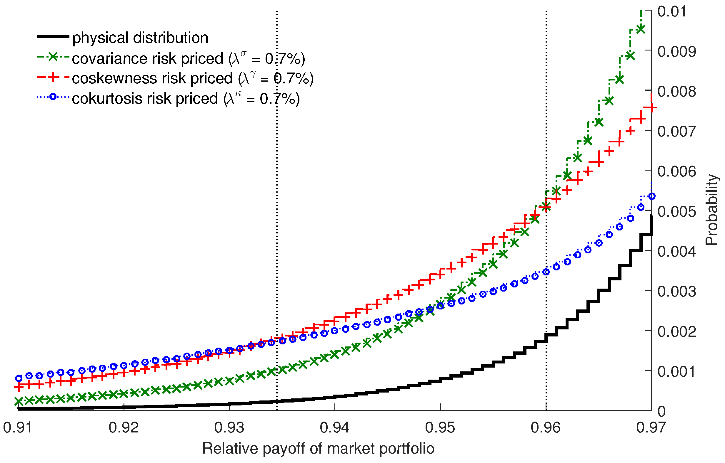
Figure 1 shows the physical and risk-neutral distributions of M. The physical distribution is skewed to the left and leptokurtic. With the cokurtosis parameter ${\lambda }^{\delta }$ I can price up and down the tail, with the standardized market price of coskewness risk ${\lambda }^{\gamma }$ I can influence in particular the middle or mezzanine part, the market premium for covariance risk ${\lambda }^{\beta }$ has the greatest effect on the first losses (equity). Figure 1 highlights the fact that for senior tranches the kurtosis contribution has a higher impact on prices than covariance (CAPM beta). Beta is particularly relevant for equity. In other words, variance aversion is more relevant for equity, kurtosis aversion more relevant for senior debt.

5.1. Single-Name Corporate Bond

The information provided by rating agencies in the form of an expected loss, i.e., the sigma algebra $\sigma ({\mu }_k)$, can be sufficient for pricing single-name bonds. The compounded price $p_k=q_k/q_0$ of a corporate bond in (5) in my illustrative market can be written as:

$$\begin{array}{c}\hfill p_k={\mu }_k-r_k=g({\mu }_k).\end{array}$$

In particular, I have the following function $g(·)$ for the compounded price $p_k$:

$$\begin{array}{c}\hfill g\left({\mu }_k\right)={\mu }_k-\sum _{j=1}^4{\mathbf{1}}_{\left\{{\mu }_k={\mu }_{1+250(j-1)}\right\}}\left\{{\beta }_{1+250(j-1)}{\lambda }^{\beta }+{\gamma }_{1+250(j-1)}{\lambda }^{\gamma }+{\delta }_{250(j-1)+1}{\lambda }^{\delta }\right\}.\end{array}$$

(8)

Simply speaking, given the corporate rating I know the credit spread and vice versa. Since ${\beta }_k$, ${\gamma }_k$, and ${\delta }_k$ are all decreasing in ${\mu }_k$ as can be seen in

Table 1. Rating and pricing of single-name digital bonds.

Digital Bond	Payoff	$\mathit{\mu }$	$\mathit{\beta }$	$\mathit{\gamma }$	$\mathit{\delta }$
AAA	$Y_0$	1.000000	–	–	–
A	$Y_1,Y_2,Y_3,\dots ,Y_{250}$	0.999000	0.1488	0.1899	0.2092
BBB	$Y_{251},Y_{252},Y_{253},\dots ,Y_{500}$	0.997000	0.3873	0.4526	0.4834
BB+	$Y_{501},Y_{502},Y_{503},\dots ,Y_{750}$	0.991000	0.9989	1.0503	1.0625
BB	$Y_{751},Y_{752},Y_{753},\dots ,Y_{1000}$	0.973000	2.4650	2.3072	2.2448
Average portfolio 1	$(Y_1+Y_{251}+Y_{501}+Y_{751})/4$	0.990000	1.0000	1.0000	1.0000
Average portfolio 2	$1/100{\sum }_{k=1}^{100}{Y}_{10(k-1)+1}$	0.990000	1.0000	1.0000	1.0000
Market portfolio	$M=1/1000{\sum }_{k=1}^{1000}{Y}_k$	0.990000	1.0000	1.0000	1.0000

There are 1000 digital bonds grouped into four subsets with default probabilities of 0.1%, 0.3%, 0.9%, and 2.7% plus one default-free bond 0. The market portfolio is the averaged payoff over all $K=1000$ digital bonds, i.e., $M=1/K{\sum }_{k=1}^K{Y}_k$. The average portfolios consist of an equal number of bonds from each group and have a variance, skewness, and kurtosis contribution of one towards the market portfolio, i.e., $\beta =\gamma =\delta =1$, the mean payoff $\mu$ of an average portfolio is 0.99. The lower the default probability of a single-name digital bond, the lower is the systematic risk. Independent from the positive risk premia there is always a monotone relation between rating ${\mu }_k$ and (compounded) price $p_k=q_k/q_0$, i.e., $p_k=g({\mu }_k)$ for any binary payoff $Y_k$, $k\in \left\{1,2,\dots ,K\right\}$. All moments and co-moments are calculated by Monte Carlo simulations with ten million draws.

, there is a monotone function $g(·)$ between rating and price, the higher the mean payoff ${\mu }_k$ the higher the price $p_k$. In general, if a credit market is homogeneous, in the sense that two bonds with the same expected loss have also the same systematic risk exposure, the information provided by rating agencies is sufficient for the market to have an equilibrium. This information symmetry between issuers and investors is no longer given for structured finance obligations.

Importantly, the risk contributions of single-name bonds in Table 1 can be used to benchmark the quality of other instruments. A AAA-rated bond has systematic risk contributions of zero. An average portfolio (consisting of an equal number of bonds from each PD class) has an expected loss of 1% and systematic risk contributions of one. Thus, a credit instrument X with risk metrics ${\beta }_X$, ${\gamma }_X$, or ${\delta }_X$ higher (lower) than one shows more (less) systematic risk exposure w.r.t. variance, skewness, or kurtosis than an average portfolio. Systematic risk contributions higher than three are worse than that of a BB-rated corporate bond.

5.2. Collateralized Debt Obligation (CDO)

To show that the relation between rating (domain) and pricing (range) is not a functional relation in case of structured asset backed securities, I create ten CDO asset pools with 100 underlying digital bonds with 25 bonds from each PD group:

$$\begin{array}{c}\hfill P_{\ell }=\frac{1}{100}\sum _{k=1}^{100}{Y}_{10(k-1)+\ell }, \mathrm{and} d_{\ell }=1-\frac{1}{100}\sum _{k=1}^{100}{Y}_{10(k-1)+\ell } \mathrm{for} \mathrm{any} \ell \in \left\{1,\dots ,10\right\},\end{array}$$

where $P_{\ell }$ is the payoff of one unit notional invested into the asset pool, $d_{\ell }=1-P_{\ell }$ denotes the default rate. I drop the index ℓ to avoid cumbersome notations in this subsection, but the index ℓ becomes relevant in a following subsection when the underlying asset pool is itself a portfolio of different CDOs (CDO squared). The jth tranche in a CDO transaction is defined by an attachment point $a_{j-1}$ and a detachment point $a_j$, such that the tranche pays out one unit if the portfolio’s default rate d is less than $a_{j-1}$, zero if it is more than $a_j$, and a linearly scaled payoff if the default rate is between $a_{j-1}$ and $a_j$. The set of attachment points is therefore given by an increasing sequence $0=a_0<a_1<\dots <a_n=1$, where n are the number of tranches. Hence, $(a_{j-1}-a_j)$ is the notional amount of tranche j. Overall, the payoff of one unit notional invested into tranche j is given by:

$$\begin{array}{ccc}\hfill T_j& =& {\mathbf{1}}_{\left\{d\le a_{j-1}\right\}}+\frac{a_j-d}{a_j-a_{j-1}}{\mathbf{1}}_{\left\{a_{j-1}<d\le a_j\right\}}.\hfill \end{array}$$

Similarly, I create seven CDO securities out of the market portfolio M with $K=1000$ underlying digital bonds. In

Table 2. Two CDO structures with 100 and 1000 underlying digital bonds.

CDO Structure 1: Asset Portfolio with 100 Underlying Digital Bonds:
$\mathit{j}$	Tranche	${\mathit{a}}_{\mathit{j}}$	Payoff	$\mathit{\mu }$	$\mathit{\beta }$	$\mathit{\gamma }$	$\mathit{\delta }$
1	First loss	0.060	$T_1={\mathbf{1}}_{\left\{d_{}\le a_0\right\}}+\frac{d_{}-a_0}{a_1-a_0}{\mathbf{1}}_{\left\{a_0<d_{}\le a_1\right\}}$	0.836149	15.2050	13.0637	11.5560
2	Mezz. $BBB-$	0.080	$T_2={\mathbf{1}}_{\left\{d_{}\le a_1\right\}}+\frac{d_{}-a_1}{a_2-a_1}{\mathbf{1}}_{\left\{a_1<d_{}\le a_2\right\}}$	0.994077	2.6560	5.5513	6.6843
3	Mezz. BBB+	0.100	$T_3={\mathbf{1}}_{\left\{d_{}\le a_2\right\}}+\frac{d_{}-a_2}{a_3-a_2}{\mathbf{1}}_{\left\{a_2<d_{}\le a_3\right\}}$	0.998245	1.0397	2.7626	3.9566
4	Senior A	0.110	$T_4={\mathbf{1}}_{\left\{d_{}\le a_3\right\}}+\frac{d_{}-a_3}{a_4-a_3}{\mathbf{1}}_{\left\{a_3<d_{}\le a_4\right\}}$	0.999299	0.5000	1.5631	2.5387
5	Senior AA	0.120	$T_5={\mathbf{1}}_{\left\{d_{}\le a_4\right\}}+\frac{d_{}-a_4}{a_5-a_4}{\mathbf{1}}_{\left\{a_4<d_{}\le a_5\right\}}$	0.999601	0.3146	1.0756	1.8789
6	Senior AAA	0.140	$T_6={\mathbf{1}}_{\left\{d_{}\le a_5\right\}}+\frac{d_{}-a_5}{a_6-a_5}{\mathbf{1}}_{\left\{a_5<d_{}\le a_6\right\}}$	0.999819	0.1614	0.6176	1.1861
7	Super senior	1.000	$T_7={\mathbf{1}}_{\left\{d_{}\le a_6\right\}}+\frac{d_{}-a_6}{a_7-a_6}{\mathbf{1}}_{\left\{a_6<d_{}\le a_7\right\}}$	0.999998	0.0026	0.0125	0.0297
Total portfolio			${\sum }_{j=1}^7\left(a_j-a_{j-1}\right)T_j$	0.990000	1.0000	1.0000	1.0000
CDO Structure 2: Asset Portfolio with 1000 Underlying Digital Bonds:
$\mathit{j}$	Tranche	${\mathit{a}}_{\mathit{j}}$	Payoff	$\mathit{\mu }$	$\mathit{\beta }$	$\mathit{\gamma }$	$\mathit{\delta }$
1	First loss	0.062	$T_1={\mathbf{1}}_{\left\{d_{}\le a_0\right\}}+\frac{d_{}-a_0}{a_1-a_0}{\mathbf{1}}_{\left\{a_0<d_{}\le a_1\right\}}$	0.839591	15.4250	13.8090	12.2459
2	Mezz. $BBB-$	0.069	$T_2={\mathbf{1}}_{\left\{d_{}\le a_1\right\}}+\frac{d_{}-a_1}{a_2-a_1}{\mathbf{1}}_{\left\{a_1<d_{}\le a_2\right\}}$	0.996991	1.9804	5.3379	7.2224
3	Mezz. BBB+	0.082	$T_3={\mathbf{1}}_{\left\{d_{}\le a_2\right\}}+\frac{d_{}-a_2}{a_3-a_2}{\mathbf{1}}_{\left\{a_2<d_{}\le a_3\right\}}$	0.998466	1.1511	3.5283	5.3279
4	Senior A	0.092	$T_4={\mathbf{1}}_{\left\{d_{}\le a_3\right\}}+\frac{d_{}-a_3}{a_4-a_3}{\mathbf{1}}_{\left\{a_3<d_{}\le a_4\right\}}$	0.999302	0.6060	2.1368	3.6412
5	Senior AA	0.100	$T_5={\mathbf{1}}_{\left\{d_{}\le a_4\right\}}+\frac{d_{}-a_4}{a_5-a_4}{\mathbf{1}}_{\left\{a_4<d_{}\le a_5\right\}}$	0.999612	0.3720	1.4431	2.6753
6	Senior AAA	0.125	$T_6={\mathbf{1}}_{\left\{d_{}\le a_5\right\}}+\frac{d_{}-a_5}{a_6-a_5}{\mathbf{1}}_{\left\{a_5<d_{}\le a_6\right\}}$	0.999847	0.1666	0.7356	1.5359
7	Super senior	1.000	$T_7={\mathbf{1}}_{\left\{d_{}\le a_6\right\}}+\frac{d_{}-a_6}{a_7-a_6}{\mathbf{1}}_{\left\{a_6<d_{}\le a_7\right\}}$	0.999999	0.0019	0.0106	0.0283
Total portfolio			$M={\sum }_{j=1}^7\left(a_j-a_{j-1}\right)T_j$	0.990000	1.0000	1.0000	1.0000

Two portfolios of 100 and 1’000 digital bonds are each structured into seven tranches, d is the default rate, $\left\{a_0,a_1,‥‥,a_7\right\}$ are attachment points. The mean payoff $\mu$ as well as the contributions $\beta$, $\gamma$, $\delta$ of the tranches of the more diversified asset pool are greater as compared to the less diversified portfolio except for the most senior tranche. Representatively weighted risk metrics over all tranches are equal since both structures represent an investment into an average bond portfolio. The most senior tranche of the more diversified asset pool is close to the risk-free bond in line with the finding of Blöchlinger (2018).

it becomes clear that there is no monotone function $g(·)$ between rating $\mu$ and price p. For instance, the sixth loss tranche with 100 underlying bonds has the lower expected payoff than the sixth loss tranche with 1000 underlying bonds, 0.999819 vs. 0.999848, but the systematic risk contributions $\beta$, $\gamma$, and $\delta$ are also lower. Depending on market prices of risks, ${\lambda }^{\beta }$, ${\lambda }^{\gamma }$, ${\lambda }^{\delta }$, the better rated security can have the lower or the higher price than the lower rated security. There is no one-to-one relation between rating and pricing as within the corporate bond segment with the function $g(·)$ in (8).

However, the credit rating is also not sufficient for pricing between bond segments: The expected payoff of the single-name digital bond with binary payoff $Y_1$ is smaller than the mean of the structured payoff $T_6$ with attachment point $a_5=0.12$ and detachment point $a_6=0.14$ as can be seen in Table 2: $0.999000=\mathbb{E}\left[Y_1\right]<\mathbb{E}\left[T_6\right]=0.999819$. So thanks to credit enhancement, investors have now an opportunity to invest into a structured security with an expected loss of 0.018% which is much better than the best rated single-name bond with an expected loss of 0.1%. However, the credit enhancement comes at a cost. The new derivative security $T_6$ shows higher covariance, coskewness, and cokurtosis with the market portfolio M than a single-name bond with a PD of 0.1%.

Especially noteworthy are two observations: First, the cokurtosis exposure of $T_6$ (under an expected loss of 0.018%) is higher than that of an average corporate bond portfolio (under a more than fifty times higher expected loss of 1%), i.e., 1.1861 vs. 1. Second, the most senior tranche of the more diversified asset pool (n = 1000 vs. n = 100) has the greater notional amount (0.875 vs. 0.86) but shows nonetheless better risks both from an expected loss and systematic exposure point of view. Thus, investing one unit into the unleveraged tranche of the more diversified asset pool with $n=$ 1000 assets is of better quality and hence has a higher price as compared to investing 10 tenth into 10 different most senior CDO tranches with 100 underlying assets. The former investment is closer to the risk-less asset 0 with ${\mu }_0=1$ and ${\beta }_0={\gamma }_0={\delta }_0=0$. This finding confirms the conclusion of Blöchlinger (2018) that the most senior tranche of a CDO transaction based on a well-diversified collateral pool can be considered a close substitute for a AAA-rated government bond. The more diversified the asset pool the better is the approximation.

It is possible to hedge the systematic risk, e.g., the following portfolio X constructed with four CDO tranches out of an underlying asset pool with 100 digital bonds in Table 2:

$$\begin{array}{c}\hfill X={\alpha }_1{T}_6-\sum _{j=2}^4{\alpha }_j{T}_j \mathrm{with} \mathrm{weights} \alpha =[3.77,0.34,-2.81,5.23],\end{array}$$

has ${\mu }_X=1$ and ${\beta }_X={\gamma }_X={\delta }_X=0$, X is still random but given my assumptions that only covariance, coskewness, and cokurtosis risk are priced, the price $q_X$ must equal the value of the (non-random) risk-free asset $q_0$. In a two-moment CAPM world, the price of all beta-neutral portfolios would be the discounted mean payoff under $\mathbb{P}$ independent from skewness or kurtosis considerations. I am going to consider now some further long-short strategies.

5.3. Long-Short Strategies of CDO Tranches

Conventional wisdom says that an asset or a portfolio of assets with a CAPM beta of zero is free of systematic risk and the remaining risk is diversifiable or idiosyncratic. After all, in the famous two-moment CAPM, the systematic risk of a security is solely measured as the contribution to the variance of the market portfolio. However, the CAPM beta is a poor statistic to measure the systematic risk exposure. Unlike conventional wisdom, the risk of a portfolio showing no correlation with the market portfolio can still be of systematic and not of diversifiable nature. To illustrate my point, I create a CDO structure with five tranches and 100 underlying digital bonds as in

Table 3. Long-short strategies with different CDO tranches.

CDO Structure with 100 Underlying Digital Bonds:
$\mathit{j}$	Tranche	${\mathit{a}}_{\mathit{j}}$	Payoff	$\mathit{\mu }$	$\mathit{\beta }$	$\mathit{\gamma }$	$\mathit{\delta }$
1	Junior	0.06	$T_1={\mathbf{1}}_{\left\{d_{}\le a_0\right\}}+\frac{d_{}-a_0}{a_1-a_0}{\mathbf{1}}_{\left\{a_0<d_{}\le a_1\right\}}$	0.836149	15.2050	13.0637	11.5560
2	Mezz. BBB	0.08	$T_2={\mathbf{1}}_{\left\{d_{}\le a_1\right\}}+\frac{d_{}-a_1}{a_2-a_1}{\mathbf{1}}_{\left\{a_1<d_{}\le a_2\right\}}$	0.994077	2.6560	5.5513	6.6843
3	Senior A	0.12	$T_3={\mathbf{1}}_{\left\{d_{}\le a_2\right\}}+\frac{d_{}-a_2}{a_3-a_2}{\mathbf{1}}_{\left\{a_2<d_{}\le a_3\right\}}$	0.998847	0.7235	2.0410	3.0827
4	Senior AAA	0.14	$T_4={\mathbf{1}}_{\left\{d_{}\le a_3\right\}}+\frac{d_{}-a_3}{a_4-a_3}{\mathbf{1}}_{\left\{a_3<d_{}\le a_4\right\}}$	0.999819	0.1614	0.6176	1.1861
5	Super Senior	1.00	$T_5={\mathbf{1}}_{\left\{d_{}\le a_4\right\}}+\frac{d_{}-a_4}{a_5-a_4}{\mathbf{1}}_{\left\{a_4<d_{}\le a_5\right\}}$	0.999998	0.0026	0.0125	0.0297
Total portfolio			${\sum }_{j=1}^5\left(a_j-a_{j-1}\right)T_j$	0.990000	1.0000	1.0000	1.0000
Long-Short Strategies with Different Tranches and One Unit Notional:
Hedge Delta			Payoff	$\mathit{\mu }$	$\mathit{\beta }$	$\mathit{\gamma }$	$\mathit{\delta }$
$\phi =0.0107$			$(1+\phi )T_4-\phi T_1$	1.001574	–	0.4841	1.0749
${\omega }_1=0.0647$			$(1+{\omega }_1)T_4-{\omega }_1{T}_2$	1.000190	–	0.2985	0.8305
${\omega }_2=0.1252$			$(1+{\omega }_2)T_4-{\omega }_2{T}_2$	1.000538	$-0.1509$	–	0.4978
${\omega }_2=0.2157$			$(1+{\omega }_3)T_4-{\omega }_3{T}_2$	1.001058	$-0.3768$	$-0.4467$	–

A beta-neutral CDO portfolio with a fourth loss tranche with payoff $T_4$ as long position can be achieved by shorting lower rated tranches. Investing $(1+\phi )$ units of notional amount in the fourth loss tranche and shorting the fraction $\phi$ of the first loss tranche results in an investment X uncorrelated with the market but with positive coskewness and above average kurtosis contribution, i.e., ${\beta }_X=0$, ${\gamma }_X>0$, ${\delta }_X>1$, so the price under the four-moment CAPM must be smaller than the discounted mean payoff ${\mu }_X$. In a two-moment CAPM, however, it would be the discounted mean. On the other hand, investing $(1+{\omega }_3)$ into the fourth loss tranche and shorting ${\omega }_3$ of the second loss tranche shows no cokurtosis with the market but both negative covariance and negative coskewness so that the four-moment CAPM price of this portfolio is greater than the discounted mean payoff.

. Starting with a long position in the fourth loss tranche with payoff $T_4$, I can create portfolios with no covariance, no coskewness, and no cokurtosis by shorting either the first or second loss tranche, i.e., shorting either $T_1$ or $T_2$.

For instance, the payoff $X=(1+\phi )T_4-\phi T_1$ with $\phi =1.07\%$ has no correlation with M, i.e., ${\beta }_X=0$, but shows significant coskewness, ${\gamma }_X=0.4841$, and cokurtosis exposure, ${\delta }_X=1.0749$. In other words, besides the CAPM beta, to understand the systematic risk of credit exposures, I need to look at skewness and kurtosis contributions, i.e., ${\gamma }_X$ and ${\delta }_X$. The market portfolio M has systematic variance, skewness, and kurtosis contributions of 1. Thus, from a systematic kurtosis perspective the leveraged portfolio X is more risky than the average bond portfolio even though X and M are not correlated. From a systematic variance point of view, however, X is as risk-less as the default-free bond.

Coval et al. (2007) create the term “economic assets,” i.e., “assets with a positive CAPM beta” (p. 7). Since X shows no covariance with the market, its beta is zero, X is no economic asset and the expected return of X must equal the risk-free return in a two-moment CAPM world. In the four-moment CAPM, however, the value of X must be lower than $q_0{\mu }_X$. On the other hand, the long-short portfolio $V=(1+{\omega }_3)T_4-{\omega }_3{T}_3$ with ${\omega }_3=21.6\%$ shows no cokurtosis with M, but negative coskewness and negative covariance with M. Under the four-moment CAPM the value of V must be higher than its discounted mean payoff, i.e., the price of V must be higher than $q_0{\mu }_V$, because V added to the market portfolio M reduces the variance and skewness of the market portfolio M, i.e., any convex combination of M and V is of better quality and therefore has a higher price than the market portfolio M alone.

5.4. CDO Squared

As CDOs developed, some dealer banks repackaged tranches into yet another iteration, known as “CDO squared” or “CDOs of CDOs”. Thus, a CDO squared is identical to a CDO except for the assets securing the obligation. Unlike the CDO, which is backed by a pool of bonds, loans and other credit instruments, CDO squared are backed by CDO tranches. CDO squared allows the banks to resell the risk that they have taken in CDOs.

Table 4. Four different CDO squared structures.

Tranche	n	Notional N	Payoff	$\mathit{\mu }$	$\mathit{\beta }$	$\mathit{\gamma }$	$\mathit{\delta }$
First loss	4	0.3750	$max\left\{\frac{P_n}{1-N}-\frac{N}{1-N},0\right\}$	0.990978	3.8883	7.6913	8.7413
Senior A			$1-max\left\{1-\frac{P_n}{N},0\right\}$	0.999219	0.6104	1.9976	3.2683
First loss	6	0.4167	$max\left\{\frac{P_n}{1-N}-\frac{N}{1-N},0\right\}$	0.990344	4.1447	8.1368	9.1597
Senior A			$1-max\left\{1-\frac{P_n}{N},0\right\}$	0.999284	0.5788	1.9427	3.2291
First loss	8	0.4375	$max\left\{\frac{P_n}{1-N}-\frac{N}{1-N},0\right\}$	0.989991	4.2868	8.3818	9.3864
Senior A			$1-max\left\{1-\frac{P_n}{N},0\right\}$	0.999311	0.5663	1.9241	3.2216
First loss	10	0.4500	$max\left\{\frac{P_n}{1-N}-\frac{N}{1-N},0\right\}$	0.989768	4.3766	8.5356	9.5273
Senior A			$1-max\left\{1-\frac{P_n}{N},0\right\}$	0.999326	0.5596	1.9146	3.2193
Underlying CDO portfolio			$P_n=\frac{1}{n}{\sum }_{\ell =1}^n{T}_{\ell 2}$	0.994077	2.6560	5.5513	6.6843

The underlying asset portfolio with payoff $P_n$ consists of n CDO mezzanine tranches. Each mezzanine tranche $T_{\ell j}$, $\ell \in \left\{1,\dots ,n\right\}$, $j=2$, has an attachment point $a_{j-1}=0.06$ and a detachment point $a_j=0.08$, and the underlying digital bond portfolio of each mezzanine tranche consists of 100 credit names. The payoff of the underlying asset portfolio $P_n$ is therefore given by:

$$P_n=\frac{1}{n}{\sum }_{\ell =1}^n{T}_{\ell j}, \mathrm{with} T_{\ell j}={\mathbf{1}}_{\left\{d_{\ell }\le a_{j-1}\right\}}+\frac{d_{\ell }-a_{j-1}}{a_j-a_{j-1}}{\mathbf{1}}_{\left\{a_{j-1}<d_{\ell }\le a_j\right\}}, d_{\ell }=1-\frac{1}{100}{\sum }_{k=1}^{100}{Y}_{10(k-1)+\ell },$$

where $Y_k$ denotes the binary payoff of digital bond k, and $d_{\ell }$ the default rate in the underlying bond portfolio of the CDO mezzanine tranche $T_{\ell j}$. The variable N denotes the notional amount of senior debt, $(1-N)$ the notional amount of equity (first loss tranche). Due to linearity, the risk contributions $\mu$, $\beta$, $\gamma$, and $\delta$ of the underlying CDO pool $P_n$ are independent from the number of underlying CDOs n. However, due to non-linear payoffs of debt and equity, the risk contributions of the CDO squared tranches depend on n (and N). The more diversified the underlying CDO pool, the higher (worse) is the quality of senior debt (equity).

shows the repackaging of second loss CDO tranches from Table 3. Each CDO squared structure consists of $n\in \left\{2,4,6,8\right\}$ underlying CDO tranches $\left\{T_{2\ell }:\ell =1,\dots ,n\right\}$ on the asset side and a senior debt tranche and an equity tranche on the liability side. The more diversified the underlying asset pool, i.e., the greater n, the higher the possible leverage N for a given rating and the systematic risk of debt (equity) decreases (increases) with increasing n. However, a CDO squared debt tranche compared to a simple CDO tranche, such as the third loss tranche in Table 3, the expected payoff $\mu$, systematic variance $\beta$, and skewness $\gamma$ are lower, but the systematic kurtosis $\delta$ is higher. In a three-moment CAPM all CDO squared debt tranches in Table 4 must have the higher price compared to the third loss tranche $T_3$ in Table 3. However, in the four-moment CAPM, the pricing relation between simple CDO and CDO squared is also influenced by $\delta$ which is higher for the latter. The CDO squared example highlights the relevance of all four quality factors for pricing risky debt.10

5.5. Credit Linked Note (CLN) under Counterparty Risk

The relation between rating and pricing can be completely turned upside down as I will demonstrate for credit linked notes (CLNs). The issuer of a CLN is not obligated to repay the notional amount in full if a specified event occurs. With the structuring of a credit linked note, I can create a payoff X with a low expected loss but high systematic risk contributions ${\beta }_X$, ${\gamma }_X$, ${\delta }_X$ or the other way around, i.e., a payoff with low rating quality but of high quality with respect to systematic risk. Besides the risk metrics of the underlying payoff characteristic X, it is the credit quality of the issuing counterparty that matters for pricing.

In

Table 5. Rating and pricing of credit linked notes under counterparty risk.

CLN	Payoff	$\mathit{\mu }$	$\mathit{\beta }$	$\mathit{\gamma }$	$\mathit{\delta }$
(1)	$0.25{\sum }_{i=1}^4{\mathbf{1}}_{\left\{Y_{1+(i-1)250}=1\right\}}{Y}_0$	0.990000	1.0000	1.0000	1.0000
(2)	${\mathbf{1}}_{\left\{1/100{\sum }_{k=1}^{100}{Y}_{(k-1)10+1}\ge 0.90\right\}}{Y}_0$	0.999296	0.5000	1.5631	2.5387
(3)	${\mathbf{1}}_{\left\{M\ge 0.91\right\}}{Y}_0$	0.999419	0.5219	1.9003	3.3286
(3a)	${\mathbf{1}}_{\left\{M\ge 0.91\right\}}{Y}_1$	0.998430	0.6582	2.0397	3.4419
(3b)	${\mathbf{1}}_{\left\{M\ge 0.91\right\}}{Y}_{251}$	0.996447	0.8825	2.2434	3.6019
(3c)	${\mathbf{1}}_{\left\{M\ge 0.91\right\}}{Y}_{501}$	0.990491	1.4593	2.7198	3.9675
(3d)	${\mathbf{1}}_{\left\{M\ge 0.91\right\}}{Y}_{751}$	0.972540	2.8610	3.7416	4.7387
(4)	${\mathbf{1}}_{\left\{M\ne 0.990\right\}}{Y}_0$	0.960958	–	1.4613	0.6652
(5)	$1-0.16\times {\mathbf{1}}_{\left\{M=0.975\right\}}-0.84\times {\mathbf{1}}_{\left\{M=0.976\right\}}$	0.992046	$-0.6652$	$-0.1250$	–
(6)	${\mathbf{1}}_{\left\{M<1.000\right\}}{Y}_0$	0.953889	$-4.3342$	$-0.1032$	$-1.0630$
(6a)	${\mathbf{1}}_{\left\{M<1.000\right\}}{Y}_1$	0.952886	$-4.1850$	0.0857	$-0.8574$
(6b)	${\mathbf{1}}_{\left\{M<1.000\right\}}{Y}_{251}$	0.950886	$-3.9445$	0.3517	$-0.5813$
(6c)	${\mathbf{1}}_{\left\{M<1.000\right\}}{Y}_{501}$	0.944896	$-3.3362$	0.9447	$-0.0073$
(6d)	${\mathbf{1}}_{\left\{M<1.000\right\}}{Y}_{751}$	0.926877	$-1.8730$	2.1965	1.1796
Market	$M=1/1000{\sum }_{k=1}^{1000}{Y}_k$	0.990000	1.0000	1.0000	1.0000

CLN (1) replicates the payoff of an average portfolio of single-name digital bonds from Table 1, CLN (2) is a binary that pays out nothing if the default rate in an average portfolio of 100 digital bonds exceeds 10%. CLN (3) pays out nothing in case the market loss exceeds 9% and one else. The credit quality decreases significantly under decreasing counterparty quality in CLN (3a), (3b), (3c) (3d). CLN (4) pays out nothing in case the market’s default rate is exactly 1% and one else, it shows no covariation with the market yet above average coskewness risk $(>1)$. CLN (5) has no cokurtosis exposure. CLN (6) pays out one but in the best state of the world when there are no market losses. Its default probability is quite high with 4.61%, but its systematic risk exposure could not be better. CLN (6a), (6b), (6c) and (6d) are the same CLN as (6) but under increasing counterparty risk. Counterparty 0 is default protected.

I create fourteen structured products. The first CLN replicates the payoff of an average bond portfolio so that the systematic risk contributions $\beta$, $\gamma$, $\delta$ are all equal to one and the expected payoff $\mu$ is 99%. CLN (2) and (3) replicate digital CDO tranches with 100 and 1000 underlying digital bonds in the asset pool. CLN (2) and (3) have far higher expected payoffs with 99.93% and 99.94% than CLN (1) with a mean payoff of 99%, but the systematic skewness and the systematic kurtosis are higher. The more diversified CLN (3) has even higher systematic risk contributions than the less diversified CLN (2). CLN (3a), (3b), (3c), (3d) take into account the issuer’s counterparty risk. In fact, CLN (3) can also be interpreted as an investment into a synthetic digital CDO tranche with the market portfolio as underlying asset pool. The systematic risk quality of such an investment is already below average regarding coskewness and cokurtosis risk $(\gamma ,\delta >1)$. However, with the inherent counterparty risk involved in a synthetic CDO, its quality factors are even worse. The “opposite” payoff of CLN 3), i.e., the payoff ${\mathbf{1}}_{\left\{M<0.91\right\}}{Y}_k$ is in effect a digital default swap (DDS) under counterparty risk k. Thus, the synthetic CDO plus DDS issued by the same counterparty k yields the payoff $Y_k$, i.e., the digital bond of issuer k. CLN (4), (5) are structured products with no systematic variance and no systematic skewness risk, respectively. CLN (4), (5) demonstrate the importance of considering non-linear systematic risk, the linear CAPM beta alone is insufficient. The price of CLN (4) entails compensation for non-linear systematic risk and not CAPM alpha. Conversely, CLN (5) is not a negative CAPM alpha investment but offers protection against systematic skewness.

CLN (6) has the lowest rating quality among instruments with no counterparty risk, i.e., it has the highest expected loss. However, CLN (6) only defaults in the best state of the economy when there are no defaults in the market portfolio, i.e., in a state when a marginal payoff is least beneficial. Apart from rating quality, CLN (6) offers the highest possible quality and is in that respect quite the opposite of CLN (3) which has the best rating quality but under quite unfavorable systematic risk. CLN (6a), 6(b), 6(c), 6(d) take into account the counterparty risk of the CLN issuer. That is, those four CLNs unlike CLN (6) can also default in bad states when the CLN issuer is not capable to fulfill its obligation. Remarkably, all four CLNs under counterparty risk still have negative betas yet their coskewness is positive, again a clear demonstration that rating and beta are insufficient for pricing.

5.6. Distress-Contingent Convertible Bond (CoCo)

My model allows the analysis of many other credit instruments such as bank deposit insurance and loan guarantees as an alternative to Merton (1977), catastrophe bonds, or credit default swaps (CDSs) under counterparty risk. However, to provide yet a final example, I will discuss distress-contingent convertible bonds or simply CoCos (see Duffie (2010)).

Let $\omega \in \left[0,1\right]$ denote the dilution factor, $\omega =0$ means that the CoCo is a pure write-down bond, existing shareholders experience no dilution at all, $\omega =1$ means that existing shareholders are wiped out completely as soon as the conversion level in the form of an attachment point $a_1$ is triggered. Such a waterfall structure can be thought of as a convolution of first, second, and third loss tranche in a standard CDO structure. The first loss is borne by the equity holder, the second loss tranche is borne by the CoCo bondholder, and claims for the third loss tranche are divided between equity and CoCo bondholder, the fraction $\omega$ belongs to the CoCo bondholder and $(1-\omega )$ to the equity holder. Consequently, by linearity the prices of equity and CoCo bond are the weighted average of a more standard CDO structure:

$$\begin{array}{cc}\mathrm{Payoff} \mathrm{equity}:\hfill & \frac{a_1{T}_1+(a_3-a_2)(1-w)T_3}{a_1+(a_3-a_2)(1-w)}\hfill \\ \mathrm{Payoff} \mathrm{contingent} \mathrm{convertible} \mathrm{bond}:\hfill & \frac{(a_2-a_1)T_2+(a_3-a_2)w{T}_3}{(a_2-a_1)+(a_3-a_2)w},\hfill \end{array}$$

where $T_1$, $T_2$, $T_3$ are the payoffs of a first, second, and third loss tranche of a standard CDO structure, $a_1$, $a_2$, $a_3$ are the attachment points. Due to linearity, the systematic risk contributions as well as the mean payoff of equity and CoCo can be obtained from the corresponding CDO tranches as listed in

Table 6. Refinancing of bank assets with equity and contingent convertible bond.

Complete Write down $\mathit{w}=0$/CoCo Bondholders Have No Claim to 3rd Loss Tranche:
Tranche	Payoff	$\mathit{\mu }$	$\mathit{\beta }$	$\mathit{\gamma }$	$\mathit{\delta }$
Equity	$\frac{a_1{T}_1+(a_3-a_2)(1-w)T_3}{a_1+(a_3-a_2)(1-w)}$	0.901228	9.4124	8.6546	8.1667
Contingent convertible bond	$\frac{(a_2-a_1)T_2+(a_3-a_2)w{T}_3}{(a_2-a_1)+(a_3-a_2)w}$	0.994077	2.6560	5.5513	6.6843
Portfolio	${\sum }_{j=1}^3\frac{a_j-a_{j-1}}{a_3-a_0}{T}_j$	0.916703	8.2864	8.1374	7.9196
Complete Dilution of Equity $\mathit{w}=1$/Equity Holders Have no Claim to 3rd Loss Tranche:
Tranche	Payoff	$\mathit{\mu }$	$\mathit{\beta }$	$\mathit{\gamma }$	$\mathit{\delta }$
Equity	$\frac{a_1{T}_1+(a_3-a_2)(1-w)T_3}{a_1+(a_3-a_2)(1-w)}$	0.836149	15.2050	13.0637	11.5560
Contingent convertible bond	$\frac{(a_2-a_1)T_2+(a_3-a_2)w{T}_3}{(a_2-a_1)+(a_3-a_2)w}$	0.997257	1.3677	3.2111	4.2832
Portfolio	${\sum }_{j=1}^3\frac{a_j-a_{j-1}}{a_3-a_0}{T}_j$	0.916703	8.2864	8.1374	7.9196

The equity holder bears the first 6% of losses (first loss tranche $T_1$ with attachment $a_0=0$ and detachment point $a_1=0.06$). The contingent convertible bondholder bears the next 2% of losses (second loss tranche $T_2$ with detachment point $a_2=0.08$), the fraction w is the payoff of the third loss tranche $T_3$ with detachment point $a_3=0.12$ that goes to the contingent convertible bondholder and $(1-w)$ to the equity holder. More senior debt holders are only affected if the losses exceed 12%. The underlying asset pool consists of 100 digital bonds. The total notional amount of contingent convertible bonds is $(a_2-a_1)+(a_3-a_2)w$, the total notional amount of equity is $a_1+(a_3-a_2)(1-w)$. As a consequence, the higher w, the lower (higher) the systematic risk exposure $\beta$, $\gamma$, $\delta$ of contingent convertible bonds (equity) per unit notional and the higher (lower) the expected payoff $\mu$.

. The higher the dilution w, the higher is the systematic risk of equity but the lower the systematic exposure of the CoCo. In other words, the lower the dilution $\omega$, the less “toxic” is equity. Under $\omega =1$, the rating quality of the CoCo is slightly better than that of a BBB-rated corporate bond in Table 1, yet its systematic skewness and kurtosis are even higher than that of a BB-rated corporate bond. Similarly, the expected loss of the CoCo is clearly lower than that of an average corporate bond portfolio, yet its systematic risk exposure is considerably worse.

6. Empirical Cases

As pointed out by Collin-Dufresne et al. (2012), “traders in the CDX market are typically thought of as being rather sophisticated. Thus, it would be surprising to find them accepting so much risk without fair compensation.” Longstaff and Rajan (2008), Li and Zhao (2012) show that CDX tranches are consistently priced under risk-neutral models and conclude that these securities are “reasonably efficiently priced.”

I provide two empirical counterexamples that even professional participants in the market for structured finance obligations, namely Morgan Stanley and UBS, were seemingly not aware of the inherent non-linear risk of apparently hedged CDO portfolios. In particular, both banks neglected the coskewness and cokurtosis risk of their trading portfolios which were basically uncorrelated with the market portfolio. Both dealer banks thought that their structured finance portfolios were of higher quality than they actually were, so I doubt whether they were really fairly compensated for their unintentional risk taking.

6.1. Morgan Stanley

According to Lewis (2011), the fixed-income trader Howie Hubler at Morgan Stanley bought insurance on BBB-rated CDOs by paying the CDS spread on a notional amount of roughly USD 2 bn. To offset his running cost he sold protection on AAA-rated CDOs by receiving the insurance fee on a notional amount of around USD 18 bn.11 In effect, Morgan Stanley synthetically constructed a leveraged structured finance portfolio with a notional N = USD 16 bn by investing $(1+1/8)N$ = USD 18 bn into AAA-rated CDO tranches and by shorting $1/8N$ = USD 2 bn of BBB tranches. As listed in Table 3, such a long-short strategy (of second- and fourth-loss tranches) is roughly beta-neutral and therefore virtually free of linear systematic risk but significantly exposed to non-linear systematic risk. From a systematic risk perspective in a two-moment CAPM, Hubler’s structure is as risk-free as Swiss or US Treasury bonds. Indeed, Hubler’s position “registered on Morgan Stanley’s internal report as virtually riskless,” Lewis (2011) (p. 207). Morgan Stanley managed to sell this leverage structure in July 2007 prior to expiration mainly to UBS with a loss of around USD 9 bn:

“The other, bigger, buyer was UBS—which took $2 billion in Howie Hubler’s triple-A CDOs, along with a couple of hundred million dollars’ worth of his short position in triple-B-rated bonds. That is, in July, moments before the market crashed, UBS looked at Howie Hubler’s trade and said, "We want some of that, too." […] traders at UBS who executed the trade were motivated mainly by their own models—which, at the moment of the trade, suggested they had turned a profit of $30 million.”

Lewis (2011) (p. 215/216)

In the first half of 2007, buyers of CDOs were gradually realizing that there are unknown quality factors in the sense of Akerlof (1970). UBS was arguably the last buyer before the market broke down completely: “In the second quarter of 2007 […] The UBS leadership continued to be optimistic and the Investment Bank went on purchasing highly rated subprime paper while other banks were quickly unloading their positions” Straumann (2010).

6.2. UBS

UBS incentivized its business divisions with an UBS-specific economic value added approach of Ospel-Bodmer (2001) which is fundamentally based on a two-moment CAPM. In the framework of Ospel-Bodmer (2001) there is no mentioning of non-linear risk, there is just an alpha and a CAPM beta, so the compensation for non-linear systematic risk is falsely interpreted as economic value added, economic profit, or CAPM alpha.

As seen above, UBS took over some CDO risks from Morgan Stanley by buying a beta-neutral long-short CDO portfolio. The conventional thinking that only beta measures systematic risk seems to have been deeply ingrained at UBS that ultimately reported net losses of 18.7 bn. In its shareholder report, UBS (2008) called its long-short CDO portfolio “Amplified Mortgage Portfolio” Super Seniors (AMPS): “these were Super Senior positions where the risk of loss was initially hedged through the purchase of protection on a proportion of the nominal position (typically between 2% and 4% though sometimes more)” (p. 14).12 That is, UBS was long senior CDO tranches and hedged its position by shorting first or second loss CDO tranches. These long-short strategies are roughly beta-neutral as can be seen in Table 3 and explain the majority of losses at UBS (2008): “As at the end of 2007, losses on these AMPS trades contributed approximately 63% of total Super Senior losses” (p. 14).

However, even with the benefit of hindsight, UBS seems to have misunderstood the principal root cause of their losses. UBS (2008) states that its losses were primarily of idiosyncratic and not of systematic nature: “Trading losses: Insufficient accounting for the risk of divergent movements between previously correlated asset classes or instruments (basis risk)” and “insufficient attention to idiosyncratic risk factors (i.e., the risk of price change due to unique circumstances of a specific security, as opposed to the overall market)” (p. 30). The fact that the remaining risk was systematic and not idiosyncratic should have been obvious because a full hedge by insurance via CDS on the exactly same underlying (in UBS vocabulary a NegBasis trade), was more costly than beta-neutral hedging (AMPS trade).13 If the remaining risk of a beta-neutral portfolio were indeed purely idiosyncratic there would have been no risk premium: “The cost of hedging through a NegBasis was approximately 11 bp, whereas the cost of hedging through an AMPS trade was approximately 5–6 bp. The reasons for the differential pricing of hedging strategies that from a risk metrics perspective were deemed equivalent appears not to have been closely scrutinised,” UBS (2008) (p. 30).

In other words, the cost of full protection against systematic risk was around 0.10%, roughly half of the premium was for linear systematic risk and the other half for non-linear systematic risk. However, with their beta-neutral AMPS portfolio, UBS paid only around 0.05% for protection against linear systematic risk and left the non-linear systematic risk unhedged. Already an increase in the market price of kurtosis risk later resulted in a significant mark-to-market loss. Nonetheless, UBS (2008) considered its positions as completely hedged: “Once hedged, either through NegBasis or AMPS trades, the Super Senior positions were VaR and Stress Testing neutral (i.e., because they were treated as fully hedged, the Super Senior positions were netted to zero and therefore did not utilize VaR and Stress limits)” (p. 30).14 Given UBS’s ignorance of non-linear systematic risk, UBS was hardly fairly compensated and it is not surprising that UBS was considered “the biggest fool at the table” (p. 215) according to Lewis (2011).15

7. Conclusions

I offer an explanation in the spirit of Akerlof (1970) for the fall of the structured credit market after the financial market crisis in 2007/08 and why we still see problems resuscitating this market (see, e.g., Segoviano et al. (2015)). The systematic risk of two credit instruments with the same rating can vary substantially, in particular the non-linear systematic risk, but the systematic risk—unlike the rating—is not readily available to the average investor. That is, structured credit ratings are informationally insufficient for pricing even if ratings provide unbiased, powerful estimates on expected losses. However, a market in which potential buyers cannot correctly assess all pricing-relevant attributes of a product can attract sellers offering inferior goods, in particular, credit products of good rating quality but low systematic risk quality. The presence of market participants who are willing to offer inferior goods tends to drive the market out of existence.

I propose to assess the quality of a credit instrument with end-of-period payoff X by four statistical (co-)moments: mean ${\mu }_X$, covariance ${\beta }_X$, coskewness ${\gamma }_X$, cokurtosis ${\delta }_X$, where the three latter metrics are expressed with respect to a well-diversified portfolio M. Currently, rating agencies offer an assessment only about ${\mu }_X$ but are silent about ${\beta }_X$, ${\gamma }_X$, ${\delta }_X$. In other words, besides the rating information to compute the expected payoff ${\mu }_X=\mathbb{E}\left[\left.X\right|\mathcal{S}\right]$ under the issuer’s information $\mathcal{S}$, I suggest making also public the systematic risk, i.e., the contribution of X to the variance of M as well as the contributions to the third and fourth central moment of M (always conditional on the seller’s information $\mathcal{S}$). I show that a market in which potential buyers are ignorant about at least one of the four quality attributes has no equilibrium. Making public the seller’s information about ${\mu }_X$, ${\beta }_X$, ${\gamma }_X$, ${\delta }_X$, not only ${\mu }_X$, results in a symmetric market with an equilibrium. Such holistic quality assessments for more complex credit instruments can then be benchmarked against simple single-name bonds. As I illustrate, an investment-rated structured finance obligation can have worse systematic risk qualities than a subinvestment-rated corporate bond.

With additional assumptions (i.a., the well-diversified portfolio M is the market portfolio), I offer a simple and straightforward four-moment CAPM that combines the quality attributes of a credit instrument ${\mu }_X$, ${\beta }_X$, ${\gamma }_X$, and ${\delta }_X$ into an equilibrium price $g({\mu }_X,{\beta }_X,{\gamma }_X,{\delta }_X)$. The variables ${\mu }_X$, ${\beta }_X$, ${\gamma }_X$, and ${\delta }_X$ are real-world risk metrics independent from any preference assumptions. To arrive at the pricing function $g(·)$, I assume having a representative agent under standard risk aversion, inter alia.

The fact that single-name bonds, structured finance securities and other credit products carry systematic risk contributions $\beta$, $\gamma$, $\delta$ that can be so different from a pricing standpoint casts significant doubt on whether some credit markets can really smoothly function with only the information provided by rating agencies about the expected payoff $\mu$. The corporate bond market is possibly homogenous enough but other credit markets—in particular CDOs—certainly not. I illustrate that systematic risk cannot solely be measured by a linear CAPM beta since an asset can be negatively correlated with the market but can still be heavily exposed to non-linear systematic risk. I also demonstrate that counterparty risk of credit derivatives—such as a credit linked note, synthetic CDO, or default swap—has a significant impact on the overall product quality, in particular the product’s systematic risk.

Finally, by considering two empirical cases, namely Morgan Stanley and UBS, I show that even big dealer banks were unaware about inherent non-linear systematic risk of seemingly hedged structured finance portfolios. That is, credit quality was inadequately assessed only based on rating and correlation. The small compensation for non-linear systematic risk was wrongly interpreted as value creation or CAPM alpha and was therefore hardly a fair risk premium for the huge losses that later materialized.

References

- Akerlof, George A. 1970. The market for ’lemons’: Quality uncertainty and the market mechanism. The Quarterly Journal of Economics 84: 488–500. [Google Scholar] [CrossRef]
- Andersen, Leif, Jakob Sidenius, and Susanta Basu. 2003. All your hedges in one basket. Risk Magazine 16: 67–72. [Google Scholar]
- Artzner, Philippe, Freddy Delbaen, Jean-Marc Eber, and David Heath. 1999. Coherent measures of risk. Mathematical Finance 9: 203–28. [Google Scholar] [CrossRef]
- Black, Fischer, and Myron Scholes. 1973. The pricing of options and corporate liabilities. Journal of Political Economy 81: 637–59. [Google Scholar] [CrossRef]
- Blöchlinger, Andreas. 2011. Arbitrage-free credit pricing using default probabilities and risk sensitivities. Journal of Banking and Finance 35: 268–81. [Google Scholar] [CrossRef]
- Blöchlinger, Andreas. 2012. Validation of default probabilities. Journal of Financial and Quantitative Analysis 47: 1089–123. [Google Scholar] [CrossRef]
- Blöchlinger, Andreas. 2017. Are the probabilities right? New multiperiod calibration tests. Journal of Fixed Income 26: 25–32. [Google Scholar] [CrossRef]
- Blöchlinger, Andreas. 2018. No Economic Catastrophe Bonds. Working Paper, Swisscanto Invest by Zürcher Kantonalbank. Zurich: University of Zurich. [Google Scholar]
- Blöchlinger, Andreas, and Markus Leippold. 2011. A new goodness-of-fit test for event forecasting and its application to credit defaults. Management Science 57: 471–86. [Google Scholar] [CrossRef]
- Blöchlinger, Andreas, and Markus Leippold. 2018. Are ratings the worst form of credit assessment except for all the others? Journal of Financial and Quantitative Analysis 53: 299–334. [Google Scholar] [CrossRef]
- BOE, and ECB. 2014. The Impaired EU Securitisation Market: Causes, Roadblocks and How to Deal with Them. Working Paper. London: Bank of England, Frankfurt: European Central Bank. [Google Scholar]
- Brennan, Michael J. 1979. The pricing of contingent claims in discrete time models. Journal of Finance 24: 53–68. [Google Scholar] [CrossRef]
- Brennan, Michael J., Julia Hein, and Ser-Huang Poon. 2009. Tranching and rating. European Financial Management 15: 891–922. [Google Scholar] [CrossRef]
- Chen, Long, David A. Lesmond, and Jaso Wei. 2007. Corporate yield spreads and bond liquidity. Journal of Finance 62: 119–49. [Google Scholar] [CrossRef]
- Collin-Dufresne, Pierre, Robert S. Goldstein, and Fan Yang. 2012. On the relative pricing of long-maturity index options and collateralized debt obligations. Journal of Finance 67: 1983–2014. [Google Scholar] [CrossRef] [Green Version]
- Coval, Joshua D., Jakub W. Jurek, and Erik Stafford. 2007. Economic Catastrophe Bonds. Working Paper. Cambridge: Harvard Business School. [Google Scholar]
- Coval, Joshua D., Jakub W. Jurek, and Erik Stafford. 2009a. Economic catastrophe bonds. American Economic Review 99: 628–66. [Google Scholar] [CrossRef]
- Coval, Joshua D., Jakub W. Jurek, and Erik Stafford. 2009b. The economics of structured finance. Journal of Economic Perspectives 23: 3–25. [Google Scholar] [CrossRef]
- Duffie, Darrell. 2010. How Big Banks Fail and What to Do about It. Princeton: Princeton University Press. [Google Scholar]
- Duffie, Darrell, Jun Pan, and Kenneth Singleton. 2000. Transform analysis and asset pricing for affine jump-diffusions. Econometrica 68: 1343–76. [Google Scholar] [CrossRef]
- Elton, Edwin J., Martin J. Gruber, Deepak Agrawal, and Christopher Mann. 2001. Explaining the rate spread on corporate bonds. Journal of Finance 56: 247–77. [Google Scholar] [CrossRef]
- Embrechts, Paul, Alexander McNeil, and Daniel Straumann. 1999. Correlation and dependence in risk management: Properties and pitfalls. In Risk Management: Value at Risk and Beyond. Cambridge: Cambridge University Press, pp. 176–223. [Google Scholar]
- Fama, Eugene F. 1970. Multiperiod consumption-investment decisions. American Economic Review 60: 163–74. [Google Scholar]
- Gabbi, Giampaolo, and Andrea Sironi. 2005. Which factors affect corporate bonds pricing? empirical evidence from eurobonds primary market spreads. European Journal of Finance 11: 59–74. [Google Scholar] [CrossRef]
- Hamerle, Alfred, Thilo Liebig, and Hans-Jochen Schropp. 2009. Systematic risk of CDOs and CDO arbitrage. In Discussion Paper Series 2: Banking and Financial Studies. Frankfurt: Deutsche Bundesbank, Research Centre. [Google Scholar]
- Hamilton, James Douglas. 1994. Time Series Analysis. Princeton: Princeton University Press. [Google Scholar]
- Harrison, J. Michael, and David M. Kreps. 1979. Martingales and arbitrage in multiperiod securities markets. Journal of Economic Theory 20: 381–408. [Google Scholar] [CrossRef]
- Harvey, Campbell R., and Akhtar Siddique. 2000. Conditional skewness in asset pricing tests. Journal of Finance 55: 1263–95. [Google Scholar] [CrossRef]
- Hlawitschka, Walter. 1994. The empirical nature of Taylor-series approximations to expected utility. American Economic Review 84: 713–19. [Google Scholar]
- Hull, John, and Alan White. 2004. Valuation of a CDO and an nth to default CDS without Monte Carlo simulation. Journal of Derivatives 12: 8–23. [Google Scholar] [CrossRef]
- Jarrow, Robert A., David Lando, and Stuart M. Turnbull. 1997. A Markov model for the term structure of credit risk spreads. Review of Financial Studies 10: 481–523. [Google Scholar] [CrossRef]
- Jensen, Michael C., Fischer Black, and Myron S. Scholes. 1972. The capital asset pricing model: Some empirical results. In Studies in the Theory of Capital Markets. Edited by M. C. Jensen. New York: Praeger, pp. 79–124. [Google Scholar]
- Jones, Sam. 2008. Synthetic CDOs: Not Saving Anything. Financial Times Alphaville, December 2. [Google Scholar]
- Jurczenko, Emmanuel, and Bertrand Maillet. 2006. Multi-Moment Asset Allocation and Pricing Models. Wiley Finance Series; New York: John Wiley & Sons, Inc. [Google Scholar]
- Kimball, Miles S. 1993. Standard risk aversion. Econometrica 61: 589–611. [Google Scholar] [CrossRef]
- Kraus, Alan, and Robert H. Litzenberger. 1976. Skewness preference and the valuation of risky assets. Journal of Finance 31: 1085–100. [Google Scholar]
- Krugman, Paul. 2009. How Did Economists Get It So Wrong? New York Times, September 6. [Google Scholar]
- Lewis, Michael. 2011. The Big Short: Inside the Doomsday Machine. New York: W. W. Norton. [Google Scholar]
- Li, Haitao, and Feng Zhao. 2012. Economic Catastrophe Bonds: Inefficient Market or Inadequate Model? SSRN eLibrary. Available online: https://papers.ssrn.com/sol3/papers.cfm?abstract_id=2023717 (accessed on 3 March 2018).
- Lintner, John. 1965. The valuation of risk assets and the selection of risky investments in stock portfolios and capital budgets. Review of Economics and Statistics 47: 13–37. [Google Scholar] [CrossRef]
- Longstaff, Francis A., Sanjay Mithal, and Eric Neis. 2005. Corporate yield spreads: Default risk or liquidity? New evidence from the credit default swap market. Journal of Finance 60: 2213–53. [Google Scholar] [CrossRef]
- Longstaff, Francis A., and Arvind Rajan. 2008. An empirical analysis of the pricing of collateralized debt obligations. Journal of Finance 63: 529–63. [Google Scholar] [CrossRef]
- MacKenzie, Donald. 2011. The credit crisis as a problem in the sociology of knowledge. American Journal of Sociology 116: 1778–841. [Google Scholar] [CrossRef]
- Markowitz, Harry. 1952. Portfolio selection. The Journal of Finance 7: 77–91. [Google Scholar]
- Merton, Robert C. 1974. On the pricing of corporate debt: The risk structure of interest rates. Journal of Finance 29: 449–70. [Google Scholar]
- Merton, Robert C. 1977. An analytic derivation of the cost of deposit insurance and loan guarantees: An application of modern option pricing theory. Journal of Banking and Finance 1: 3–11. [Google Scholar] [CrossRef]
- Moody’s Investors Service. 2009. Moody’s Rating Symbols and Definitions. New York: Moody’s Investors Service. [Google Scholar]
- Mossin, Jan. 1966. Equilibrium in a capital asset market. Econometrica 10: 768–83. [Google Scholar] [CrossRef]
- O’Kane, Dominic, and Matthew Livesey. 2004. Base Correlation Explained. Working Paper. New York: Lehman Bros. [Google Scholar]
- Ospel-Bodmer, Adriana. 2001. Value Based Management für Banken. Bern: Haupt. [Google Scholar]
- Rubinstein, Mark. 1976. The strong case for the generalized logarithmic utility model as the premier model of financial markets. Journal of Finance 31: 551–71. [Google Scholar] [CrossRef]
- Samuelson, Paul. 1970. The fundamental approximation theorem of portfolio analysis in terms of means, variances and higher moments. Review of Economic Studies 37: 537–42. [Google Scholar] [CrossRef]
- Segoviano, Miguel A., Jones Bradley, Peter Lindner, and Johannes Blankenheim. 2015. Securitization: The Road Ahead. Working Paper. Washington, DC: International Monetary Fund. [Google Scholar]
- Sharpe, William F. 1964. Capital asset prices: A theory of market equilibrium under conditions of risk. Journal of Finance 19: 425–42. [Google Scholar]
- Straumann, Tobias. 2010. The UBS Crisis in Historical Perspective. Working Paper. Zurich: University of Zurich. [Google Scholar]
- Summers, Lawrence H. 1985. On economics and finance. Journal of Finance 40: 633–35. [Google Scholar] [CrossRef]
- Treynor, Jack L. 1962. Toward a theory of market value of risky assets. Unpublished manuscript. [Google Scholar]
- UBS. 2008. Shareholder Report on UBS’s Write-Downs. Zurich: UBS. [Google Scholar]
- Young, H. Peyton. 1996. The economics of convention. The Journal of Economic Perspectives 10: 105–22. [Google Scholar] [CrossRef]