Categorizing US State Drinking Practices and Consumption Trends

Abstract
:1. Background
2. Methods
2.1. Data Sources
2.2. Methodology
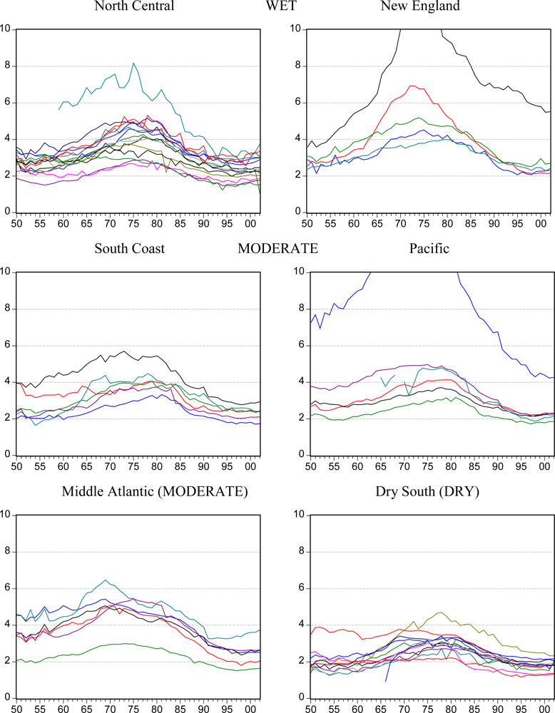
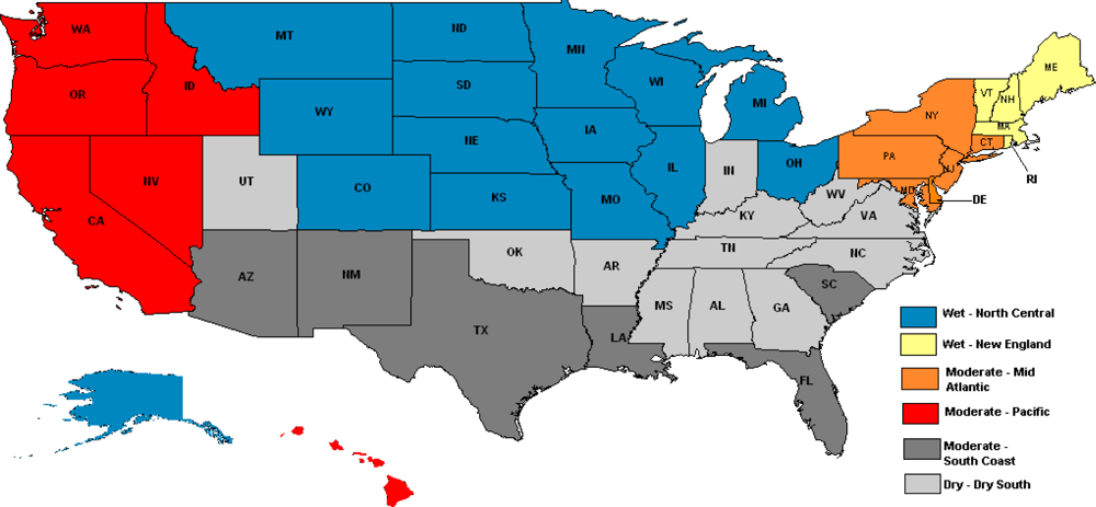
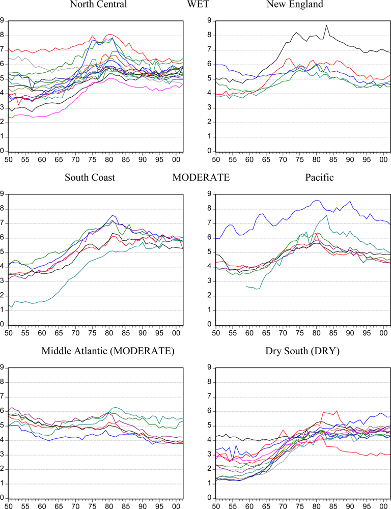
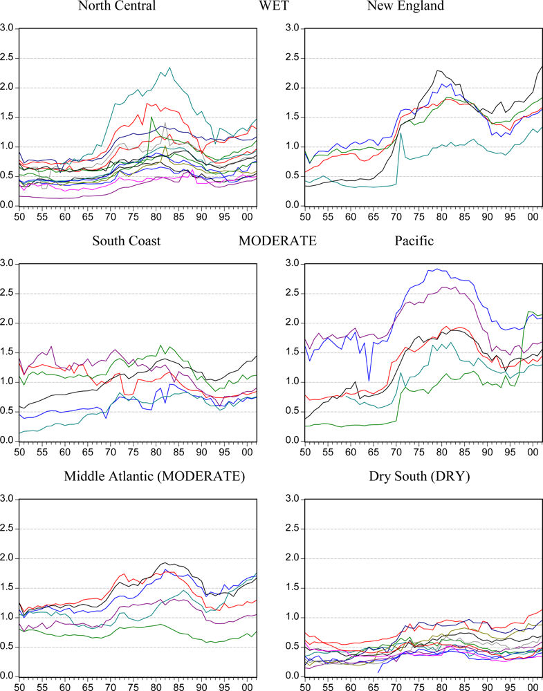
3. Results
- Wet
- North Central- Alaska, Colorado, Illinois, Iowa, Kansas, Michigan, Minnesota, Montana, Missouri, Ohio, Nebraska, North Dakota, South Dakota, Wisconsin, Wyoming
- New England- Maine, Massachusetts, New Hampshire, Rhode Island, Vermont
- Moderate
- Middle Atlantic- Connecticut, Delaware, Maryland, New Jersey, New York, Pennsylvania
- Pacific- California, Hawaii, Idaho, Nevada, Oregon, Washington
- South Coast- Arizona, Florida, Louisiana, New Mexico, South Carolina, Texas
- Dry
- Dry South- Alabama, Arkansas, Georgia, Indiana, Kentucky, Mississippi, North Carolina, Oklahoma, Tennessee, Utah, Virginia, West Virginia
4. Discussion
Acknowledgments
References
- Room, R. Region and urbanization as factors in drinking practices and problems. In The Pathogenesis of Alcoholism: Psychosocial Factors; Kissin, B, Begleiter, H, Eds.; Plenum Press: New York, NY, USA, 1983; Volume 6, pp. 555–604. [Google Scholar]
- Hilton, ME. Regional diversity in United States drinking practices. Br. J. Addict. 1988, 83, 519–532. [Google Scholar]
- Smith, PF; Remington, PL; Williamson, DF; Anda, RF. A comparison of alcohol sales data with survey data on self-reported alcohol use in 21 states. Am. J. Public Health 1990, 80, 309–312. [Google Scholar]
- Nelson, TF; Naimi, TS; Brewer, RD; Wechsler, H. The state sets the rate: the relationship among state-specific college binge drinking, state binge drinking rates, and selected state alcohol control policies. Am. J. Public Health 2005, 95, 441–446. [Google Scholar]
- Lindquist, C; Cockerham, WC; Hwang, S-S. Drinking patterns in the American Deep South. J. Stud. Alcohol 1999, 60, 663–666. [Google Scholar]
- Skog, O-J. The collectivity of drinking cultures: a theory of the distribution of alcohol consumption. Br. J. Addict. 1985, 80, 83–99. [Google Scholar]
- Holt, JB; Miller, JW; Naimi, TS; Sui, DZ. Religious affiliation and alcohol consumption in the United States. The Geographical Review 2006, 96, 523–542. [Google Scholar]
- Kerr, WC; Greenfield, TK; Bond, J; Ye, Y; Rehm, J. Age, period and cohort influences on beer, wine and spirits consumption trends in the US National Surveys. Addiction 2004, 99, 1111–1120. [Google Scholar]
- Hughes, A; Sathe, N; Spagnola, K. State Estimates of Substance Use from the 2005–2006 National Surveys on Drug Use and Health (DHHS Publication No SMA 08-4311, NSDUH Series H-33); Substance Abuse and Mental Health Services Administration, Office of Applied Studies: Rockville, MD, USA, 2008; p. 64. Available online: http://www.oas.samhsa.gov/2k6State/2k6state.pdf (accessed 13 July 2009). [Google Scholar]
- Centers for Disease Control and Prevention. Behavioral Risk Factor Surveillance System Survey Data; U.S. Department of Health and Human Services, Centers for Disease Control and Prevention: Atlanta, GA, USA, 2009. [Google Scholar]
- Kerr, WC; Brown, S; Greenfield, TK. National and state estimates of the mean ethanol content of beer sold in the U.S. and their impact on per capita consumption estimates: 1988 to 2001. Alcohol. Clin. Exp. Res. 2004, 28, 1524–1532. [Google Scholar]
- Kerr, WC; Greenfield, TK; Tujague, J; Brown, S. The alcohol content of wine consumed in the US and per capita consumption: new estimates reveal different trends. Alcohol. Clin. Exp. Res. 2006, 30, 516–522. [Google Scholar]
- Kerr, WC; Greenfield, TK; Tujague, J. Estimates of the mean alcohol concentration of the spirits, wine, and beer sold in the U.S. and per capita consumption: 1950–2002. Alcohol. Clin. Exp. Res. 2006, 30, 1583–1591. [Google Scholar]
- Kerr, WC; Greenfield, TK. Distribution of alcohol consumption and expenditures and the impact of improved measurement on coverage of alcohol sales in the 2000 National Alcohol Survey. Alcohol. Clin. Exp. Res. 2007, 31, 1714–1722. [Google Scholar]
- Granger, CWJ. Forecasting in Business and Economics; Academic Press: Boston, MA, USA, 1989. [Google Scholar]
- EViews. EViews 5 User's Guide; Quantitative Micro Software: Irvine, CA, USA, 2004. [Google Scholar]
- Miller, JW; Gfroerer, JC; Brewer, RD; Naimi, TS; Mokdad, A; Giles, WH. Prevalence of adult binge drinking: a comparison of two national drinking surveys. Am. J. Prev. Med. 2004, 27, 197–204. [Google Scholar]
- Kerr, WC; Greenfield, TK; Bond, J; Ye, Y; Rehm, J. Age-period-cohort modeling of alcohol volume and heavy drinking days in the US National Alcohol Surveys: divergence in younger and older adult trends. Addiction 2009, 104, 27–37. [Google Scholar]
- Wagenaar, AC; Toomey, TL. Effects of minimum drinking age laws: review and analyses of the literature from 1960 to 2000. J. Stud. Alcohol 2002, 14, 206–225. [Google Scholar]
- Wagenaar, AC; Maldonado-Molina, MM; Ma, L; Tobler, AL; Komro, KA. Effects of legal BAC limits on fatal crash involvement: analyses of 28 states from 1976 through 2002. J. Safety Res. 2007, 38, 493–499. [Google Scholar]
- Snortum, JR; Berger, DE. Drinking-driving compliance in the United States: percpetion and behavior in 1983 and 1986. J. Stud. Alcohol 1989, 50, 306–319. [Google Scholar]
- Michalak, L; Trocki, KF; Bond, J. Religion and alcohol in the U.S. National Alcohol Survey: how important is religion for abstention and drinking? Drug Alcohol Depend 2007, 87, 268–280. [Google Scholar]
- Caetano, R; Clark, CL; Tam, TW. Alcohol consumption among racial/ethnic minorities: theory and research. Alcohol Health Res. World 1998, 22, 233–241. [Google Scholar]
- Mulia, N; Ye, Y; Greenfield, TK; Zemore, SE. Disparities in alcohol-related problems among white, black, and Hispanic Americans. Alcohol. Clin. Exp. Res. 2009, 33, 654–662. [Google Scholar]
- Cremeens, JL; Nelson, D; Naimi, TS; Brewer, RD; Pearson, WS; Division of Adult and Community Health; National Center for Chronic Disease Prevention and Health Promotion; Chavez, PR; EIS Officer-CDC. Sociodemographic differences in binge drinking among adults—14 states, 2004. MMWR 2009, 58, 301–304. [Google Scholar]
- Dawson, DA. Beyond black, white and Hispanic: race, ethnic orgin and drinking patterns in the United States. J. Subst. Abuse 1998, 10, 321–339. [Google Scholar]
- Holder, HD. Community prevention of alcohol problems. Addict. Behav. 2000, 25, 843–859. [Google Scholar]
- Babor, TF; Caetano, R; Casswell, S; Edwards, G; Giesbrecht, NA; Graham, K; Grube, JW; Gruenewald, P; Hill, L; Holder, HD; Homel, R; Õsterberg, E; Rehm, J; Room, R; Rossow, I. Alcohol: No Ordinary Commodity: Research and Public Policy; Oxford University Press: New York, NY, USA, 2003. [Google Scholar]


| State | % | Ethanol Gallons per capita age 15+ 2005 | 2007 BRFSS 5+/4+ Monthly age 18+ % | Group Name | ||||
|---|---|---|---|---|---|---|---|---|
| 5+ Past Month age 12+ | 5+ Past Month ages 18–25 | 5+ Past Month age 26+ | Drinker Past Month age 12+ | Drinkers with 5+ in Past Month age 12+ | ||||
| North Dakota | 30.32 | 56.49 | 26.99 | 58.24 | 52.06 | 2.74 | 23.2 | NC |
| Wisconsin | 29.41 | 53.60 | 27.42 | 63.14 | 46.58 | 2.96 | 23.4 | NC |
| Montana | 28.57 | 54.85 | 25.60 | 56.71 | 50.38 | 2.74 | 17.1 | NC |
| Dist. of Columbia | 28.32 | 50.58 | 26.10 | 60.25 | 47.00 | 3.89 | 16.1 | none |
| South Dakota | 28.14 | 51.78 | 25.88 | 58.70 | 47.94 | 2.48 | 17.3 | NC |
| Minnesota | 27.86 | 50.35 | 25.80 | 61.74 | 45.12 | 2.40 | 14.3 | NC |
| Iowa | 27.14 | 50.85 | 24.83 | 53.09 | 51.12 | 2.19 | 19.9 | NC |
| Rhode Island | 27.12 | 51.19 | 24.75 | 61.23 | 44.29 | 2.52 | 18.6 | NE |
| Nebraska | 26.69 | 49.97 | 24.17 | 54.03 | 49.40 | 2.35 | 18.0 | NC |
| Vermont | 25.99 | 53.20 | 22.99 | 60.42 | 43.02 | 2.62 | 17.9 | NE |
| Illinois | 25.46 | 46.27 | 23.81 | 52.47 | 48.52 | 2.33 | 19.5 | NC |
| Kansas | 25.43 | 47.82 | 22.81 | 53.19 | 47.81 | 1.94 | 14.6 | NC |
| Michigan | 25.37 | 47.92 | 23.64 | 56.2 | 45.14 | 2.17 | 18.5 | NC |
| Wyoming | 25.21 | 49.58 | 22.23 | 56.36 | 44.73 | 2.74 | 16.8 | NC |
| Connecticut | 25.14 | 49.83 | 23.08 | 60.77 | 41.37 | 2.32 | 17.8 | MA |
| Massachusetts | 25.01 | 52.44 | 22.13 | 57.85 | 43.23 | 2.55 | 17.6 | NE |
| Colorado | 24.68 | 47.24 | 22.56 | 58.59 | 42.12 | 2.69 | 17.3 | NC |
| Ohio | 24.45 | 47.30 | 22.40 | 51.57 | 47.41 | 2.00 | 17.1 | NC |
| Texas | 24.06 | 40.99 | 22.90 | 49.49 | 48.62 | 2.24 | 15.3 | SC |
| Missouri | 23.86 | 46.90 | 21.55 | 49.91 | 47.81 | 2.38 | 16.2 | NC |
| New Hampshire | 23.83 | 50.98 | 21.20 | 60.79 | 39.20 | 4.21 | 15.5 | NE |
| Nevada | 23.75 | 42.40 | 22.59 | 52.00 | 45.67 | 3.70 | 16.9 | PA |
| Louisiana | 23.53 | 36.79 | 22.80 | 49.07 | 47.95 | 2.66 | 13.4 | SC |
| New York | 23.47 | 43.77 | 21.53 | 54.75 | 42.87 | 1.99 | 15.2 | MA |
| Pennsylvania | 23.09 | 45.09 | 21.14 | 52.30 | 44.15 | 2.12 | 16.2 | MA |
| Arizona | 22.87 | 40.85 | 21.38 | 54.37 | 42.06 | 2.47 | 15.0 | SC |
| Total U.S. | 22.82 | 42.02 | 21.20 | 51.37 | 44.42 | 2.27 | 15.8 | US |
| Washington | 22.80 | 41.24 | 21.23 | 54.45 | 41.87 | 2.24 | 15.8 | PA |
| Maine | 22.43 | 45.82 | 20.28 | 54.76 | 40.96 | 2.47 | 15.9 | NE |
| Florida | 22.34 | 38.13 | 21.52 | 53.43 | 41.81 | 2.72 | 14.2 | SC |
| New Jersey | 22.29 | 45.17 | 20.24 | 56.47 | 39.47 | 2.32 | 13.6 | MA |
| Idaho | 21.89 | 37.51 | 20.48 | 46.52 | 47.06 | 2.53 | 14.7 | PA |
| Kentucky | 21.79 | 38.77 | 20.48 | 42.47 | 51.31 | 1.83 | 8.2 | DS |
| Virginia | 21.79 | 41.07 | 20.29 | 51.86 | 42.02 | 2.10 | 15.9 | DS |
| Oregon | 21.61 | 39.52 | 19.92 | 54.67 | 39.53 | 2.53 | 15.6 | PA |
| Alaska | 21.58 | 35.89 | 20.84 | 52.74 | 40.92 | 2.73 | 19.2 | NC |
| Hawaii | 21.41 | 40.37 | 20.06 | 46.70 | 45.85 | 2.56 | 18.6 | PA |
| Delaware | 21.29 | 42.59 | 19.14 | 51.51 | 41.33 | 3.30 | 18.6 | MA |
| Oklahoma | 21.14 | 37.08 | 19.60 | 41.85 | 50.51 | 1.51 | 12.5 | DS |
| Indiana | 21.10 | 41.05 | 19.19 | 49.40 | 42.71 | 2.00 | 15.6 | DS |
| South Carolina | 20.88 | 36.71 | 19.88 | 45.26 | 46.13 | 2.46 | 13.9 | SC |
| California | 20.81 | 37.75 | 19.41 | 50.33 | 41.35 | 2.29 | 16.9 | PA |
| Arkansas | 20.71 | 38.19 | 18.84 | 42.61 | 48.60 | 1.82 | 10.4 | DS |
| Tennessee | 20.52 | 39.91 | 18.95 | 42.41 | 48.38 | 1.89 | 9.2 | DS |
| New Mexico | 20.30 | 37.43 | 18.54 | 45.83 | 44.29 | 2.39 | 12.3 | SC |
| Maryland | 20.20 | 37.50 | 18.91 | 53.14 | 38.01 | 2.19 | 12.6 | MA |
| Georgia | 19.65 | 35.21 | 18.51 | 44.85 | 43.81 | 2.06 | 12.6 | DS |
| North Carolina | 19.46 | 35.79 | 18.24 | 43.58 | 44.65 | 1.97 | 12.3 | DS |
| West Virginia | 18.90 | 40.93 | 16.53 | 36.40 | 51.92 | 1.74 | 9.8 | DS |
| Alabama | 18.74 | 33.77 | 17.42 | 42.45 | 44.15 | 1.97 | 11.0 | DS |
| Mississippi | 18.40 | 31.84 | 17.33 | 36.93 | 49.82 | 2.25 | 11.3 | DS |
| Utah | 17.38 | 28.31 | 16.04 | 32.40 | 53.64 | 1.30 | 9.8 | DS |
| Region | Number of states in group | Spirits within | Spirits outside | Beer within | Beer outside |
|---|---|---|---|---|---|
| Dry South Mid Atlantic North Central New England Pacific South Coast | 12 6 15 6 6 7 | 56.1% 66.7% 70.5% 60.0% 100.0% 80.0% | 73.1% 68.1% 70.2% 72.2% 74.4% 65.9% | 50.0% 20.0% 53.3% 80.0% 40.0% 33.3% | 44.0% 31.1% 44.8% 50.4% 47.8% 41.1% |
© 2010 by the authors; licensee Molecular Diversity Preservation International, Basel, Switzerland. This article is an open-access article distributed under the terms and conditions of the Creative Commons Attribution license (http://creativecommons.org/licenses/by/3.0/).
Share and Cite
Kerr, W.C. Categorizing US State Drinking Practices and Consumption Trends. Int. J. Environ. Res. Public Health 2010, 7, 269-283. https://doi.org/10.3390/ijerph7010269
Kerr WC. Categorizing US State Drinking Practices and Consumption Trends. International Journal of Environmental Research and Public Health. 2010; 7(1):269-283. https://doi.org/10.3390/ijerph7010269
Chicago/Turabian StyleKerr, William C. 2010. "Categorizing US State Drinking Practices and Consumption Trends" International Journal of Environmental Research and Public Health 7, no. 1: 269-283. https://doi.org/10.3390/ijerph7010269