Path Loss Determination Using Linear and Cubic Regression Inside a Classic Tomato Greenhouse

 ,
,  , ,
, ,
Abstract
:1. Introduction
Background
2. Materials and Methods
2.1. The Wireless Sensor Network
2.2. Received Signal Strength Indicator(RSSI)
2.3. Propagation with Line of Sight
- Loss in free space. When an electromagnetic wave (EM) propagates in free space, path loss can be calculated using the Friis equation, widely used by microwave link designers [42], which assumes the absence of obstacles in the vicinity [39,46]: , where Pr and Pt are the receiver and transmitter power respectively, f is the frequency of the radiation wave, c, the speed of light in the vacuum and d is the distance between the transmitter and the receiver [36,47]. The loss of the path in the free space means that the transceiver antennas, both transmitters and receivers, use communication with LOS, without obstructions or reflections of any kind. However, if the antennas are located close to the ground, the above equation is no longer valid, the reflection of the earth must be taken into account [18]. The power loss is usually expressed in terms of “path loss” (PL), defined as: PL = 10log10(Pt/Pr) [48] with Pt and Pr as power transmitted and received, respectively. Therefore, PL in free space can be expressed: PLFree-space(dB) = 20log(f) + 20log(d) − 147.56, the radiofrequency, f, is expressed in Hz and distance is expressed in meters [49,50].
- Two-ray propagation model. When the RF propagates near the ground with LOS, the flat ground wave (PE) propagation model can be used to define the path loss instead of the PLFree-space model. This model includes the effects of the reflection of the rays of the ground and the ray LOS, which is given by the equation: PLPE(dB) = 40log(d) − 20log(hT) − 20log(hR), where d is the distance between the transmitter and receiver antennas in meters, hT and hR are the elevations of the transceiver antennas in meters. The separation distance (d) in this model is much greater than hT and hR [45].
2.4. Total Loss
2.5. Link Budget
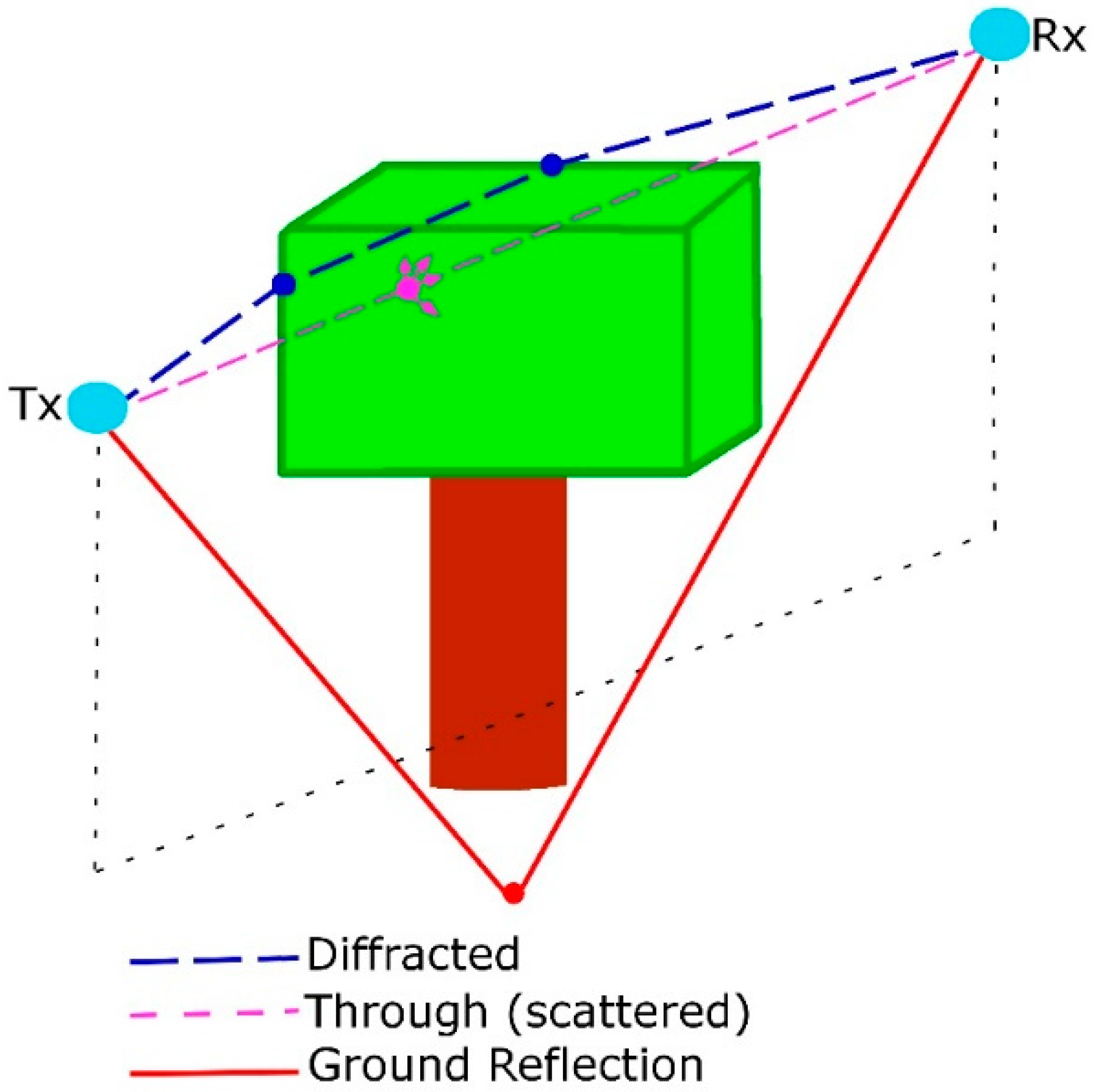
2.6. Propagation with Non Line of Sight (NLOS)
2.7. Propagation Model
2.8. Hardware
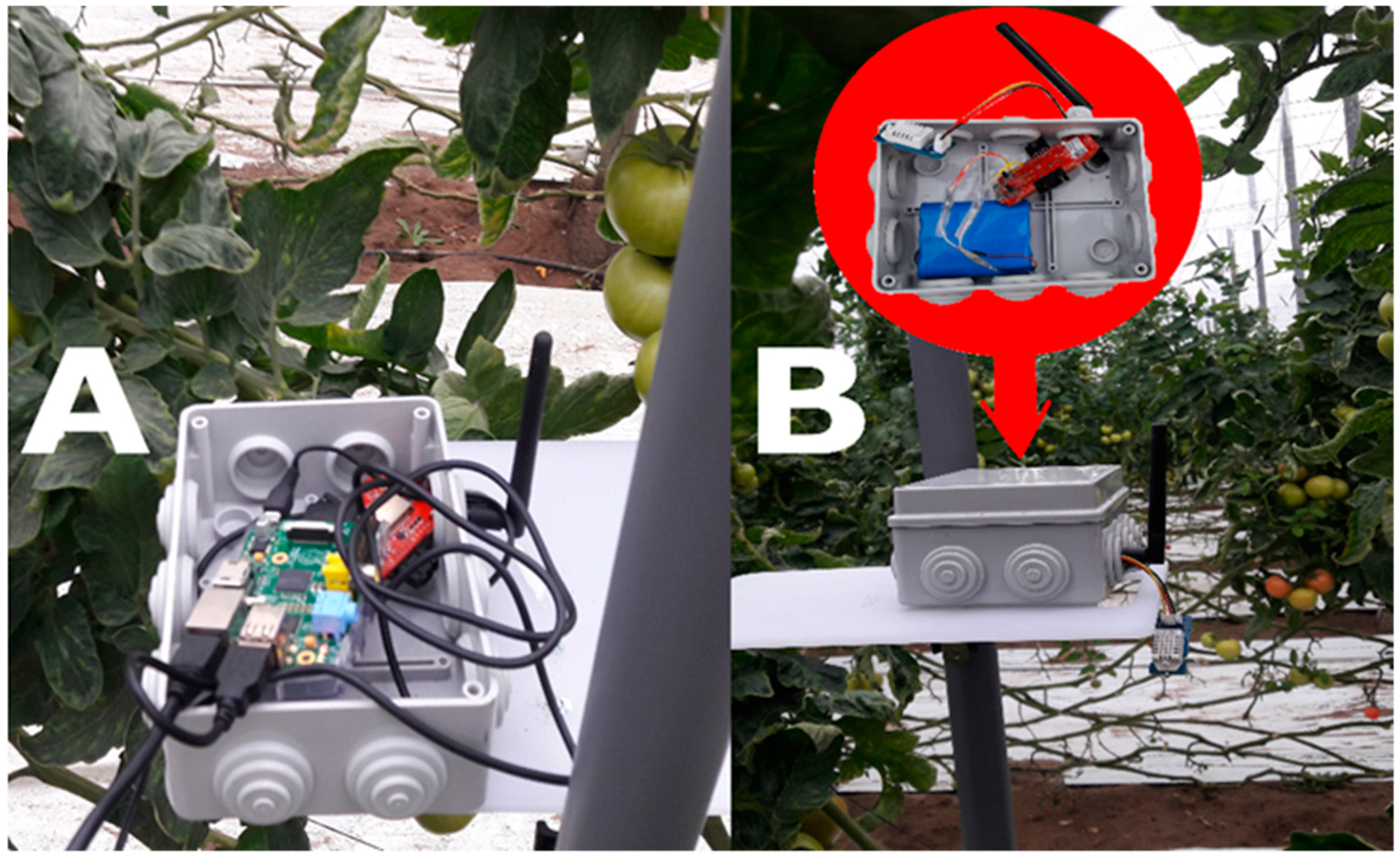
- Raspberry Pi. The Raspberry Pi 3 computer receives data from the sensor node through the sink node connected to its USB port. The electric energy, available inside the greenhouse, fed the Raspberry Pi uninterruptedly during the testing stage.
- Sensor and sink nodes. We used the Re-Mote nodes [74] that operate with the 2.4 GHz band (CC2538 System-on-Chip) for both the sensor node and the sink. The sink node is powered by the power provided by the USB cable connected to the Raspberry Pi computer (See Figure 2A), while the sensor node has a rechargeable Lithium-ion battery of 3.7 V and 6600 mAh (See Figure 2B).
2.9. Software
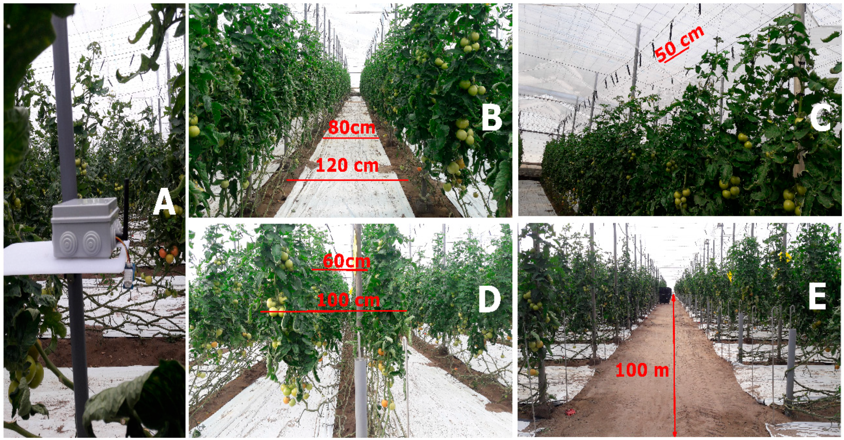
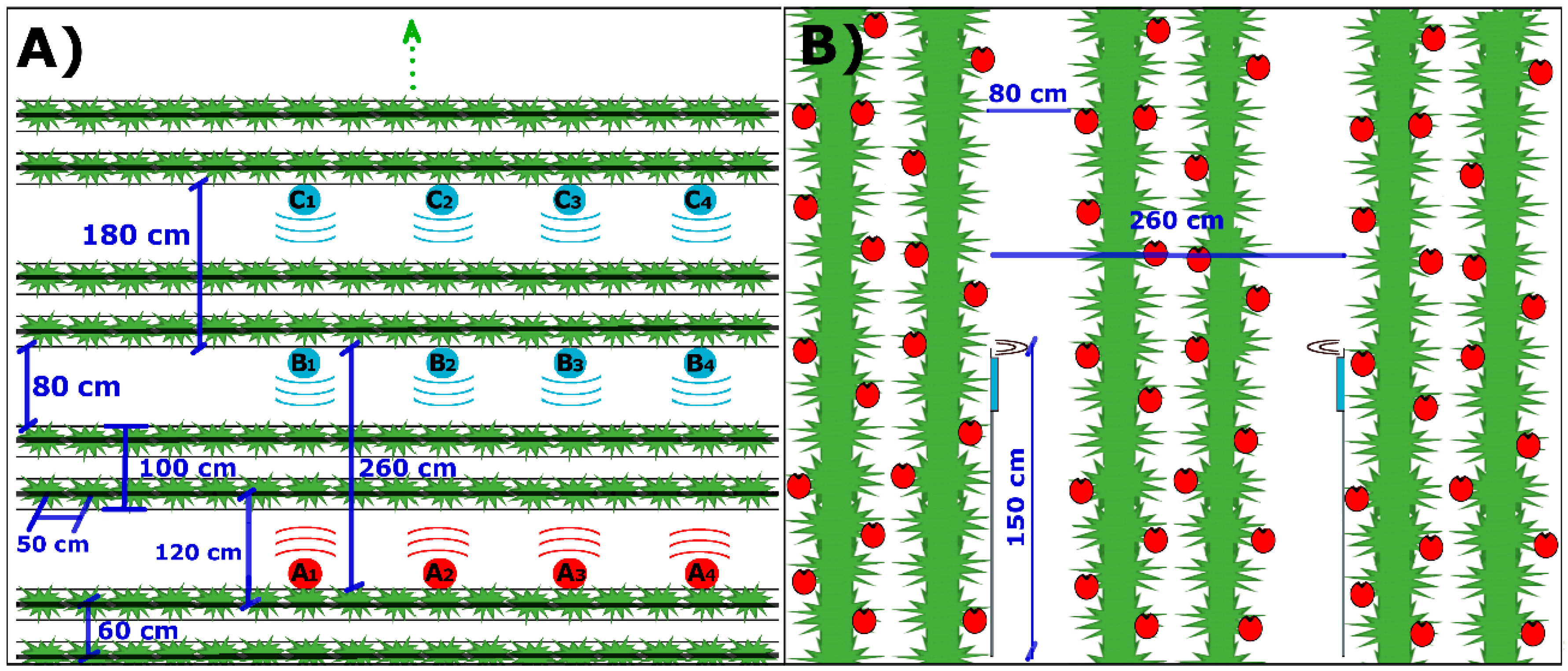
2.10. Test Environment
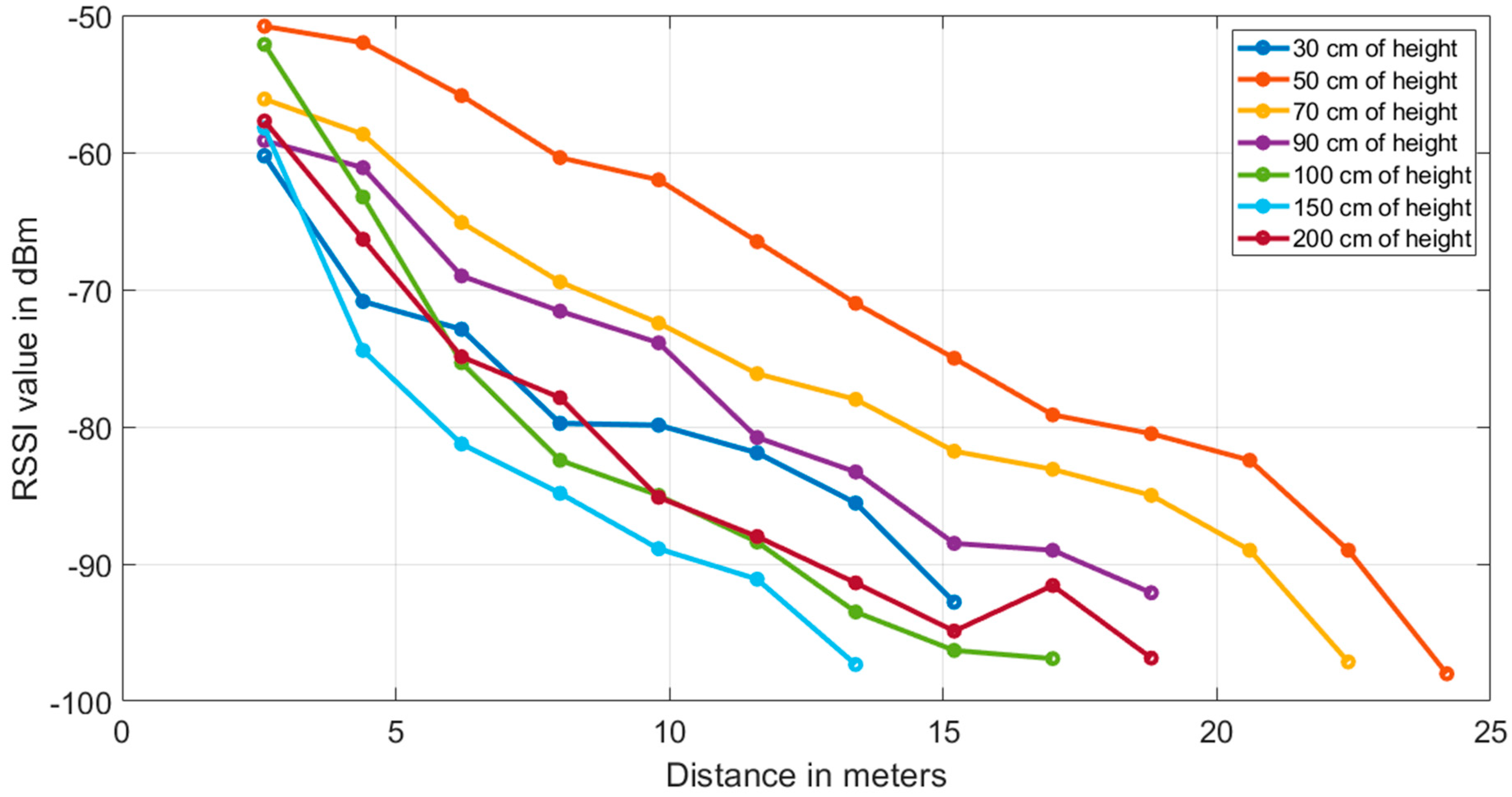
2.11. Field Tests
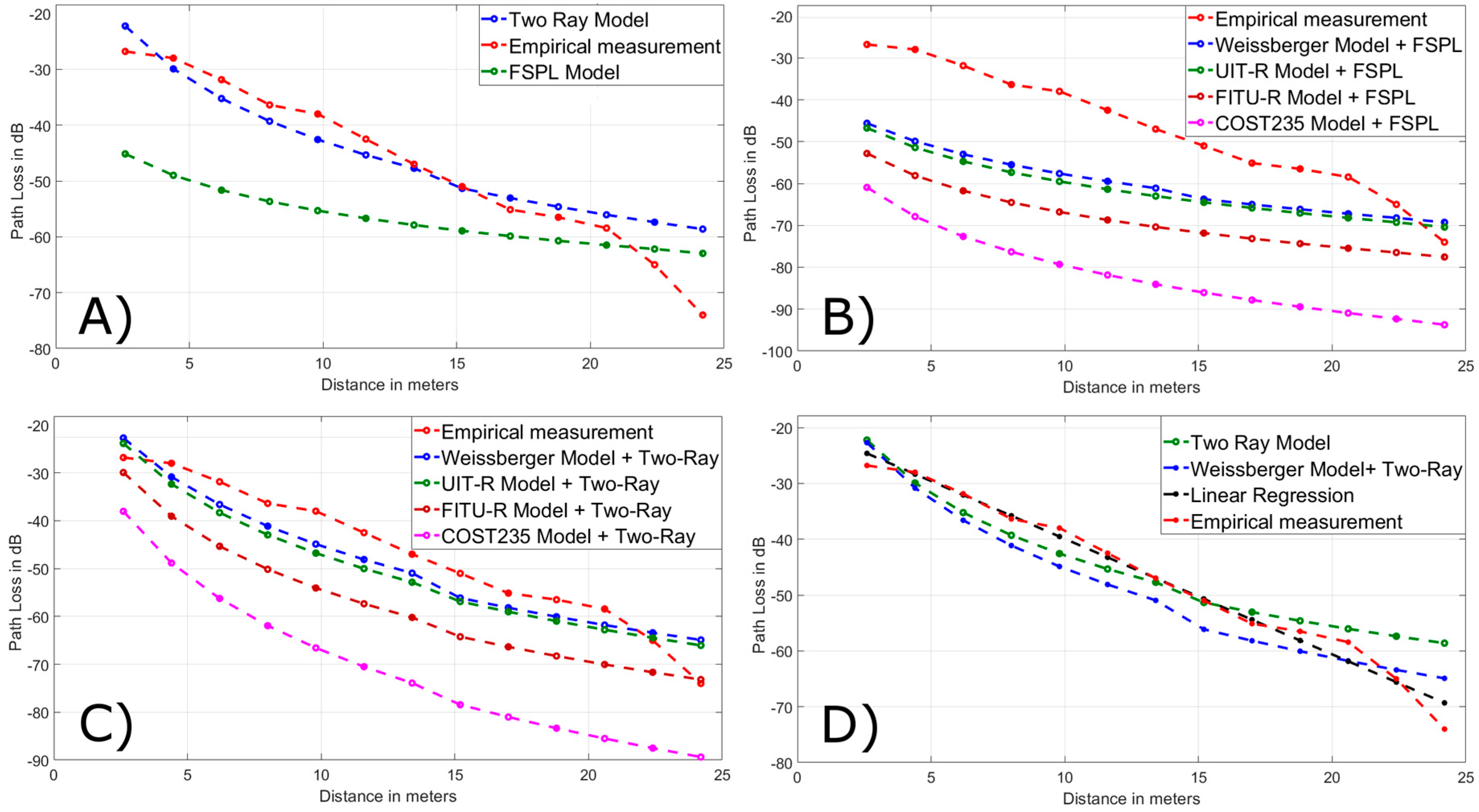
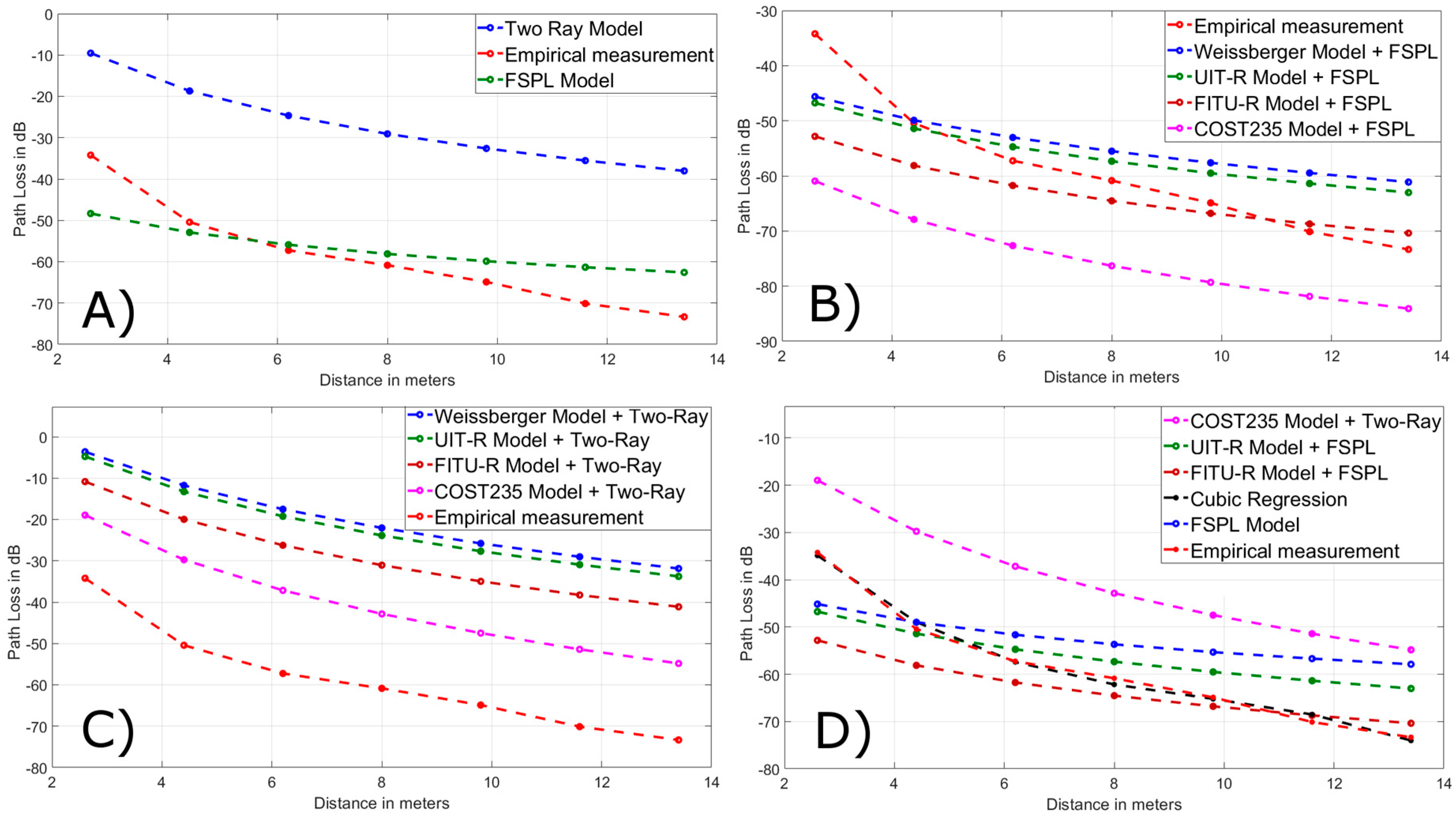
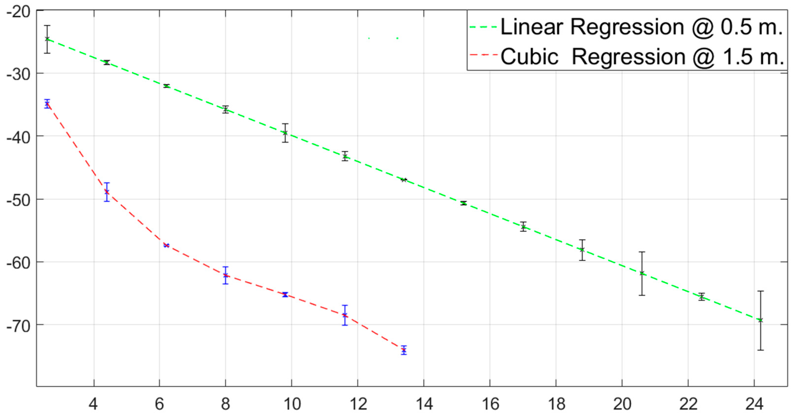
3. Results and Discussions
New Optimized Model with Verification of Values
4. Conclusions
Author Contributions
Funding
Conflicts of Interest
References
- Razafimandimby, C.; Loscrí, V.; Vegni, A.M.; Neri, A. Efficient Bayesian communication approach for smart agriculture applications. In Proceedings of the 2017 IEEE Vehicular Technology Conference, Toronto, ON, Canada, 24–27 September 2017; pp. 1–5. [Google Scholar] [CrossRef]
- Caicedo-Ortiz, J.G.; De-la-Hoz-Franco, E.; Morales Ortega, R.; Piñeres-Espitia, G.; Combita-Niño, H.; Estévez, F.; Cama-Pinto, A. Monitoring system for agronomic variables based in WSN technology on cassava crops. Comput. Electron. Agric. 2018, 145, 275–281. [Google Scholar] [CrossRef]
- Tzounis, A.; Katsoulas, N.; Bartzanas, T.; Kittas, C. Internet of Things in agriculture, recent advances and future challenges. Biosyst. Eng. 2017, 164, 31–48. [Google Scholar] [CrossRef]
- Sabri, N.; Mohammed, S.S.; Fouad, S.; Syed, A.A.; Al-Dhief, F.T.; Raheemah, A. Investigation of Empirical Wave Propagation Models in Precision Agriculture. MATEC Web Conf. 2018, 150, 06020. [Google Scholar] [CrossRef]
- Correia, F.P.; De Alencar, M.S.; Lopes, W.T.A.; De Assis, M.S.; Leal, B.G. Propagation analysis for wireless sensor networks applied to viticulture. Int. J. Antennas Propag. 2017, 2017, 7903839. [Google Scholar] [CrossRef]
- Yoshimura, R.; Hara, M.; Nishimura, T.; Yamada, C.; Shimasaki, H.; Kado, Y.; Ichida, M. Effect of vegetation on radio wave propagation in 920-MHz and 2.4-GHz bands. In Proceedings of the Asia-Pacific Microwave Conference (APMC), New Delhi, India, 5–9 December 2016. [Google Scholar] [CrossRef]
- Correia, F.P.; Alencar, M.S.; Carvalho, F.B.S.; Lopes, W.T.A.; Leal, B.G. Propagation analysis in precision agriculture environment using XBee devices. In Proceedings of the SBMO/IEEE MTT-S International Microwave and Optoelectronics Conference, Rio de Janeiro, Brazil, 4–7 August 2013. [Google Scholar] [CrossRef]
- Li, J.; Shen, C. Energy conservative Wireless Sensor Networks for black pepper monitoring in tropical area. In Proceedings of the IEEE Global High Tech Congress on Electronics (GHTCE), Shenzhen, China, 17–19 November 2013; pp. 159–164. [Google Scholar] [CrossRef]
- Montoya, F.G.; Gomez, J.; Manzano-Agugliaro, F.; Cama, A.; García-Cruz, A.; De La Cruz, J.L. 6LoWSoft: A software suite for the design of outdoor environmental measurements. J. Food Agric. Environ. 2013, 11, 2584–2586. [Google Scholar]
- Holvoet, K.; Sampers, I.; Seynnaeve, M.; Jacxsens, L.; Uyttendaele, M. Agricultural and management practices and bacterial contamination in greenhouse versus open field lettuce production. Int. J. Environ. Res. Public Health 2015, 12, 32–63. [Google Scholar] [CrossRef] [PubMed]
- Sabri, N.; Aljunid, S.A.; Salim, M.S.; Kamaruddin, R.; Ahmad, R.B.; Malek, M.F. Path loss analysis of WSN wave propagation in vegetation. J. Phys. Conf. Ser. 2013, 423, 012063. [Google Scholar] [CrossRef]
- Paul, B.S.; Rimer, S. A foliage scatter model to determine topology of wireless sensor network. In Proceedings of the International Conference on Radar, Communication and Computing (ICRCC), Tiruvannamalai, India, 21–22 December 2012; pp. 324–328. [Google Scholar] [CrossRef]
- Liu, H.; Meng, Z.; Wang, M. A wireless sensor network for cropland environmental monitoring. In Proceedings of the International Conference on Networks Security, Wireless Communications and Trusted Computing (NSWCTC), Wuhan, China, 25–26 April 2009; Volume 1, pp. 65–68. [Google Scholar] [CrossRef]
- Piñeres-Espitia, G.; Cama-Pinto, A.; De La Rosa Morrón, D.; Estevez, F.; Cama-Pinto, D. Design of a low cost weather station for detecting environmental changes. Espacios 2017, 38, 13. [Google Scholar]
- Sánchez, J.A.; Reca, J.; Martínez, J. Water productivity in a mediterranean semi-arid greenhouse district. Water Resour. Manag. 2015, 29, 5395–5411. [Google Scholar] [CrossRef]
- De Pablo-Valenciano, J.; Giacinti-Battistuzzi, M.A.; Tassile, V.; García-Azcárate, T. Changes in the business model for Spanish fresh tomato trade. Span. J. Agric. Res. 2017, 15, e0101. [Google Scholar] [CrossRef] [Green Version]
- Marín, P.; Valera, D.L.; Molina-Aiz, F.D.; López, A.; Belmonte, L.J.; Moreno, M.A. Influence of different heating systems on the development, production and quality of a tomato crop. ITEA Inf. Tec. Econ. Agrar. 2016, 112, 375–391. [Google Scholar] [CrossRef]
- Vougioukas, S.; Anastassiu, H.T.; Regen, C.; Zude, M. Influence of foliage on radio path losses (PLs) for Wireless Sensor Network (WSN) planning in orchards. Biosyst. Eng. 2013, 114, 454–465. [Google Scholar] [CrossRef]
- Raheemah, A.; Sabri, N.; Salim, M.S.; Ehkan, P.; Ahmad, R.B. New empirical path loss model for wireless sensor networks in mango greenhouses. Comput. Electron. Agric. 2016, 127, 553–560. [Google Scholar] [CrossRef]
- Mancuso, M.; Bustaffa, F. A Wireless Sensors Network for monitoring environmental variables in a tomato greenhouse. In Proceedings of the IEEE International Workshop on Factory Communication Systems (WFCS), Torino, Italy, 28–30 June 2006; pp. 107–110. [Google Scholar]
- Erazo-Rodas, M.; Sandoval-Moreno, M.; Muñoz-Romero, S.; Huerta, M.; Rivas-Lalaleo, D.; Naranjo, C.; Rojo-álvarez, J.L. Multiparametric monitoring in equatorian tomato greenhouses (I): Wireless sensor network benchmarking. Sensors 2018, 18, 2555. [Google Scholar] [CrossRef] [PubMed]
- Zhou, H.; Qi, H.; Banhazi, T.M.; Low, T. An integrated WSN and mobile robot system for agriculture and environment applications. In Lecture Notes of the Institute for Computer Sciences, Social-Informatics and Telecommunications Engineering, LNICST; Springer: Cham, Switzerland, 2014; Volume 131, pp. 30–36. [Google Scholar] [CrossRef]
- Foerster, A.; Udugama, A.; Görg, C.; Kuladinithi, K.; Timm-Giel, A.; Cama-Pinto, A. A novel data dissemination model for organic data flows. In Lecture Notes of the Institute for Computer Sciences, Social-Informatics and Telecommunications Engineering, LNICST; Springer: Cham, Switzerland, 2015; Volume 158, pp. 239–252. [Google Scholar] [CrossRef]
- Chaiwatpongsakorn, C.; Lu, M.; Keener, T.C.; Khang, S.-J. The deployment of carbon monoxide wireless sensor network (CO-WSN) for ambient air monitoring. Int. J. Environ. Res. Public Health 2014, 11, 6246–6264. [Google Scholar] [CrossRef]
- Queiroz, D.V.; Alencar, M.S.; Gomes, R.D.; Fonseca, I.E.; Benavente-Peces, C. Survey and systematic mapping of industrial Wireless Sensor Networks. J. Netw. Comput. Appl. 2017, 97, 96–125. [Google Scholar] [CrossRef]
- Stewart, J.; Stewart, R.; Kennedy, S. Internet of Things—Propagation modelling for precision agriculture applications. In Proceedings of the Wireless Telecommunications Symposium, Chicago, IL, USA, 26–28 April 2017. [Google Scholar] [CrossRef]
- Zhang, H.; Li, H. Node localization technology of wireless sensor network based on RSSI algorithm. Int. J. Online Eng. 2016, 12, 51–57. [Google Scholar] [CrossRef]
- Guo, X.-M.; Yang, X.-T.; Chen, M.-X.; Li, M.; Wang, Y.-A. A model with leaf area index and apple size parameters for 2.4 GHz radio propagation in apple orchards. Precis. Agric. 2015, 16, 180–200. [Google Scholar] [CrossRef]
- Galvan-Tejada, G.M.; Duarte-Reynoso, E.Q.; Flores-Leal, R. Standard conditions of propagation for wireless sensor networks in an inhomogeneous vegetation environment. In Proceedings of the IEEE Antennas and Propagation Society, AP-S International Symposium (Digest), Orlando, FL, USA, 7–13 July 2013; pp. 2014–2015. [Google Scholar] [CrossRef]
- Galvan-Tejada, G.M.; Duarte-Reynoso, E.Q. A study based on the Lee propagation model for a wireless sensor network on a non-uniform vegetation environment. In Proceedings of the IEEE Latin-America Conference on Communications (LATINCOM), Cuenca, Ecuador, 7–9 November 2012. [Google Scholar] [CrossRef]
- Li, T.; Zhang, M.; Ji, Y.H.; Sha, S.; Jiang, Y.Q.; Li, M.Z. Management of CO2 in a tomato greenhouse using WSN and BPNN techniques. Int. J. Agric. Boil. Eng. 2015, 8, 43–51. [Google Scholar] [CrossRef]
- Liu, H.; Meng, Z.; Shang, Y. Sensor nodes placement for farmland environmental monitoring applications. In Proceedings of the 5th International Conference on Wireless Communications, Networking and Mobile Computing WiCOM, Beijing, China, 24–26 September 2009. [Google Scholar] [CrossRef]
- Gay-Fernandez, J.A.; Cuinas, I. Short-term modeling in vegetation media at wireless network frequency bands. IEEE Trans. Antennas Propag. 2014, 62, 3330–3337. [Google Scholar] [CrossRef]
- Li, Z.; Wang, N.; Hong, T. RF propagation patterns at 915 MHZ and 2.4 GHZ bands for in-field wireless sensor networks. Trans. ASABE 2013, 56, 787–796. [Google Scholar]
- Haber, R.; Peter, A.; Otero, C.E.; Kostanic, I.; Ejnioui, A. A support vector machine for terrain classification in on-demand deployments of wireless sensor networks. In Proceedings of the 7th Annual IEEE International Systems Conference (SysCon), Orlando, FL, USA, 15–18 April 2013; pp. 841–846. [Google Scholar] [CrossRef]
- De Sales Bezerra, T.; De Sousa, J.A.R.; Da Silva Eleuterio, S.A.; Rocha, J.S. Accuracy of propagation models to power prediction in WSN ZigBee applied in outdoor environment. In Proceedings of the 6th Argentine Conference on Embedded Systems (CASE), Buenos Aires, Argentina, 12–14 August 2015; pp. 19–24. [Google Scholar] [CrossRef]
- Rao, Y.; Jiang, Z.-H.; Lazarovitch, N. Investigating signal propagation and strength distribution characteristics of wireless sensor networks in date palm orchards. Comput. Electron. Agric. 2016, 124, 107–120. [Google Scholar] [CrossRef]
- Zhang, X.; Wu, Y.; Wei, X. Localization algorithms in wireless sensor networks using nonmetric multidimensional scaling with RSSI for precision agriculture. In Proceedings of the 2nd International Conference on Computer and Automation Engineering (ICCAE), Singapore, 26–28 February 2010; Volume 5, pp. 556–559. [Google Scholar] [CrossRef]
- Anastassiu, H.T.; Vougioukas, S.; Fronimos, T.; Regen, C.; Petrou, L.; Zude, M.; Käthner, J. A computational model for path loss in wireless sensor networks in orchard environments. Sensors 2014, 14, 5118–5135. [Google Scholar] [CrossRef]
- Zuniga, M.; Krishnamachari, B. Analyzing the transitional region in low power wireless links. In Proceedings of the First Annual IEEE Communications Society Conference on Sensor and Ad Hoc Communications and Networks, IEEE SECON, Santa Clara, CA, USA, 4–7 October 2004; pp. 517–526. [Google Scholar]
- Ngandu, G.; Nomatungulula, C.; Rimer, S.; Paul, B.S.; Ouahada, K.; Twala, B. Evaluating effect of foliage on link reliability of wireless signal. In Proceedings of the IEEE International Conference on Industrial Technology, Cape Town, South Africa, 25–28 February 2013; pp. 1528–1533. [Google Scholar] [CrossRef]
- Cama-Pinto, A.; Piñeres-Espitia, G.; Caicedo-Ortiz, J.; Ramírez-Cerpa, E.; Betancur-Agudelo, L.; Gómez-Mula, F. Received strength signal intensity performance analysis in wireless sensor network using Arduino platform and XBee wireless modules. Int. J. Distrib. Sens. Netw. 2017, 13. [Google Scholar] [CrossRef] [Green Version]
- Wang, J.; Peng, Y.; Li, P. Propagation characteristics of radio wave in plastic greenhouse. In IFIP Advances in Information and Communication Technology; Springer: Cham, Switzerland, 2016; Volume 478, pp. 208–215. [Google Scholar] [CrossRef]
- Huang, C.-N.; Chan, C.-T. A ZigBee-based location-aware fall detection system for improving elderly telecare. Int. J. Environ. Res. Public Health 2014, 11, 4233–4248. [Google Scholar] [CrossRef] [PubMed]
- Rogers, N.C.; Seville, A.; Richter, J.; Ndzi, D.; Savage, N.; Caldeirinha, R.F.S.; Shukla, A.K.; Al-Nuaimi, M.O.; Craig, K.; Vilar, E.; et al. A Generic Model of 1–60 GHz Radio Propagation through Vegetation—Final Report; UK Radiocommunications Agency: Worcestershire, UK, 2002; p. 134. [Google Scholar]
- Friis, H.T. A Note on a Simple Transmission Formula. Proc. IRE 1946, 34, 254–256. [Google Scholar] [CrossRef]
- Afsharinejad, A.; Davy, A.; Jennings, B.; Rasmann, S.; Brennan, C. A path-loss model incorporating shadowing for THz band propagation in vegetation. In Proceedings of the IEEE Global Communications Conference (GLOBECOM), San Diego, CA, USA, 6–10 December 2015. [Google Scholar] [CrossRef]
- Zhang, W.; He, Y.; Liu, F.; Miao, C.; Sun, S.; Liu, C.; Jin, J. Research on WSN channel fading model and experimental analysis in orchard environment. In IFIP Advances in Information and Communication Technology; 369 AICT (PART 2); Springer: Berlin/Heidelberg, Germany, 2012; pp. 326–333. [Google Scholar] [CrossRef]
- Mahesh, G.; Balachander, D.; Rao, T.R. RF propagation measurements in agricultural fields for Wireless Sensor Communications. In Proceedings of the IEEE International Conference on Circuit, Power and Computing Technologies (ICCPCT), Nagercoil, India, 20–21 March 2013; pp. 808–812. [Google Scholar] [CrossRef]
- Rama Rao, T.; Balachander, D.; Tiwari, N. UHF short-range pathloss measurements in forest & plantation environments for wireless sensor networks. In Proceedings of the IEEE International Conference on Communication Systems (ICCS), Singapore, 21–23 November 2012; pp. 194–198. [Google Scholar] [CrossRef]
- Agrawal, S.K.; Garg, P. Calculation of channel capacity and rician factor in the presence of vegetation in higher altitude platforms communication systems. In Proceedings of the 15th International Conference on Advanced Computing and Communications (ADCOM), Guwahati, India, 18–21 December 2007; pp. 243–248. [Google Scholar]
- Galvan-Tejada, G.M.; Duarte-Reynoso, E.Q. Some guidelines to simulate wireless sensor networks in a propagation environment with non-uniform vegetation. Int. J. Sens. Netw. 2015, 17, 40–51. [Google Scholar] [CrossRef]
- Wong, T.W. Electrical, magnetic, photomechanical and cavitational waves to overcome skin barrier for transdermal drug delivery. J. Control. Release 2014, 193, 257–269. [Google Scholar] [CrossRef]
- Gay-Fernandez, J.A.; Cuinas, I. Peer to peer propagation in vegetation media for wireless sensor networks. In Proceedings of the IEEE Antennas and Propagation Society, AP-S International Symposium (Digest), Chicago, IL, USA, 8–14 July 2012. [Google Scholar] [CrossRef]
- Tewari, R.K.; Swarup, S.; Roy, M.N. Radio Wave Propagation Through Rain Forests of India. IEEE Trans. Antennas Propag. 1990, 38, 433–449. [Google Scholar] [CrossRef]
- Savage, N.; Ndzi, D.; Seville, A.; Vilar, E.; Austin, J. Radio wave propagation through vegetation: Factors influencing signal attenuation. Radio Sci. 2003, 38. [Google Scholar] [CrossRef] [Green Version]
- Mestre, P.; Ribeiro, J.; Serodio, C.; Monteiro, J. Propagation of IEEE802.15.4 in vegetation. In Proceedings of the World Congress on Engineering (WCE), London, UK, 6–8 July 2011; Volume 2, pp. 1786–1791. [Google Scholar]
- Anderson, C.R.; Volos, H.I.; Buehrer, R.M. Characterization of low-antenna ultrawideband propagation in a forest environment. IEEE Trans. Veh. Technol. 2013, 62, 2878–2895. [Google Scholar] [CrossRef]
- Shaik, M.; Kabanni, A.; Nazeema, N. Millimeter wave propagation measurments in forest for 5G Wireless sensor communications. In Proceedings of theMediterranean Microwave Symposium, Abu Dhabi, UAE, 14–16 November 2017. [Google Scholar] [CrossRef]
- Ndzi, D.L.; Harun, A.; Ramli, F.M.; Kamarudin, M.L.; Zakaria, A.; Shakaff, A.Y.M.; Jaafar, M.N.; Zhou, S.; Farook, R.S. Wireless sensor network coverage measurement and planning in mixed crop farming. Comput. Electron. Agric. 2014, 105, 83–94. [Google Scholar] [CrossRef] [Green Version]
- Khairunnniza-Bejo, S.; Ramli, N.; Muharam, F.M. Wireless sensor network (WSN) applications in plantation canopy areas: A review. Asian J. Sci. Res. 2018, 11, 151–161. [Google Scholar] [CrossRef]
- Zakaria, Y.; Ivanek, L. Propagation measurements and estimation of channel propagation models in urban environment. KSII Trans. Internet Inf. Syst. 2017, 11, 2453–2467. [Google Scholar] [CrossRef]
- Oroza, C.A.; Zhang, Z.; Watteyne, T.; Glaser, S.D. A machine-learning-based connectivity model for complex terrain large-scale low-power wireless deployments. IEEE Trans. Cogn. Commun. Netw. 2017, 3, 576–584. [Google Scholar] [CrossRef]
- Rahim, H.M.; Leow, C.Y.; Rahman, T.A. Millimeter wave propagation through foliage: Comparison of models. In Proceedings of the IEEE 12th Malaysia International Conference on Communications (MICC), Kuching, Malaysia, 23–25 November 2015; pp. 236–240. [Google Scholar] [CrossRef]
- Cuiñas, I.; Gay-Fernández, J.A. A proposal on spatial diversity in emergency communications within forest environments. In Proceedings of the 8th European Conference on Antennas and Propagation (EuCAP), The Hague, The Netherlands, 6–11 April 2014; pp. 1295–1298. [Google Scholar] [CrossRef]
- Balachander, D.; Rao, T.R.; Mahesh, G. RF propagation investigations in agricultural fields and gardens for wireless sensor communications. In Proceedings of the IEEE Conference on Information and Communication Technologies (ICT), Thuckalay, India, 11–12 April 2013; pp. 755–759. [Google Scholar] [CrossRef]
- Rahman, N.Z.A.; Tan, K.G.; Omer, A.; Rahman, T.A.; Reza, A.W. Radio propagation studies at 5.8 GHZ for point-to-multipoint applications incorporating vegetation effect. Wirel. Pers. Commun. 2013, 72, 709–728. [Google Scholar] [CrossRef]
- Mani, F.; Oestges, C. A ray based method to evaluate scattering by vegetation elements. IEEE Trans. Antennas Propag. 2012, 60, 4006–4009. [Google Scholar] [CrossRef]
- Chee, K.L.; Torrico, S.A.; Kurner, T. Foliage attenuation over mixed terrains in rural areas for broadband wireless access at 3.5 GHz. IEEE Trans. Antennas Propag. 2011, 59, 2698–2706. [Google Scholar] [CrossRef]
- Meng, Y.S.; Lee, Y.H. Investigations of foliage effect on modern wireless communication systems: A review. Prog. Electromagn. Res. 2010, 105, 313–332. [Google Scholar] [CrossRef]
- Mestre, P.; Serôdio, C.; Morais, R.; Azevedo, J.; Melo-Pinto, P. Vegetation growth detection using wireless sensor networks. In Proceedings of the WCE 2010—World Congress on Engineering, London, UK, 30 June–2 July 2010; Volume 1, pp. 802–807. [Google Scholar]
- Sabri, N.; Aljunid, S.A.; Ahmad, R.B.; Malek, M.F.A.; Kamaruddin, R.; Salim, M.S. Wireless sensor network wave propagation in vegetation: Review and simulation. In Proceedings of the LAPC—Loughborough Antennas and Propagation Conference, Loughborough, UK, 12–13 November 2012. [Google Scholar] [CrossRef]
- Rahman, N.Z.A.; Tan, K.G.; Rahman, T.A.; Idris, I.F.M.; Hamzah, N.A.A. Modeling of Dynamic Effect of Vegetation for Fixed Wireless Access System. Wirel. Pers. Commun. 2017, 96, 1329–1354. [Google Scholar] [CrossRef]
- Zolertia. Z1 Datasheet. 2017. Available online: http://github.com/Zolertia/Resources/wiki/RE-Mote (accessed on 21 March 2019).
- Cama-Pinto, A.; Piñeres-Espitia, G.; Comas-González, Z.; Vélez-Zapata, J.; Gómez-Mula, F. Design of a monitoring network of meteorological variables related to tornadoes in Barranquilla-Colombia and its metropolitan area. Ingeniare 2017, 25, 585–598. [Google Scholar]
- Cama-Pinto, A.; Piñeres-Espitia, G.; Zamora-Musa, R.; Acosta-Coll, M.; Caicedo-Ortiz, J.; Sepúlveda-Ojeda, J. Design of a wireless sensor network for monitoring of flash floods in the city of Barranquilla Colombia. Ingeniare 2016, 24, 581–599. [Google Scholar]
- Zennaro, M.; Bagula, A.; Gascon, D.; Noveleta, A.B. Long distance wireless sensor networks: Simulation vs. reality. In Proceedings of the 4th ACM Workshop on Networked Systems for Developing Regions, NSDR ’10, San Francisco, CA, USA, 15 June 2010. [Google Scholar] [CrossRef]
- Montoya, F.G.; Gómez, J.; Cama, A.; Zapata-Sierra, A.; Martínez, F.; De La Cruz, J.L.; Manzano-Agugliaro, F.A. Monitoring system for intensive agriculture based on mesh networks and the android system. Comput. Electron. Agric. 2013, 99, 14–20. [Google Scholar] [CrossRef]
- Cama-Pinto, A.; Gil-Montoya, F.; Gómez-López, J.; García-Cruz, A.; Manzano-Agugliaro, F. Wireless surveillance sytem for greenhouse crops. DYNA 2014, 81, 164–170. [Google Scholar] [CrossRef]


| Model | Equation |
|---|---|
| The modified exponential decay model of Weissberger | LWeiss = 0.45f0.284d, 0 m < d < 14 m LWeiss = 1.33f0.284d0.558, 14 m < d < 400 m The frequency f in GHz and the depth of the trees, d, in meters. Applicable at frequencies of 0.23–95 GHz. |
| Loss factor of the ITU-R model | LITU-R = 0.2f0.3 d0.6, d < 400 m. The frequency f in MHz and the depth of the trees, d, in meters. Applicable to the frequency of 0.2–95 GHz. |
| Loss factor of the COST235 model | LCOST235 = 26.6f−0.2d0.5out-of-leaf LCOST235 = 15.6f−0.009d0.26in-leaf f is the transmission frequency (MHz), d is the depth of the trees in meters. Applicable to the frequency of 0.2–95 GHz |
| FITU-R | LFITU-R = 0.37f−018d0.59out-of-leaf LFITU-R = 0.39f−0.39d0.25in-leaf f is the frequency in MHz and d is the tree depth in meter, based on millimeter VHF wave measurement data on a short foliage depth (maximum of 400 m) |
| Model | Distance (m) | ||||||||||||
|---|---|---|---|---|---|---|---|---|---|---|---|---|---|
| 2.6 | 4.4 | 6.2 | 8 | 9.8 | 11.6 | 13.4 | 15.2 | 17.0 | 18.8 | 20.6 | 22.4 | 24.2 | |
| Empirical PL (dB) at 0.5 m | 26.8 | 28 | 31.86 | 36.38 | 38 | 42.5 | 47 | 51 | 55.13 | 56.5 | 58.44 | 65 | 74 |
| Empirical PL (dB) at 1.5 m | 34.22 | 50.43 | 57.25 | 60.85 | 64.89 | 70.11 | 73.33 | - | - | - | - | - | - |
| % Error | Distance (m) | ||||||||||||
|---|---|---|---|---|---|---|---|---|---|---|---|---|---|
| 2.6 | 4.4 | 6.2 | 8 | 9.8 | 11.6 | 13.4 | 15.2 | 17.0 | 18.8 | 20.6 | 22.4 | 24.2 | |
| FSPL | 40.64 | 42.84 | 38.30 | 32.21 | 31.30 | 25.04 | 18.81 | 13.46 | 7.92 | 6.94 | 4.95 | 4.52 | 17.52 |
| Two-Ray | 20.44 | 6.44 | 9.57 | 7.41 | 10.75 | 6.27 | 1.52 | 0.65 | 3.91 | 3.44 | 4.25 | 13.27 | 26.25 |
| Weissberger + Two Ray | 17.99 | 9.24 | 12.99 | 11.56 | 15.34 | 11.66 | 7.76 | 9.15 | 5.25 | 5.93 | 5.43 | 2.51 | 13.99 |
| Linear Regression | 8.81 | 1.25 | 0.68 | 1.62 | 3.85 | 1.73 | 0.06 | 0.61 | 1.31 | 2.82 | 5.53 | 0.89 | 6.77 |
| % Error | Distance (m) | ||||||
|---|---|---|---|---|---|---|---|
| 2.6 | 4.4 | 6.2 | 8 | 9.8 | 11.6 | 13.4 | |
| FSPL | 29.22 | 4.69 | 2.43 | 4.72 | 8.39 | 14.31 | 17.17 |
| Two-Ray | 258.13 | 169.76 | 132.23 | 109.25 | 99.02 | 97.30 | 92.77 |
| COST235 + 2-Ray | 80.52 | 69.52 | 54.08 | 42.02 | 36.65 | 36.36 | 33.75 |
| UIT-R + FSPL | 26.79 | 1.9 | 4.62 | 6.13 | 9.05 | 14.24 | 16.37 |
| FITU-R + FSPL | 35.22 | 13.22 | 7.28 | 5.69 | 2.85 | 2.04 | 4.20 |
| Cubic Regression | 1.85 | 3.01 | 0.26 | 2.11 | 0.49 | 2.34 | 0.93 |
© 2019 by the authors. Licensee MDPI, Basel, Switzerland. This article is an open access article distributed under the terms and conditions of the Creative Commons Attribution (CC BY) license (http://creativecommons.org/licenses/by/4.0/).
Share and Cite
Cama-Pinto, D.; Damas, M.; Holgado-Terriza, J.A.; Gómez-Mula, F.; Cama-Pinto, A. Path Loss Determination Using Linear and Cubic Regression Inside a Classic Tomato Greenhouse. Int. J. Environ. Res. Public Health 2019, 16, 1744. https://doi.org/10.3390/ijerph16101744
Cama-Pinto D, Damas M, Holgado-Terriza JA, Gómez-Mula F, Cama-Pinto A. Path Loss Determination Using Linear and Cubic Regression Inside a Classic Tomato Greenhouse. International Journal of Environmental Research and Public Health. 2019; 16(10):1744. https://doi.org/10.3390/ijerph16101744
Chicago/Turabian StyleCama-Pinto, Dora, Miguel Damas, Juan Antonio Holgado-Terriza, Francisco Gómez-Mula, and Alejandro Cama-Pinto. 2019. "Path Loss Determination Using Linear and Cubic Regression Inside a Classic Tomato Greenhouse" International Journal of Environmental Research and Public Health 16, no. 10: 1744. https://doi.org/10.3390/ijerph16101744