
Impact of Land Use on PM2.5 Pollution in a Representative City of Middle China

1
College of Forestry, Jiangxi Agricultural University, Nanchang 330045, China
2
Key Laboratory of Landscape and Environment, Jiangxi Agricultural University, Nanchang 330045, China
3
College of Tourism and Territorial Resources, Jiujiang University, Jiujiang 332005, China
*
Author to whom correspondence should be addressed.
Int. J. Environ. Res. Public Health 2017, 14(5), 462; https://doi.org/10.3390/ijerph14050462
Submission received: 23 January 2017
/
Revised: 19 April 2017
/
Accepted: 19 April 2017
/
Published: 26 April 2017
(This article belongs to the Section Environmental Health)
Abstract
:Fine particulate matter (PM2.5) pollution has become one of the greatest urban issues in China. Studies have shown that PM2.5 pollution is strongly related to the land use pattern at the micro-scale and optimizing the land use pattern has been suggested as an approach to mitigate PM2.5 pollution. However, there are only a few researches analyzing the effect of land use on PM2.5 pollution. This paper employed land use regression (LUR) models and statistical analysis to explore the effect of land use on PM2.5 pollution in urban areas. Nanchang city, China, was taken as the study area. The LUR models were used to simulate the spatial variations of PM2.5 concentrations. Analysis of variance and multiple comparisons were employed to study the PM2.5 concentration variances among five different types of urban functional zones. Multiple linear regression was applied to explore the PM2.5 concentration variances among the same type of urban functional zone. The results indicate that the dominant factor affecting PM2.5 pollution in the Nanchang urban area was the traffic conditions. Significant variances of PM2.5 concentrations among different urban functional zones throughout the year suggest that land use types generated a significant impact on PM2.5 concentrations and the impact did not change as the seasons changed. Land use intensity indexes including the building volume rate, building density, and green coverage rate presented an insignificant or counter-intuitive impact on PM2.5 concentrations when studied at the spatial scale of urban functional zones. Our study demonstrates that land use can greatly affect the PM2.5 levels. Additionally, the urban functional zone was an appropriate spatial scale to investigate the impact of land use type on PM2.5 pollution in urban areas.
1. Introduction
In recent years, the air pollution problem generated by unprecedented urbanization and economic growth in China has become one of the greatest urban issues, particularly fine particulate matter (PM2.5) pollution [1]. PM2.5, consisting of particles with aerodynamic diameters smaller than 2.5 μm, can absorb more hazardous substances than coarse particles and enter the human body by respiration, resulting in various respiratory and cardiovascular diseases [2]. Some epidemiological studies have confirmed that a long exposure to PM2.5 will greatly increase rates of cardiopulmonary morbidity and mortality [3,4]. Therefore, gaining a better and clearer understanding of PM2.5 pollution is of vital significance in preventing pollution and protecting public health.
Numerous studies have been conducted on PM2.5, mainly focused on the spatial and temporal distribution [5,6,7,8,9,10], source apportionment [11,12,13,14], health effects [15,16,17,18], and estimation [19,20,21,22]. Studies have shown that at the macro-scale, PM2.5 pollution is significantly influenced by meteorological conditions [23,24,25,26]; at the micro-scale, PM2.5 pollution is strongly related to the land use pattern [27,28,29,30]. Some researchers have suggested that optimizing the land use pattern may mitigate PM2.5 pollution at a city or community level [31,32,33]. However, there are only a few researches analyzing the effect of land use on PM2.5 pollution and the consensus about the exact nature of their relationship has not yet been reached [28,34]. Thus, exploring the effect of land use on PM2.5 pollution seems to be urgent and significant.
To conduct research on the impact of land use on PM2.5 pollution, available PM2.5 data are critical. However, gaining access to enough PM2.5 data creates a big challenge. Several approaches have been developed over the last decade to solve this challenge, including spatial interpolation (e.g., kriging and inverse distance weighing), air dispersion models, and land use regression (LUR) models. The interpolation of pollutant concentrations is based on dense monitoring sites, while the routine monitoring sites are often too sparse. Dispersion models simulating the fate of pollution and transport can be useful, but are often infeasible at a high spatial resolution and are extremely dependent on accurate and spatially resolved input data [35,36]. In recent years, LUR models have been proved to be a valid and cost-effective alternative to these conventional approaches [37]. LUR models are statistical regression models based on a Geographical Information System (GIS) platform. They can be used to predict the concentration of atmospheric pollutants at a given site by establishing a statistical relationship between pollutant measurements and potential predictor variables, e.g., land use, traffic, and physical characteristics, etc. [37]. This approach was initially applied to air pollution in the SAVIAH (Small Area Variations In Air quality and Health) study [38]. Since then, it has gained an increasing amount of attention all over the world.
This paper therefore aims to employ LUR models and statistical analysis to explore the effect of land use on PM2.5 pollution in urban areas. Nanchang, the capital city of the Jiangxi province, was selected as a case study. It is a representative city of central China, but has been facing a serious PM2.5 pollution problem due to ongoing construction and heavy traffic. We applied LUR models to simulate the spatial variations of PM2.5 concentrations in the Nanchang urban area, analysis of variance and multiple comparisons to study the PM2.5 concentration variances among different types of urban functional zones, and multiple linear regression to investigate PM2.5 concentration variances among the same type of urban functional zones. The research results could help correctly understand the PM2.5 pollution pattern in urban areas. More importantly, they could provide a theoretical basis for urban PM2.5 pollution control.
2. Materials and Methods
2.1. Study Area
Nanchang City (28°09′ N–29°11′ N, 115°27′ E–116°35′ E), the capital of the Jiangxi Province, China, is located in the southwest of Poyang Lake and the middle-and-lower reaches of the Yangtze River. It belongs to a subtropical monsoon climate zone, with an average annual temperature ranging from 17 to 17.7 °C and an annual precipitation value of 1600–1700 mm. Nanchang is an important transportation and shipping center in central China. Many highways and railways traverse this region. The city has experienced a rapid population growth and increase in vehicles in the past decade. By the end of year 2014, the residential population of Nanchang city was 5.24 million and the number of vehicles reached 618,100. All of these factors contribute to the tremendous flow of vehicles per day and the significant amount of pollutants such as PM2.5. The study was conducted in the Nanchang urban area that has been defined by the Land Use Planning, which covers an area of 562.46 km2. There are nine nation-standard PM2.5 monitoring sites defined by the China Environmental Monitoring Center (CEMC) reporting monitor data in the city on an hourly basis, and eight of them are located within the study area (Figure 1). The eight monitoring sites are located in different urban functional zones. S1 and S3 are located in the residential zones, S2 and S7 are in the educational zone, S4 and S6 are in the industrial zones, S8 is in the commercial zone, and S5 is in the control functional zone.
2.2. LUR Model Setting
The equation of the LUR models is expressed as follows:
where the dependent variable y is the pollutant concentrations, independent variables X1...Xn are the potential variables, β1...βn are the associated coefficients, and ε is the constant intercept.
2.2.1. Dependent Variable and Independent Variables
The monthly mean values of PM2.5 for the eight monitoring sites in 2014 were collected from the Nanchang Environmental Monitor Center (Table 1), and the specified monitoring site locations were also provided by the Monitor Center.
The independent variables could be categorized into four classes: meteorological factors, traffic-related factors, land use factors, and population density. Circular buffers were created for 0.3, 0.6, 0.9, 1.2, 2.4, and 4.8 km radii using ArcGIS 10.2 (ESRI, Redlands, CA, USA). In total, 42 variables were used to build the LUR models. Each independent variable was explained as follows. A description of the independent variables is reported in Table 2.
Five meteorological variables were employed to characterize the weather conditions. They were relative humidity, air pressure, water vapor pressure, temperature, and wind speed. The monthly average values of the meteorological variables in 2014 were obtained from the Chinese Meteorological Data Share Service System (http://data.cma.cn/).
The traffic-related variables included three subclasses: the intensity of main roads, intensity of secondary roads, and intensity of all roads. The road intensity was used to reflect the traffic conditions due to the unavailability of accurate traffic intensity data. Road intensity was computed by dividing the buffer area by the sum of road segments within the buffer. The data were collected from the transportation map of Nanchang urban master planning from 2011.
Three subclasses of variables including the ecological land proportion (green spaces, rivers, and lakes), industrial land proportion, and distance to large ecological space were used to describe the land use situation. The ecological land or industrial land in every buffer zone was calculated to obtain the values of the ecological land proportion or industrial land proportion. The straight-line distance of the monitoring site to the nearest large ecological space (Gan River, Qinshan Lake, Huangjia Lake, Yao Lake, Xiang Lake, Qian Lake, Aixi Lake, Diezi Lake, and Meiling Forest) was measured to describe the distance to a large ecological space. The data were derived from the Nanchang land use map of 2014 and satellite images from 2014.
The residential land proportion was used to describe the population density as the population density was only available at a district level in Nanchang. The data were derived from the Nanchang land use map of 2014.
2.2.2. Model Development and Evaluation
In our study, twelve months were divided into: spring (March to May), summer (June to August), autumn (September to November), and winter (December to February). The LUR models of four seasons were developed, respectively, with SPSS Statistics 19.0 (IBM Corp., Armonk, NY, USA). The 24 samples of every season were randomly divided into two groups: a training data set and a test data set. A total of 75% of samples were used to develop the model and the remaining 25% were used for the model evaluation. The backward model-building algorithm proposed by Henderson et al. (2007) was introduced [35]. The steps were as follows: (1) correlation between PM2.5 and each independent variable was calculated through an individual univariate regression model; (2) variables that had a counter-intuitive correlation with PM2.5 were eliminated (e.g., traffic-related variables had negative coefficients and the ecological land proportion had a positive coefficient); (3) the highest-ranking variable in each subclass was identified and other subclass variables with a correlation of more than 0.6 with the highest-ranking variable were eliminated; (4) all remaining variables were entered into a stepwise linear regression; (5) the variables that had insignificant t-statistics (0.1) were removed (the t-statistics were lowered from 0.05 to 0.1 to control the meteorological variables); and (6) steps 4 and 5 were repeated until convergence was attained and variables that contributed less than 1% to the R2 value of the final model were removed. The entire procedure was repeated three times for every season, and thus, three LUR models were developed for every season and the best fitting one was used as the final LUR model. In this way, the a priori division of samples could be avoided. The final LUR models were evaluated by comparing predicted PM2.5 concentrations with measured PM2.5 concentrations from the test data set.
2.3. Selection of Urban Functional Zones
Five types of urban functional zones, including commercial, industrial, residential, educational, and control functional zones, were selected in the study area based on the Nanchang urban cadastral survey map and the Nanchang urban master planning map. When choosing urban functional zones, two rules were followed: (1) maintaining integral land parcels; (2) maintaining the evident land use.
In particular, the residential land accounted for more than 50% of the total residential functional zone area; the commercial land accounted for more than 60% of the total commercial functional zone area; and the industrial land (land for high-tech industry and storage included) accounted for more than 40% of the total industrial functional zone area. The land used for universities was chosen as an educational functional zone and one university was usually contained in an educational functional zone. Control functional zones included land use types, e.g., forest, water body, and farmland, and the area of these land use types accounted for more than 80% of the total control functional zone area.
2.4. Statistical Analysis
Once the PM2.5 concentrations in the urban functional zones had been estimated, the analysis of variance and multiple comparisons test were carried out under the assumption of equal variances (homoscedasticity) and normal distribution. The statistical analysis was accomplished using SPSS Statistics 19.0. The analysis of variance can be used to test the null hypothesis H0, in which the PM2.5 concentrations in all functional zones have the same mean values, against the alternative hypothesis H1, where the mean values μi of k groups are not the same. This can be written formally as follows [39].
The F-ratio and probability value (p-value) were obtained through a one-factor analysis of variance command. If F > F (α, k − 1, N − k), then H1 can be accepted. Additionally, a multiple comparison test is necessary to determine which group pairs’ mean values are significantly different. The least significant difference (LSD) test at a 0.05 level of probability was used to perform multiple comparisons. Using this method, the pairs of functional zones for which the PM2.5 concentrations are significantly different from each other can be identified.
3. Results
3.1. LUR Models
The final LUR models are reported in Table 3. Four variables were entered into the final LUR models after normalization, including meteorological factors, traffic-related factors, and land use factors. The variable of relative humidity was entered into the LUR models of spring, summer, and autumn (p < 0.01), and the variable of temperature was entered into the LUR models of spring and winter (p < 0.01). The intensity of the main roads within a 300 m buffer was found to be the dominant variable affecting PM2.5 pollution, because it was the only variable that entered all of the LUR models (p < 0.01). Land use factors including industrial land proportion and ecological land proportion also greatly impacted the PM2.5 concentrations, since they were entered into three LUR models (p < 0.1). The final models explained 76.4%, 89.9%, 94.1%, and 96.1% of the spatial variability of quarterly PM2.5 concentrations, respectively.
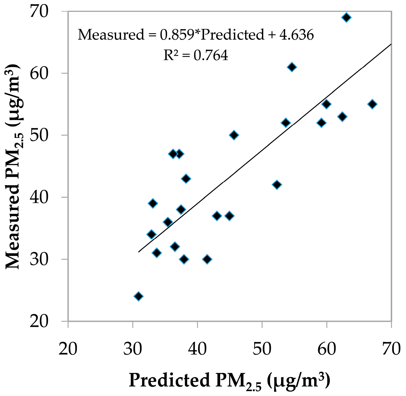
To evaluate the performance of the final LUR models, the equations were applied to the test data set and the R2 value between the predicted and measured PM2.5 concentrations was calculated. The R2 value was 0.764. In addition, predicted data were plotted against measured data for validation (Figure 2). The figure shows that the predicted PM2.5 concentrations were well correlated with the measured concentrations.
Grids with a dimension of 1 km 1 km were created in the whole study area and the seasonal PM2.5 concentrations were calculated at each intersection using the final LUR models. We assumed there was no trend in the data and a spatially homogenous variation, and the seasonal spatial distributions of PM2.5 were then interpolated using the Ordinary Kriging approach. As shown in Figure 3, PM2.5 concentrations demonstrated a discernible spatial variation. High concentration areas occurred in the centre of the study area, while low concentration areas were mainly distributed on city borders. The northwest and southwest were low concentration areas throughout the year. The figure also discloses that the PM2.5 concentrations of most of the Nanchang urban area met the legislated 24-h average value, but exceeded the annual mean value, which are 75 μg/m3 and 35 μg/m3 in China, respectively.
3.2. Statistic Analysis of PM2.5 ConcentrationVariances among Different Types of Urban Functional Zones
Five types and a total of 25 urban functional zones were selected in the study area to analyze the PM2.5 concentration variances among different types of urban functional zones, as shown in Figure 4. The PM2.5 concentrations in the four seasons of these functional zones are shown in Table 4.
Analyses of the PM2.5 concentration variances in the urban functional zones were conducted after a normal distribution test and variance homogeneity test. Table 5 shows the one-factor variance analysis results. In spring, the F-ratio of 18.062 (p < 0.01) indicates that the PM2.5 concentration variances among different types of urban functional zones were significant. We can also conclude the same rule in summer, autumn, and winter.
Table 4 also expresses the multiple comparison results. In the four seasons, the multiple comparison results among different types of urban functional zones were the same. The results show that the PM2.5 concentration variances between the control and other four types of urban functional zones were significant. The PM2.5 concentration variances between the industrial or commercial functional zones and the residential or educational functional zones were also significant. However, there were no statistically significant PM2.5 concentration variances between the industrial and commercial functional zones, and the educational and residential functional zones.
3.3. Statistic Analysis of PM2.5 Concentration Variances among the Same Type of Urban Functional Zones
Since residential land occupies the highest proportion of the urban area, the residential zone was selected as the typical functional zone to analyze PM2.5 concentration variances among the same type of urban functional zone. Another 15 residential functional zones were added to the original residential zone sample. Variables of intensity of the main roads, building volume rate, building density, and green coverage rate were used to build the multiple linear regression model for the annual PM2.5 prediction. As Table 6 shows, the model had a low fitting degree (adjusted R2 = 0.363). The intensity of the main roads positively correlated with PM2.5 concentrations and was the primary influencing variable in PM2.5 prediction (p < 0.01). The building volume rate was positively correlated with PM2.5 concentrations (p > 0.1) and the green coverage rate was negatively correlated with PM2.5 concentrations (p > 0.1). The building density showed a negative correlation with PM2.5 concentrations, which was counter-intuitive (p > 0.1).
4. Discussion
4.1. LUR Models
We developed LUR models incorporating meteorological factors for predicting quarterly PM2.5 concentrations in the Nanchang urban area, China. The adjusted R2 values of the seasonal LUR models were 0.764, 0.899, 0.941, 0.961, respectively, explaining the spatial variability of the pollutant concentrations. In previous studies, the adjusted R2 values of the LUR models ranged from 0.36 to 0.94 for PM2.5 [40,41]. The good performance of our models may be attributed to the combination of meteorological factors. Few LUR models include meteorological variables, although many studies have demonstrated that meteorology can significantly influence the pollutant concentration [23,24,25,26], possibly due to the lack of enough data or an appropriate methodology. Obtaining the meteorological conditions at each monitoring site is costly and time-consuming. In this study, we presupposed an identical meteorological condition at every site, as the study area was not very large. Different meteorological factors were entered into the LUR models of different seasons, demonstrating that the influence of meteorological factors on PM2.5 concentrations varied as the seasons changed.
Among all the independent variables, the intensity of main roads within a 300 m buffer was the dominant variable affecting PM2.5 concentrations, indicating that PM2.5 concentrations are closely related to traffic conditions. Some studies used vehicle intensity, while other studies used road length or road intensity to represent traffic conditions [26,42,43,44,45]. Compared to road length or road intensity, vehicle intensity is more representative of vehicle exhaust, but the data are often unavailable for researchers because of the high cost of vehicle monitoring. Studies have also proved that the performance of LUR models developed with road length or road intensity didn’t differ from those developed with vehicle intensity [35,46]. Therefore, road intensity was used in our models in the absence of vehicle intensity. The independent variable of industrial land proportion increasing PM2.5 pollution in other studies was also included in the LUR models [33,42]. The variables of road intensity and industrial land proportion implying sources of PM2.5 in Nanchang are mainly local transportation and major industries. The independent variable of ecological land proportion decreasing PM2.5 pollution in other Chinese cities was also included in the LUR models [33,47], suggesting that the function of natural spaces in removing pollutants is evident. It should be noticed that the independent variable of population density increasing PM2.5 concentration in other Chinese cities was not included in our models [33,47]. The reason for this is that the spatial resolution of the variable was not good enough in our study.
The number of monitoring sites might be an important factor influencing the accuracy of LUR models. However, at present, there is no rigorous methodology to determine the number of required monitoring sites. The population and size of cities are generally thought to be taken into account when determining the actual number of monitoring sites [40]. In our study, there were eight monitoring sites and the coverage area was 562.46 km2, resulting in a monitoring density of one site for every 70 km2. Although it was a small number of monitoring sites, the spatial coverage was comparable to other LUR models reported in the literature [33,35,37,42,46].
4.2. Impact of Land Use on PM2.5 Pollution
The paper studied the impact of land use on PM2.5 pollution from two aspects of land use type and land use intensity. The impact of land use type on PM2.5 pollution was investigated by analyzing the PM2.5 concentration variances among different types of urban functional zones. Through the analysis of PM2.5 data from different types of functional zones, the same rule in four seasons was found. The highest PM2.5 concentration was found in industrial and commercial functional zones, while the lowest occurred in control functional zones. The PM2.5 concentration in residential and educational functional zones was in between these zone types. PM2.5 pollution in the commercial zone was relatively high in comparison with industrial functional zones, and the residential zone was slightly higher than educational functional zones. The PM2.5 concentrations in different types of functional zones have also been investigated through a sample survey and a similar pattern has been found [48], which confirms the high simulation accuracy of the final LUR models. Further, our results demonstrate that the PM2.5 concentration variances among different urban functional zones were statistically significant. The significant PM2.5 variances suggest that the PM2.5 pollutants in the Nanchang urban area mainly come from local transportation and major industries, echoing the results demonstrated in the LUR models. We can also conclude that the urban functional zones which are characterized by a dominant land use type had a great impact on PM2.5 pollution and the impact did not change as the seasons changed.
The impact of land use intensity on PM2.5 pollution was investigated through predicting annual PM2.5 concentrations with indexes including the building volume rate, building density, and green coverage rate. The concept of land use intensity is far from an innovative term and first appeared in David Ricardo’s Land Rent Theory, which is similar to concepts of smart growth, compact city, Infill Development, and Urban Growth Boundary [49]. In China, land use intensity is considered as the national guideline to alleviate the demand for urban land driven by economic and population growth. However, studies have shown that a higher land use intensity leads to more prominent environmental problems, like noise, dust, and toxic pollutants, because a higher land use intensity increases the concentration of the urban activities [50]. In our paper, the multiple linear regression results showed insignificant t-statistics and inconsistent coefficients with a priori assumptions, illustrating that the indexes had an insignificant or counter-intuitive impact on PM2.5 concentrations. This may due to the complex physical-chemical mechanism of PM2.5 pollution or the improper study spatial scale.
In our paper, urban functional zones were used as the basic research unit to explore the effect of land use on PM2.5 pollution. Some studies analyzed the effect of land use on PM2.5 pollution through calculating the correlation between PM2.5 pollution and land use/land cover types [34,51,52]. Compared to a single land use type, urban functional zones including a variety of land use types, but characterized by a dominant land use type, are more appropriate for urban areas. Scholars also believe that urban functional zones can better reflect the relationship between urban land use and air pollution as its specific social-economic function [30]. The results demonstrate that the urban functional zone was a proper spatial scale to investigate the impact of land use type on PM2.5 pollution in urban areas.
4.3. Limitations
There are some limitations that need to be addressed. The first limitation of this study was the weakness related to applying the LUR model to a large area. As the study area in our paper is not very large, we presupposed identical meteorological conditions at every monitoring site. In large areas, the meteorological variables vary from one monitoring site to another and will show a differential influence at each site. Secondly, only a one-year period was considered in this paper due to the data access limitations. Using data from longer periods can help improve the prediction ability of an LUR model. Lastly, it should be noted that this research has explored the impact of land use on PM2.5 pollution through analyzing the intra-urban spatial variability of PM2.5 concentrations. Further research is needed to investigate the detailed mechanisms of how land use influences PM2.5 concentration.
5. Conclusions
This paper attempted to use LUR models to simulate the variances of the PM2.5 level in the Nanchang urban area and statistical analysis to explore the impact of land use on PM2.5 pollution. The seasonal LUR models showed a good fit and could explain the spatial variability in PM2.5 concentrations well. PM2.5 exhibits a large variation in different seasons, with the highest pollution values in winter and the lowest in summer, due to the complicated influence of the meteorological factors of temperature and relative humidity [53,54]. Similar to many other studies, the dominant PM2.5 impacting variable was the traffic conditions that were characterized by the road intensity in this paper [37,42,55,56,57]. The analysis of variance and multiple comparison test shows statistically significant variances in PM2.5 concentrations among different types of urban functional zones throughout the year, demonstrating that the land use types generated a great impact on PM2.5 concentrations and the impact did not change as the seasons changed. The multiple linear regression results illustrate that the land use intensity indexes including the building volume rate, building density, and green coverage rate exhibited an insignificant or counter-intuitive impact on PM2.5 concentrations. The study also concludes that the urban functional zone was a proper spatial scale to investigate the impact of land use type on PM2.5 pollution in urban areas, but might not be a proper spatial scale to explore the impact of land use intensity on PM2.5 pollution. A reasonable methodology and optimized spatial scale are still yet to be explored to further investigate how land use intensity affects PM2.5 pollution.
Acknowledgments
This research was funded by the Natural Science Foundation of China (No. 41561043). The authors greatly appreciate the thorough review and valuable comments of the anonymous reviewer that helped improve this manuscript.
Author Contributions
The study was designed and written by Haiou Yang and Wenbo Chen. Zhaofeng Liang was responsible for data collecting and analysis. The results were analyzed by Haiou Yang and Wenbo Chen.
Conflicts of Interest
The authors declare no conflict of interest.
References
- Han, L.; Zhou, W.; Li, W.; Li, L. Impact of urbanization level on urban air quality: A case of fine particles (PM2.5) in Chinese cities. Environ. Pollut. 2014, 194, 163–170. [Google Scholar] [CrossRef] [PubMed]
- Makkonen, U.; Hellén, H.; Anttila, P.; Ferm, M. Size distribution and chemical composition of airborne particles in south-eastern Finland during different seasons and wildfire episodes in 2006. Sci. Total Environ. 2010, 408, 644–651. [Google Scholar] [CrossRef] [PubMed]
- Pope, C.A., III; Dockery, D.W. Health effects of fine particulate air pollution: Lines that connect. J. Air Waste Manag. 2006, 56, 709–742. [Google Scholar] [CrossRef]
- Pope, C.A.; Turner, M.C.; Burnett, R.; Jerrett, M.; Gapstur, S.M.; Diver, W.R.; Krewski, D.; Brook, R.D. Relationships between fine particulate air pollution, cardiometabolic disorders, and cardiovascular mortality. Circ. Res. 2015, 116, 108–115. [Google Scholar] [CrossRef] [PubMed]
- Eeftens, M.; Tsai, M.-Y.; Ampe, C.; Ampe, C.; Anwander, B.; Beelen, R.; Bellander, T.; Cesaroni, G.; Cirach, M.; Cyrys, J.; et al. Spatial variation of PM2.5, PM10, PM2.5 absorbance and PM coarse concentrations between and within 20 European study areas and the relationship with NO2–results of the ESCAPE project. Atmos. Environ. 2012, 62, 303–317. [Google Scholar] [CrossRef]
- Querol, X.; Alastuey, A.; Moreno, T.; Viana, M.M.; Castillo, S. Spatial and temporal variations in airborne particulate matter (PM10 and PM2.5) across Spain 1999–2005. Atmos. Environ. 2008, 42, 3964–3979. [Google Scholar] [CrossRef]
- Lin, G.; Fu, J.; Jiang, D.; Hu, W.; Dong, D.; Huang, Y.; Zhao, M. Spatio-temporal variation of PM2.5 concentrations and their relationship with geographic and socioeconomic factors in China. Int. J. Environ. Res. Public Health 2013, 11, 173–186. [Google Scholar] [CrossRef] [PubMed]
- Chen, T.; He, J.; Lu, X.; She, J.; Guan, Z. Spatial and temporal variations of PM2.5 and its relation to meteorological factors in the urban area of Nanjing, China. Int. J. Environ. Res. Public Health 2016, 13, 921. [Google Scholar] [CrossRef] [PubMed]
- Wang, Y.G.; Ying, Q.; Hu, J.L.; Zhang, H.L. Spatial and temporal variations of six criteria air pollutants in 31 provincial capital cities in China during 2013–2014. Environ. Int. 2014, 73, 413–422. [Google Scholar] [CrossRef] [PubMed]
- Zhang, H.; Wang, Z.; Zhang, W. Exploring spatiotemporal patterns of PM2.5 in China based on ground-level observations for 190 cities. Environ. Pollut. 2016, 216, 559–567. [Google Scholar] [CrossRef] [PubMed]
- Behera, S.N.; Sharma, M. Reconstructing primary and secondary components of PM2.5 composition for an urban atmosphere. Aerosol Sci. Technol. 2010, 44, 983–992. [Google Scholar] [CrossRef]
- Wang, Z.; Hu, M.; Wu, Z.; Yue, D.; He, L.; Huang, X.; Liu, X.; Wiedensohler, A. Long-term measurements of particle number size distributions and the relationships with air mass history and source apportionment in the summer of Beijing. Atmos. Chem. Phys. 2013, 13, 10159–10170. [Google Scholar] [CrossRef]
- Wu, D.W.; Fung, J.C.; Yao, T.; Lau, A.K. A study of control policy in the Pearl River Delta region by using the particulate matter source apportionment method. Atmos. Environ. 2013, 76, 147–161. [Google Scholar] [CrossRef]
- Wang, Y.; Li, L.; Chen, C.; Huang, C.; Huang, H.; Feng, J.; Wang, S.; Wang, H.; Zhang, G.; Zhou, M.; et al. Source apportionment of fine particulate matter during autumn haze episodes in Shanghai, China. J. Geophys. Res. 2014, 119, 1903–1914. [Google Scholar] [CrossRef]
- Brook, R.D.; Rajagopalan, S.; Pope, C.A.; Brook, J.R.; Bhatnagar, A.; Diez-Roux, A.V.; Holguin, F.; Hong, Y.; Luepker, R.V.; Mittleman, M.A. Particulate matter air pollution and cardiovascular disease an update to the scientific statement from the American Heart Association. Circulation 2010, 121, 2331–2378. [Google Scholar] [CrossRef] [PubMed]
- Bell, M.L. Assessment of the Health Impacts of Particulate Matter Characteristics; Research Report, No 161; Health Effects Institute: Boston, MA, USA, 2012; pp. 5–38. [Google Scholar]
- Fann, N.; Lamson, A.D.; Anenberg, S.C.; Wesson, K.; Risley, D.; Hubbell, B.J. Estimating the national public health burden associated with exposure to ambient PM2.5 and ozone. Risk Anal. 2012, 32, 81–95. [Google Scholar] [CrossRef] [PubMed]
- Kim, S.Y.; Peel, J.L.; Hannigan, M.P.; Dutton, S.J.; Sheppard, L.; Clark, M.L.; Vedal, S. The temporal lag structure of short-term associations of fine particulate matter chemical constituents and cardiovascular and respiratory hospitalizations. Environ. Health Perspect. 2012, 120, 1094. [Google Scholar] [CrossRef] [PubMed]
- Beckerman, B.S.; Jerrett, M.; Serre, M.; Martin, R.V.; Lee, S.-J.; van Donkelaar, A.; Ross, Z.; Su, J.; Burnett, R.T. A hybrid approach to estimating national scale spatiotemporal variability of PM2.5 in the contiguous United States. Environ. Sci. Technol. 2013, 47, 7233–7241. [Google Scholar] [PubMed]
- Geng, G.; Zhang, Q.; Martin, R.V.; van Donkelaar, A.; Huo, H.; Che, H.; Lin, J.; He, K. Estimating long-term PM2.5 concentrations in China using satellite-based aerosol optical depth and a chemical transport model. Remote Sens. Environ. 2015, 166, 262–270. [Google Scholar] [CrossRef]
- Just, A.C.; Wright, R.O.; Schwartz, J.; Coull, B.A.; Baccarelli, A.A.; Tellez-Rojo, M.M.; Moody, E.; Wang, Y.; Lyapustin, A.; Kloog, I. Using high-resolution satellite aerosol optical depth to estimate daily PM2.5 geographical distribution in Mexico City. Environ. Sci. Technol. 2015, 49, 8576–8584. [Google Scholar] [CrossRef] [PubMed]
- Zhang, T.; Gong, W.; Wang, W.; Ji, Y.; Zhu, Z.; Huang, Y. Ground level PM2.5 estimates over China using satellite-based geographically weighted regression (GWR) models are improved by including NO2 and enhanced vegetation index (EVI). Int. J. Environ. Res. Public Health 2016, 13, 1215. [Google Scholar] [CrossRef] [PubMed]
- Arain, M.A.; Blair, R.; Finkelstein, N.; Brook, J.R.; Sahsuvaroglu, T.; Beckerman, B.; Zhang, L.; Jerrett, M. The use of wind fields in a land use regression model to predict air pollution concentrations for health exposure studies. Atmos. Environ. 2007, 41, 3453–3464. [Google Scholar] [CrossRef]
- Madsen, C.; Carlsen, K.C.L.; Hoek, G.; Oftedal, B.; Nafstad, P.; Meliefste, K.; Jacobsen, R.; Nystad, W.; Carlsen, K.-H.; Brunekreef, B. Modeling the intra-urban variability of outdoor traffic pollution in Oslo, Norway—A GA 2 LEN project. Atmos. Environ. 2007, 41, 7500–7511. [Google Scholar] [CrossRef]
- Wilton, D.; Szpiro, A.; Gould, T.; Larson, T. Improving spatial concentration estimates for nitrogen oxides using a hybrid meteorological dispersion/land use regression model in Los Angeles, CA and Seattle, WA. Sci. Total Environ. 2010, 408, 1120–1130. [Google Scholar] [CrossRef] [PubMed]
- Li, X.; Liu, W.; Chen, Z.; Zeng, G.; Hu, C.; León, T.; Liang, J.; Huang, G.; Gao, Z.; Li, Z.; et al. The application of semicircular-buffer-based land use regression models incorporating wind direction in predicting quarterly NO2 and PM10 concentrations. Atmos. Environ. 2015, 103, 18–24. [Google Scholar] [CrossRef]
- Lam, T.; Niemeier, D. An exploratory study of the impact of common land-use policies on air quality. Transp. Res. D-Transp. Environ. 2005, 10, 365–383. [Google Scholar] [CrossRef]
- Bandeira, J.M.; Coelho, M.C.; Sá, M.E.; Tavares, R.; Borrego, C. Impact of land use on urban mobility patterns, emissions and air quality in a Portuguese medium-sized city. Sci. Total Environ. 2011, 409, 1154–1163. [Google Scholar] [CrossRef] [PubMed]
- Zhang, R.S.; Pu, L.J.; Liu, Z. Advances in research on atmospheric environment effects of land use and land cover change. Area Res. Dev. 2013, 32, 123–128. [Google Scholar]
- Chen, L.D.; Sun, R.H.; Liu, H.L. Eco-environmental effects of urban landscape pattern changes: Progresses, problems and perspectives. Acta Ecol. Sin. 2013, 33, 1042–1050. [Google Scholar] [CrossRef]
- Briggs, D.J.; de Hoogh, C.; Gulliver, J.; Wills, J.; Elliott, P.; Kingham, S.; Smallbone, K. A regression-based method for mapping traffic-related air pollution: Application and testing in four contrasting urban environments. Sci. Total Environ. 2000, 253, 151–167. [Google Scholar] [CrossRef]
- Jerrett, M.; Arain, A.; Kanaroglou, P.; Beckerman, B.; Potoglou, D.; Sahsuvaroglu, T.; Morrison, J.; Giovis, C. A review and evaluation of intra-urban air pollution exposure models. J. Expo. Sci. Environ. Epidemiol. 2005, 15, 185–204. [Google Scholar] [CrossRef] [PubMed]
- Liu, C.; Henderson, B.H.; Wang, D.; Yang, X.; Peng, Z.-R. A land use regression application into assessing spatial variation of intra-urban fine particulate matter (PM2.5) and nitrogen dioxide (NO2) concentrations in City of Shanghai, China. Sci. Total Environ. 2016, 565, 607–615. [Google Scholar] [CrossRef] [PubMed]
- Sun, L.; Wei, J.; Duan, D.H.; Guo, Y.M.; Yang, D.X.; Jia, C.; Mi, X.T. Impact of Land-Use and Land-Cover Change on urban air quality in representative cities of China. J. Atmos. Sol.-Terr. Phys. 2016, 142, 43–54. [Google Scholar] [CrossRef]
- Henderson, S.B.; Beckerman, B.; Jerrett, M.; Brauer, M. Application of land use regression to estimate long-term concentrations of traffic-related nitrogen oxides and fine particulate matter. Environ. Sci. Technol. 2007, 41, 2422–2428. [Google Scholar] [CrossRef] [PubMed]
- Liu, W.; Li, X.; Chen, Z.; Zeng, G.; León, T.; Liang, J.; Huang, G.; Gao, Z.; Jiao, S.; He, X.; et al. Land use regression models coupled with meteorology to model spatial and temporal variability of NO2, and PM10, in Changsha, China. Atmos. Environ. 2015, 116, 272–280. [Google Scholar] [CrossRef]
- Olvera, H.A.; Garcia, M.; Li, W.-W.; Yang, H.; Amaya, M.A.; Myers., O.; Burchiel, S.W.; Berwick, M.; Pingitore, N.E., Jr. Principal component analysis optimization of a PM2.5 land use regression model with small monitoring network. Sci. Total Environ. 2012, 425, 27–34. [Google Scholar] [CrossRef] [PubMed]
- Briggs, D.J.; Collins, S.; Elliott, P.; Fischer, P.; Kingham, S.; Lebret, E.; Pryl, K.; Reeuwijk, H.V.; Smallbone, K.; Van Der Veen, A. Mapping urban air pollution using GIS: A regression-based approach. Int. J. Geogr. Inf. Sci. 1997, 11, 699–718. [Google Scholar] [CrossRef]
- Hogg, R.V.; Ledolter, J. Engineering Statistics; Macmillan Pub. Co.: New York, NY, USA, 1987. [Google Scholar]
- Hoek, G.; Beelen, R.; De Hoogh, K.; Vienneau, D.; Gulliver, J.; Fischer, P.; Briggs, D. A review of land-use regression models to assess spatial variation of outdoor air pollution. Atmos. Environ. 2008, 42, 7561–7578. [Google Scholar] [CrossRef]
- Eeftens, M.; Beelen, R.; de Hoogh, K.; Bellander, T.; Cesaroni, G.; Cirach, M.; Declercq, C.; Dedele, A.; Dons, E.; de Nazelle, A.; et al. Development of land use regression models for PM2.5, PM2.5 absorbance, PM10 and PM coarse in 20 European study areas; results of the ESCAPE project. Environ. Sci. Technol. 2012, 46, 11195–11205. [Google Scholar] [CrossRef] [PubMed]
- Ross, Z.; Jerrett, M.; Ito, K.; Tempalski, B.; Thurston, G.D. A land use regression for predicting fine particulate matter concentrations in the New York City region. Atmos. Environ. 2007, 41, 2255–2269. [Google Scholar] [CrossRef]
- Hochadel, M.; Heinrich, J.; Gehring, U.; Morgenstern, V.; Kuhlbusch, T.; Link, E.; Wichmann, H.-E.; Krämer, U. Predicting long-term average concentrations of traffic-related air pollutants using GIS-based information. Atmos. Environ. 2006, 40, 542–553. [Google Scholar] [CrossRef]
- Beelen, R.; Hoek, G.; Vienneau, D.; Eeftens, M.; Dimakopoulou, K.; Pedeli, X.; Tsai, M.-Y.; Künzli, N.; Schikowski, T.; Marcon, A. Development of NO2 and NOx land use regression models for estimating air pollution exposure in 36 study areas in Europe—The ESCAPE project. Atmos. Environ. 2013, 72, 10–23. [Google Scholar] [CrossRef]
- Wang, R.; Henderson, S.B.; Sbihi, H.; Allen, R.W.; Brauer, M. Temporal stability of land use regression models for traffic-related air pollution. Atmos. Environ. 2013, 64, 312–319. [Google Scholar] [CrossRef]
- Lee, J.-H.; Wu, C.-F.; Hoek, G.; de Hoogh, K.; Beelen, R.; Brunekreef, B.; Chan, C.-C. Land use regression models for estimating individual NOx and NO2 exposures in a metropolis with a high density of traffic roads and population. Sci. Total Environ. 2014, 472, 1163–1171. [Google Scholar] [CrossRef] [PubMed]
- Wu, J.; Li, J.; Peng, J.; Li, W.; Xu, G.; Dong, C. Applying land use regression model to estimate spatial variation of PM2.5 in Beijing, China. Environ. Sci. Pollut. Res. 2015, 22, 7045–7061. [Google Scholar] [CrossRef] [PubMed]
- He, Z.J.; Yuan, S.L.; Xiao, M. Pollution levels of airborne particulate matter PM10 and PM2.5 in summer in Nanchang City. J. Anhui Agric. Sci. 2009, 38, 1336–1338. [Google Scholar]
- Huang, D.Q.; Wan, W.; Dai, T.Q.; Liang, J.S. Assessment of industrial land use intensity: A case study of Beijing Economic-technological Development Area. Chin. Geogr. Sci. 2011, 21, 222–229. [Google Scholar] [CrossRef]
- Carsjens, G.J.; Ligtenberg, A. A GIS-based support tool for sustainable spatial planning in metropolitan areas. Landsc. Urban Plan. 2007, 80, 72–83. [Google Scholar] [CrossRef]
- Wei, J.; Sun, L.; Liu, S.S. Response analysis of particulate air pollution to land-use and land-cover. Acta Ecol. Sin. 2015, 35, 5495–5506. [Google Scholar]
- Tang, X.M.; Liu, H.; Li, J. Response analysis of haze/particulate matter pollution to land use/cover in Beijing. China Environ. Sci. 2015, 35, 2561–2569. [Google Scholar]
- Chen, X.X.; Hu, L.; Peng, W.M.Z.; Liu, B. Characteristics of meteorological parameters and main atmospheric pollutants of haze events in Nanchang from 1960 to 2014. J. Meteor. Environ. 2016, 2, 114–121. [Google Scholar]
- Su, W.; Zhang, S.J.; Lai, X.Y.; Gu, X.R.; Lai, S.N; Huang, G.X.; Zhang, Z.J.; Liu, Y.Q. Spatiotemporal dynamics of atmospheric PM2.5 and PM10 and its influencing factors in Nanchang, China. Chin. J. Appl. Ecol. 2017, 28, 257–265. [Google Scholar]
- Moore, D.K.; Jerrett, M.; Mack, W.J.; Künzli, N. A land use regression model for predicting ambient fine particulate matter across Los Angeles, CA. J. Environ. Monit. 2007, 9, 246–252. [Google Scholar] [CrossRef] [PubMed]
- Ryan, P.H.; Lemasters, G.K. A review of land-use regression models for characterizing intra-urban air pollution exposure. Inhal. Toxicol. 2007, 19, 127–133. [Google Scholar] [CrossRef] [PubMed]
- Lee, J.H.; Wu, C.F.; Hoek, G.; de Hoogh, K.; Beelen, R.; Brunekreef, B.; Chan, C.C. LUR models for particulate matters in the Taipei metropolis with high densities of roads and strong activities of industry, commerce and construction. Sci. Total Environ. 2015, 514, 178–184. [Google Scholar] [CrossRef] [PubMed]
Figure 1.
Map of the Nanchang urban area showing the monitoring site locations and road network.
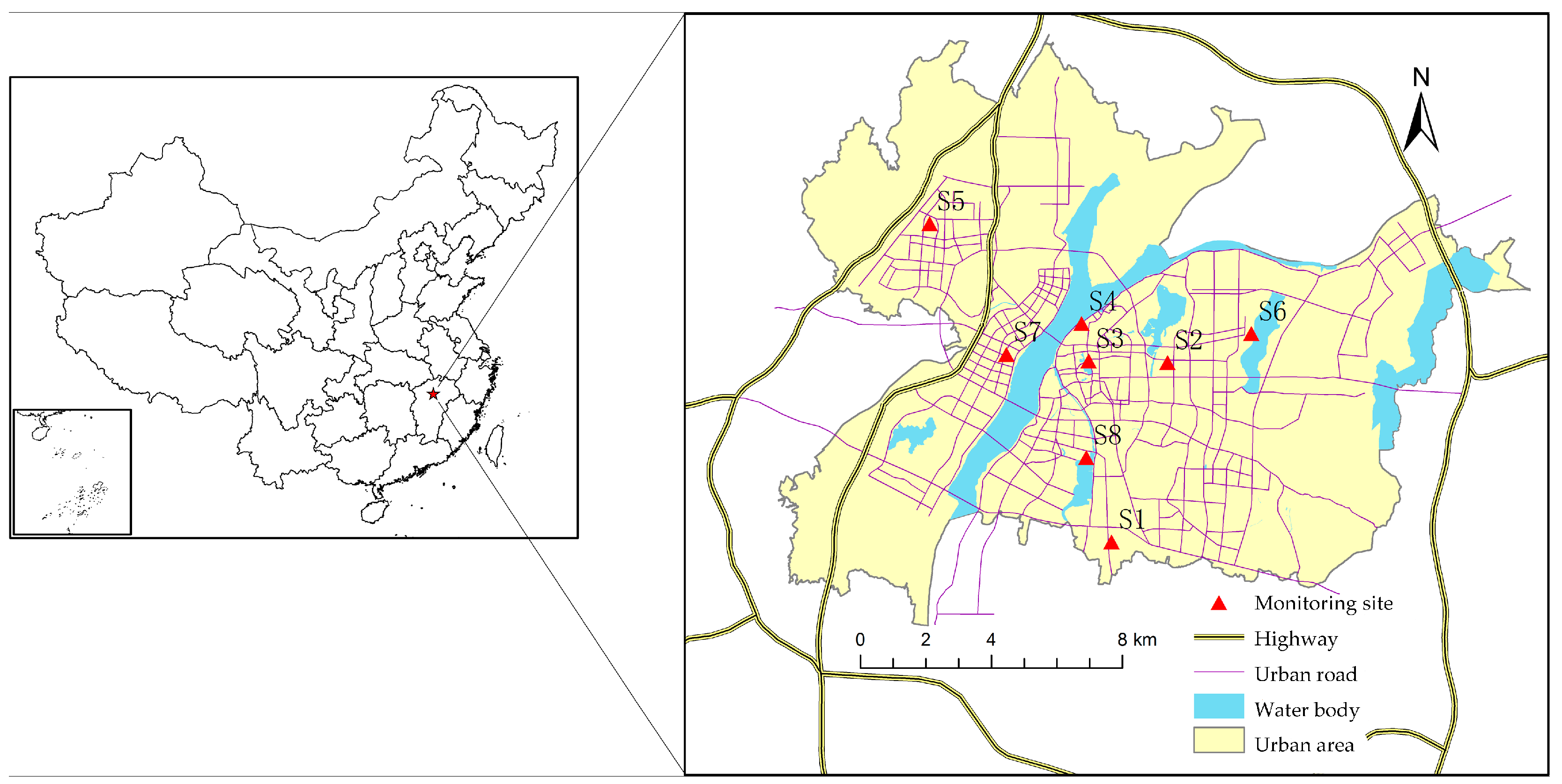
Figure 2.
Predicted versus measured PM2.5 concentrations of the test data set.

Figure 3.
Final LUR models applied in the Nanchang urban area: PM2.5 concentrations in (a) Spring; (b) Summer; (c) Autumn; (d) Winter.
Figure 3.
Final LUR models applied in the Nanchang urban area: PM2.5 concentrations in (a) Spring; (b) Summer; (c) Autumn; (d) Winter.
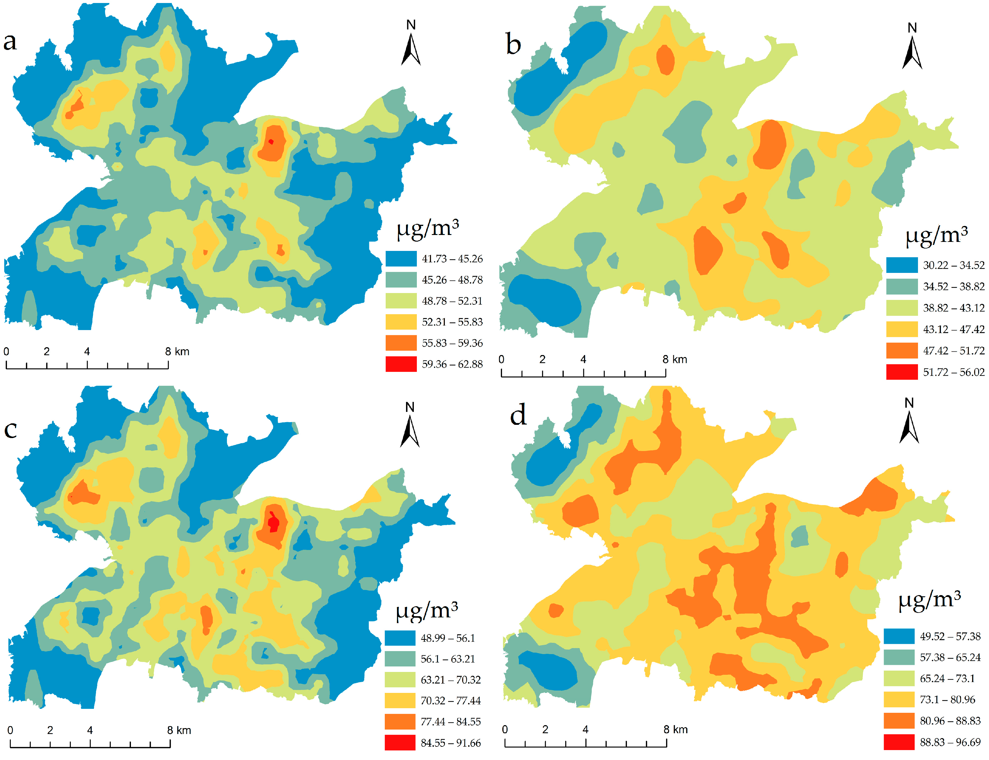
Figure 4.
Location map of the urban functional zones in the Nanchang urban area.


Table 1.
The time-serial fine particulate matter (PM2.5) concentrations for the eight monitoring sites in 2014.
Table 1.
The time-serial fine particulate matter (PM2.5) concentrations for the eight monitoring sites in 2014.
| Monitoring Site | Month (μg/m3) | |||||||||||
|---|---|---|---|---|---|---|---|---|---|---|---|---|
| Jan. | Feb. | Mar. | Apr. | May | Jun. | Jul. | Aug. | Sep. | Oct. | Nov. | Dec. | |
| S1 | 105 | 38 | 46 | 45 | 61 | 50 | 36 | 34 | 52 | 92 | 74 | 61 |
| S2 | 109 | 38 | 44 | 37 | 45 | 39 | 27 | 25 | 36 | 67 | 54 | 52 |
| S3 | 119 | 41 | 45 | 48 | 71 | 55 | 38 | 38 | 57 | 92 | 62 | 55 |
| S4 | 102 | 37 | 44 | 47 | 69 | 55 | 36 | 37 | 52 | 92 | 61 | 54 |
| S5 | 88 | 27 | 36 | 30 | 42 | 39 | 27 | 24 | 35 | 58 | 38 | 38 |
| S6 | 97 | 32 | 36 | 37 | 60 | 47 | 33 | 31 | 44 | 81 | 55 | 51 |
| S7 | 96 | 39 | 47 | 40 | 48 | 46 | 42 | 34 | 38 | 53 | 50 | 36 |
| S8 | 87 | 30 | 37 | 39 | 49 | 55 | 47 | 43 | 59 | 81 | 60 | 57 |
Table 2.
The description of independent variables.
| Variable | Unit | Max | Min | Mean | SD |
|---|---|---|---|---|---|
| Relative humidity | % | 80 | 57 | 74.167 | 8.077 |
| Air pressure | hpa | 1022.3 | 998.8 | 1009.750 | 7.994 |
| Water vapor pressure | hpa | 31.8 | 5.8 | 18.075 | 9.167 |
| Temperature | °C | 29 | 7.3 | 18.817 | 8.183 |
| Wind speed | m/s | 1.9 | 1.4 | 1.675 | 0.166 |
| Intensity of main roads (300–4800 m) | m/m2 | 0.270 | 0 | 0.113 | 0.061 |
| Intensity of secondary roads (300–4800 m) | m/m2 | 0.428 | 0 | 0.085 | 0.100 |
| Intensity of total roads (300–4800 m) | m/m2 | 0.644 | 0 | 0.220 | 0.115 |
| Ecological land proportion (300–4800 m) | % | 99.728 | 5.483 | 39.027 | 20.233 |
| Industrial land proportion (300–4800 m) | % | 53.515 | 0 | 11.433 | 14.699 |
| Distance to large ecological space | m | 1826 | 67 | 827.500 | 659.948 |
| Residential land proportion (300–4800 m) | % | 49.015 | 0 | 18.438 | 11.973 |
Note: SD means standard deviation.
Table 3.
The final land use regression (LUR) models for PM2.5 concentrations in the Nanchang urban area.
Table 3.
The final land use regression (LUR) models for PM2.5 concentrations in the Nanchang urban area.
| Season | Model Variable | β | SE | p | VIF | Adj. R2 | SE |
|---|---|---|---|---|---|---|---|
| Spring | Intercept | 46.722 | 1.050 | 0.000 | 0.764 | 4.455 | |
| Intensity of main roads (300 m) | 4.859 | 1.085 | 0.001 | 1.009 | |||
| Industrial land proportion (300 m) | 2.087 | 1.110 | 0.083 | 1.055 | |||
| Temperature | 16.748 | 3.061 | 0.000 | 8.023 | |||
| Relative Humidity | 11.521 | 3.049 | 0.002 | 7.963 | |||
| Summer | Intercept | 40.056 | 0.718 | 0.000 | 0.899 | 3.044 | |
| Intensity of main roads (300 m) | 3.008 | 0.763 | 0.002 | 1.067 | |||
| Industrial land proportion (300 m) | 3.103 | 0.858 | 0.054 | 1.351 | |||
| Ecological land proportion (2400 m) | −3.159 | 0.925 | 0.058 | 1.570 | |||
| Relative Humidity | −6.846 | 0.775 | 0.000 | 1.102 | |||
| Autumn | Intercept | 62.000 | 1.044 | 0.000 | 0.941 | 4.429 | |
| Intensity of main roads (300 m) | 9.469 | 1.149 | 0.000 | 1.143 | |||
| Industrial land proportion (300 m) | 3.213 | 1.147 | 0.056 | 1.141 | |||
| Ecological land proportion (300 m) | −2.825 | 1.199 | 0.058 | 1.247 | |||
| Relative Humidity | −14.150 | 1.156 | 0.000 | 1.159 | |||
| Winter | Intercept | 67.778 | 1.461 | 0.000 | 0.961 | 6.198 | |
| Intensity of main roads (300 m) | 4.805 | 1.541 | 0.008 | 1.051 | |||
| Distance to large ecological space | 3.380 | 1.690 | 0.067 | 1.264 | |||
| Ecological land proportion (2400 m) | −4.362 | 1.723 | 0.020 | 1.313 | |||
| Temperature | 30.048 | 1.513 | 0.000 | 1.014 |
Note: β is the associated coefficient of the LUR model, VIF means variance inflation factors.
Table 4.
PM2.5 concentrations in the functional zones in four seasons.
| Functional Zone Type | Mean ± SD/(μg·m−3) | |||
|---|---|---|---|---|
| Spring | Summer | Autumn | Winter | |
| Commercial zones | 53.396 ± 1.23a | 44.476 ± 0.89a | 75.062 ± 2.48a | 82.702 ± 1.37a |
| Industrial zones | 51.734 ± 1.11a | 43.272 ± 0.81a | 71.724 ± 2.23a | 80.856 ± 1.23a |
| Educational zones | 46.674 ± 0.95b | 39.806 ± 0.64b | 61.402 ± 1.98b | 65.498 ± 3.23b |
| Residential zones | 47.914 ± 1.16b | 40.502 ± 0.84b | 64.056 ± 2.32b | 68.624 ± 1.28b |
| Control zones | 42.500 ± 0.37c | 36.574 ± 0.27c | 53.174 ± 0.74c | 58.842 ± 0.34c |
Note: Different lowercase letters in the same column indicate significantly different PM2.5 concentrations in functional zones of the same season at 5%.
Table 5.
Variance analysis results.
| Season | Variable | Squares Sum | Freedom | Mean Square | F-Ratio | p-Value |
|---|---|---|---|---|---|---|
| Spring | Between-group | 370.695 | 4 | 92.674 | 18.062 | 0 |
| Within-group | 102.616 | 20 | 5.131 | |||
| Total | 473.31 | 24 | ||||
| Summer | Between-group | 192.401 | 4 | 48.1 | 18.264 | 0 |
| Within-group | 52.673 | 20 | 2.634 | |||
| Total | 245.074 | 24 | ||||
| Autumn | Between-group | 1500.56 | 4 | 375.14 | 17.888 | 0 |
| Within-group | 419.443 | 20 | 20.972 | |||
| Total | 1920.004 | 24 | ||||
| Winter | Between-group | 313.688 | 4 | 78.422 | 18.259 | 0 |
| Within-group | 85.901 | 20 | 4.295 | |||
| Total | 399.589 | 24 |
Table 6.
Multiple linear regression model for annual PM2.5 concentrations in residential zones.
| Model Variable | β | SE | p-Value | VIF | Adj. R2 | SE |
|---|---|---|---|---|---|---|
| Intercept | 52.178 | 4.059 | 0 | 0.363 | 4.707 | |
| Intensity of main roads (300 m) | 56.197 | 16.236 | 0.003 | 1.425 | ||
| Building volume rate | 0.577 | 0.996 | 0.555 | 2.308 | ||
| Building density | −0.016 | 0.059 | 0.785 | 1.991 | ||
| Green coverage rate | −0.181 | 0.162 | 0.281 | 1.636 |
© 2017 by the authors. Licensee MDPI, Basel, Switzerland. This article is an open access article distributed under the terms and conditions of the Creative Commons Attribution (CC BY) license (http://creativecommons.org/licenses/by/4.0/).
Share and Cite
MDPI and ACS Style
Yang, H.; Chen, W.; Liang, Z. Impact of Land Use on PM2.5 Pollution in a Representative City of Middle China. Int. J. Environ. Res. Public Health 2017, 14, 462. https://doi.org/10.3390/ijerph14050462
AMA Style
Yang H, Chen W, Liang Z. Impact of Land Use on PM2.5 Pollution in a Representative City of Middle China. International Journal of Environmental Research and Public Health. 2017; 14(5):462. https://doi.org/10.3390/ijerph14050462
Chicago/Turabian StyleYang, Haiou, Wenbo Chen, and Zhaofeng Liang. 2017. "Impact of Land Use on PM2.5 Pollution in a Representative City of Middle China" International Journal of Environmental Research and Public Health 14, no. 5: 462. https://doi.org/10.3390/ijerph14050462
Note that from the first issue of 2016, this journal uses article numbers instead of page numbers. See further details here.