Evaluation of the AnnAGNPS Model for Predicting Runoff and Nutrient Export in a Typical Small Watershed in the Hilly Region of Taihu Lake

Abstract

The application of hydrological and water quality models is an efficient approach to better understand the processes of environmental deterioration. This study evaluated the ability of the Annualized Agricultural Non-Point Source (AnnAGNPS) model to predict runoff, total nitrogen (TN) and total phosphorus (TP) loading in a typical small watershed of a hilly region near Taihu Lake, China. Runoff was calibrated and validated at both an annual and monthly scale, and parameter sensitivity analysis was performed for TN and TP before the two water quality components were calibrated. The results showed that the model satisfactorily simulated runoff at annual and monthly scales, both during calibration and validation processes. Additionally, results of parameter sensitivity analysis showed that the parameters Fertilizer rate, Fertilizer organic, Canopy cover and Fertilizer inorganic were more sensitive to TN output. In terms of TP, the parameters Residue mass ratio, Fertilizer rate, Fertilizer inorganic and Canopy cover were the most sensitive. Based on these sensitive parameters, calibration was performed. TN loading produced satisfactory results for both the calibration and validation processes, whereas the performance of TP loading was slightly poor. The simulation results showed that AnnAGNPS has the potential to be used as a valuable tool for the planning and management of watersheds.

1. Introduction

Non-point source pollution occurs when rainfall or irrigation water runs over land or through the ground, picks up pollutants and deposits them into rivers, lakes, or coastal waters or introduces them into ground water [1]. It is an important environmental and water quality management problem, and non-point sources presently account for the majority of water quality problems [2]. The increases in nutrient losses and riverine nutrient loads have resulted in nuisance algal blooms, the depletion of dissolved oxygen, and other water quality impairments [3]. Severe problems with water quality seem to make it unlikely that the water body will continue to support aquatic life and human consumption [4].

Watershed modeling can be a valuable tool for studying the relationships between conditions and the quality of water in a watershed [5]. The modeling of environmental deterioration to better understand and manage natural resources, such as river basins and watersheds, is a continuous process. Basin scale models that incorporate weather data and watershed characteristics such as topography assist in the delineation of the watershed and are tools for the development of management strategies in a watershed and river basins [6]. In the last four decades, several hydrological and water quality models have been developed to assist in understanding hydrologic systems and pollutant loadings [7], such as AnnAGNPS (Annualized Agricultural Non-Point Source Pollution Model) [8], ANSWERS (Areal Non-point Source Watershed Environment Response Simulation) [9], SWAT (Soil and Water Assessment Tool) [10], and HSPF (Hydrological Simulation Program FORTRAN) [11]. These models can be used to simulate the transport processes of runoff, sediment, nutrients and other chemical substances. Detailed reviews of these models can be found in the literature [12,13,14].

The AnnAGNPS model combines the latest advances in GIS (Geographic Information System) data manipulation with physical characterization of the catchments, offering modeling opportunities for ungauged areas or for areas with limited data that prohibit the use of models relying on calibration for the derivation of input variables [15]. The model has been successfully used in many areas of the world in recent years, including Spain [16,17,18], Nepal [19], Italy [20], Canada [21], USA [22,23,24] and China [5]. These studies evaluated the ability of the AnnAGNPS model to predict runoff and pollutant loadings under different climate or land-use conditions in various watersheds with areas ranging from 0.1 to 130 km². However, many of those studies have focused on evaluating the model’s suitability and on testing its performance regarding hydrologic and sediment transport estimation [16,17,18,19,20,21,22,23,24], and few efforts have been made to analyze the sensitive parameters for nutrient concentrations and to evaluate the model’s ability to predict them [4,15,25,26]. Thus, the purpose of this study is to validate the capability of the AnnAGNPS model to predict runoff and to analyze the sensitive parameters in regard to nutrient concentrations and evaluate the capability of the model to simulate nutrient loadings in a small watershed for a long time period (nine years).

2. Materials and Methods

2.1. AnnAGNPS Model Description

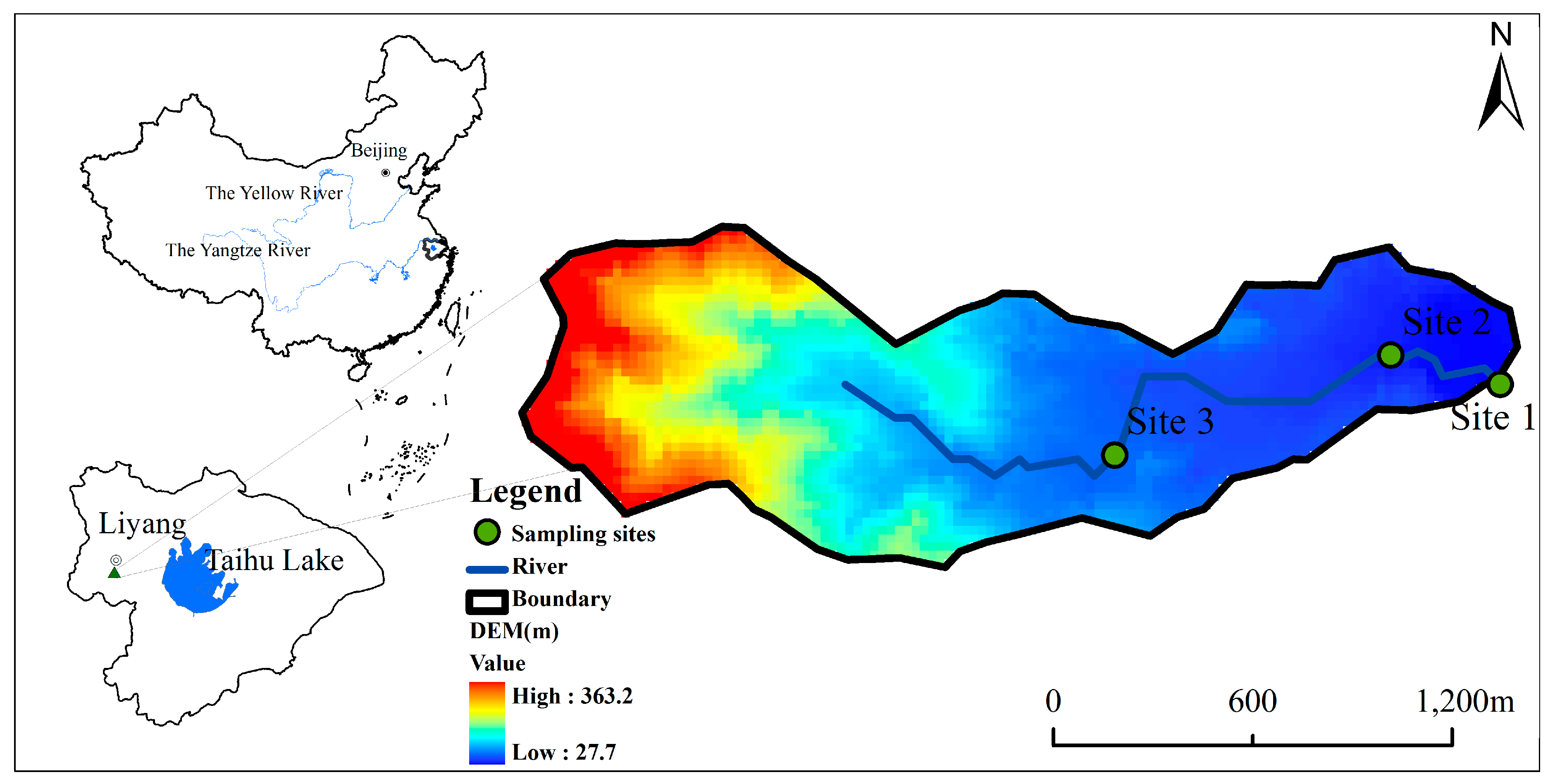
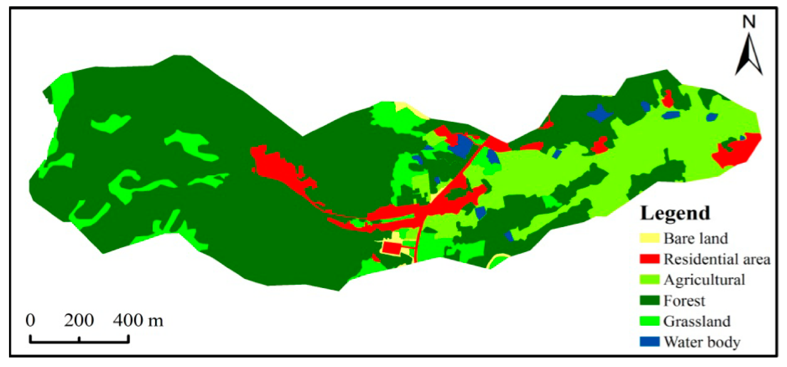
In this study, AnnAGNPS version 5.1 was applied. AnnAGNPS is a batch-process, continuous simulation, watershed-scale model designed to aid in the evaluation of long term, hydrologic and water quality responses to agricultural management practices [27]. It was jointly developed by the United States Department of Agriculture (USDA), the Agricultural Research Service (ARS) and the Natural Resources Conservation Service (NRCS) [28]. It consists of a system of computer models developed to predict NPS pollutant loadings within an agricultural watershed [16]. With the support of a routing system, continuous simulation has been realized [29]. The model simulates runoff, sediments, nutrients and pesticides, leaving the land surface and shallow subsurface and moving through the channel system to the watershed outlet, with output available atthe event, monthly and annual scales [30]. AnnAGNPS model is also designed to assist in determining BMPs (Best Management Practices), TMDLs (Total Maximum Daily Loads), and in risk cost/benefit analysis.

In AnnAGNPS, the analyzed watershed can be divided into many homogenous (in terms of soil type, land use and land management) cells or subwatersheds (up to 40 km²) to quantitatively estimate precipitation runoff and sediment, as well as nutrient and pesticide loadings [16,31]. The cells are irregular basins with comparatively uniform physical and hydrological characteristics, which allows for the analysis of any point within the watershed. The physical or chemical constituents are routed from each cell and are either deposited within the reaches or transported out of the watershed [4]. Cells and reaches and their topographic properties can be estimated by TOPAGNPS (Topographic Parameterization program used for AGNPS) and AGFLOW (Agricultural watershed Flownet generation program), which are additional modeling components in AnnAGNPS [32].

Surface runoff is estimated based on the Soil Conservation Service [33] Curve Number (CN) method. CN represents the runoff producing potential of soils, and has a range of 0–100. The Revised Universal Soil Loss Equation (RUSLE) [34] is used to estimate the daily sheet and rill erosion of the area. Considering that the RUSLE does not simulate the transport of eroded particles, the Hydro-Geomorphic Universal Soil Loss Equation (HUSLE) is used to simulate sediment delivery to the stream [35]. For N and P, a basic mass conservation equilibrium is employed to estimate nutrients generation and loading for rainfall events [36]. The model has a fixed N and P cycle, which considers the amounts of N and P joining or leaving the watershed [15].

2.2. Study Area

The study watershed is named Wucun and is located in the western basin of Taihu Lake in China. The area of the watershed is 1.81 km² (181ha). The river originates from low hilly terrain with a maximum elevation of approximately 360 m, and it travels 2500 m while finding its way to the outlet (sampling stations), which is at an elevation of approximately 27 m (Site 1) (Figure 1). The watershed is characterized by a subtropical monsoon climate, with a mean annual rainfall of 1169.3 mm and an annual average temperature of 15.4 °C (2005–2013), and the rainy seasons mainly occur over 4–9 months. The soil type in the upstream of the watershed is generally Typic Ali-Udic Argosols (TAUA) and that in the downstream of the watershed is Typic Hapli-Stagnic Anthrosols (THSA). Properties of soils are presented in Table 1. The land use in this watershed is largely dominated by forest, and other land uses mainly include urban land and agriculture.

Figure 1. The Map of the Wucun watershed showing sampling sites, the digitized stream and the watershed boundary.

Figure 1. The Map of the Wucun watershed showing sampling sites, the digitized stream and the watershed boundary.

Table 1. Properties of soils in the study area.

Classification [37]	Hydrological	K Factor Value	Depth (mm)	Content (%)
				Clay	Silt	Sand	Very Fine Sand
TAUA	B	0.04	0–16	15.12	41.98	42.9	3.01
			16–29	17.41	37.69	44.9	3.11
			29–56	16.84	40.26	42.9	3.01
THSA	C	0.04	0–14	19.22	53.06	27.72	1.97
			14–24	12.9	59.38	27.72	1.97
			24–36	12.73	57.3	29.97	2.12
			36–100	13.26	31.21	55.53	3.50

Table 1. Properties of soils in the study area.

Classification [37]	Hydrological	K Factor Value	Depth (mm)	Content (%)
				Clay	Silt	Sand	Very Fine Sand
TAUA	B	0.04	0–16	15.12	41.98	42.9	3.01
			16–29	17.41	37.69	44.9	3.11
			29–56	16.84	40.26	42.9	3.01
THSA	C	0.04	0–14	19.22	53.06	27.72	1.97
			14–24	12.9	59.38	27.72	1.97
			24–36	12.73	57.3	29.97	2.12
			36–100	13.26	31.21	55.53	3.50

2.3. Data Acquisition

2.3.1. Climate Data

Climate data required for running the AnnAGNPS model includes maximum temperature, minimum temperature, precipitation, dew point temperature, sky cover or solar radiation, and wind speed. In this study, the time span of climate data was nine years from January 2005 to December 2013. Data of maximum temperature, minimum temperature, and precipitation were downloaded from the Liyang national climate station (31°26′N, 119°29′E; at 7.7m height) for 2005 to 2010 and were provided by the Nanjing Institute of Geography and Limnology, Chinese Academy of Sciences from 2011 to 2013. Additionally, dew point temperature was calculated from the relative humidity and mean air temperature, and solar radiation was deduced from temperature and sunshine duration, as suggested by the China Meteorological Administration (CMA) [38].

2.3.2. Topographic Data

This study utilized a 1:50,000 relief map, which was scanned and then digitized to construct a Digital Elevation Model (DEM) (30 m ×30 m). The DEM is used for topographic evaluation, drainage identification, watershed segmentation, and subcatchment parameterization.CSA (Critical Source Area) and MSCL (Minimum Source Channel Length) are employed to divide the watershed. The CSA value defines a minimum drainage area below which a permanent channel is defined, and the MSCL is the minimum acceptable length of the cell swale for the source channel to exist. Various combinations of CSA/MSCL values were tried for watershed delineation. Finally, values of 2 ha and 70 m were adopted to define CSA and MSCL, respectively. As a result, 78 cells and 36 reaches were obtained, and the cell area ranged from 428 to 157,940 m².

2.3.3. Soil Data

Running the AnnAGNPS model requires specific properties of all soil layers. The physical properties include particle size distribution, bulk density, saturated hydraulic conductivity, field capacity, wilting point, etc. Chemical properties such as pH, organic matter, organic and mineral nitrogen and phosphorous were considered. The digital soil map obtained from the Soil Survey Office in Jiangsu Province of China provided little information about the properties of soil. Thus, parts of properties such as saturated hydraulic conductivity, field capacity and wilting point were calculated by the Soil Water Characteristics (SWCT) module of the SPAW (Soil Plant Atmosphere Water) model [39]. Additionally, the soil erodibility factor (K) was derived following Wischmeier and Smith [40]. The soil properties for various types of soil in the study area are shown in Table 1.

2.3.4. Land Use Data

The original land use map was obtained from an aerial image taken in 2009 with a resolution of 0.5 m × 0.5 m. The image data of the study watershed was reclassified into six types of land uses by visual interpretation. As shown in Figure 2, most of the study area was covered by forest and agricultural land use types with proportions of 66% and 17%, respectively. The remaining area was covered by the bare land, urban land, grass land and water body land-use types. The agriculture is rotated between rice and rape. The information concerning the management schedule (Table 2) was obtained by interviewing local farmers.

Figure 2. Land use map of the Wucun watershed.

Figure 2. Land use map of the Wucun watershed.

Table 2. Schedules of annual cultivation and agricultural practices in the Wucun watershed.

Land Use	Date	Operation	Observation
Rice	21 May	Seeding	Combined seeding machine
	12 June	Fertilization	Carbamide
	10 July	Fertilization	Ammonium bicarbonate
	10 August	Fertilization	Compound fertilizer
	25 August	Weeding	Triadimefon/Diniconazole
	3 September	Fertilization	Compound fertilizer
	18 October	Grain harvesting	5000–6000kg·ha−1
	25 October	Tillage	Moldboard
Rape	1 November	Seeding	Combined seeding machine
	10 December	Fertilization	Carbamide
	5 February	Fertilization	Carbamide
	10 March	Fertilization	Carbamide
	11 March	Fertilization	Ammonium bicarbonate
	10 May	Grain harvesting	2200–3000kg·ha−1
	18 May	Tillage	Moldboard

Table 2. Schedules of annual cultivation and agricultural practices in the Wucun watershed.

Land Use	Date	Operation	Observation
Rice	21 May	Seeding	Combined seeding machine
	12 June	Fertilization	Carbamide
	10 July	Fertilization	Ammonium bicarbonate
	10 August	Fertilization	Compound fertilizer
	25 August	Weeding	Triadimefon/Diniconazole
	3 September	Fertilization	Compound fertilizer
	18 October	Grain harvesting	5000–6000kg·ha−1
	25 October	Tillage	Moldboard
Rape	1 November	Seeding	Combined seeding machine
	10 December	Fertilization	Carbamide
	5 February	Fertilization	Carbamide
	10 March	Fertilization	Carbamide
	11 March	Fertilization	Ammonium bicarbonate
	10 May	Grain harvesting	2200–3000kg·ha−1
	18 May	Tillage	Moldboard

2.3.5. Hydrologic and Nutrient Loading Data

Due to the lack of long-term runoff records in the Wucun watershed, the realistic annual runoff was estimated by an empirical formula of rainfall–runoff [41], which was developed in the similar hilly region of the Taihu Lake watershed. Thus, the simulated annual runoff at Site 1 (Figure 1) could be compared with the estimated one to calibrate and validate the AnnAGNPS model. Regarding the climate data, data from 2005–2009 were used for annual calibration, and data from 2010 to 2013 were used for annual validation.

Monthly water samples (total nitrogen and total phosphorus) at three monitoring sites (see Figure 1) were sampled and then analyzed in the laboratory during December 2012 to December 2013. Monthly runoff data were also measured at this period. Thus, the nutrient loadings were calculated by multiplying nutrient concentrations by monthly runoff. The monthly runoff could be calibrated at Site 1, while Site 2 and Site 3 were employed to validate the simulation processes. For nutrients, there was a similar process to that of monthly runoff. Site 1 was chosen to calibrate the nutrients, and Site 2 and Site 3 were used for validation. This calibration and validation method is similar to a random spot check, which may more accurately reflect the efficiency of the model.

2.4. Parameter Sensitivity Analysis

Sensitivity analysis is a methodological study of the response to the selected output variables to variations in parameters and driving variables [5]. It has been widely applied in hydrological models such as SWAT [42,43] and HSPF [44] to help users identify crucial parameters.

2.4.1. Runoff Parameter

Most of the worldwide studies evaluating AnnAGNPS [19,22,30,45] showed that CN is the most sensitive parameter to surface runoff prediction, and these studies were successfully calibrated for surface runoff simulation by adjusting CN values. Therefore, in this study, we also make the simulated runoff approximate the actual runoff by adjusting the values of CN.

2.4.2. Nutrients parameters

The nutrient parameters used in some literature [4,15,31,46] are not clear. These studies predicted nutrients by using the AnnAGNPS model, but the correlative parameters that they used were not reported. Additionally, some previous studies had made some contributions to analyzing the sensitivity parameters for nutrients [5,47,48]. Yuan et al. [47,48] indicated that the Initial nitrogen concentration in the soil, Plant uptake and Fertilizer mixing code were sensitive parameters for nitrogen loading, and Initial soil p contents as well as p application rate were sensitive parameters for phosphorus loading. Liu [5] concluded that CN, Rainfall quantity, Fertilizer application and Fertilizer available were sensitive parameters for both total nitrogen (TN) and total phosphorus (TP).

In this study, sensitivity analysis was considered necessary, and was carried out before calibration for nutrients. Parts of the parameter values were obtained from the survey data, such as Initial soil N and p contents, as mentioned above. We mainly wanted to evaluate the effects of human factors on nutrient simulation, including the fertilizer and crop parameters Residue Mass Ratio, Root Mass, Canopy Cover, Fertilizer Rate, Fertilizer Depth, Fertilizer Inorganic, and Fertilizer Organic. Based on a literature review [16,49,50], Differential Sensitivity Analysis (DSA) was employed to evaluate the sensitivity due to its simplicity and low-need for computation time. The DSA calculate one point in the parameter space by adjusting the parameter with a fixed percentage while the other factors remain constant. As shown below, each selected parameter would be changed by an increment of ∆x = ±10%, ±20%, ±30%, ±40%, ±50%, ±60% while fixing the values of the other parameters. The gradient of the output response with respect to the selected parameter was used to quantify the degree of sensitivity I. Each term of ∆x would have a value of I′, and I was defined by the average of the six terms. I′ was computed as follows:

$$I\prime =\frac{\left(y_2-y_1\right)/y_0}{2△x/x_0}$$

(1)

The model output y₀ is calculated with an initial value x₀ of the parameter x; x₀ is varied by ±∆x, yielding x₁= x₀−Δx and x₂ = x₀+ Δx; and y₁ and y₂ correspond to x₁ and x₂.

The Sensitivity Index is ranked into four categories [51] as follows: less than 0.05—small to negligible sensitivity; 0.05–0.2—medium sensitivity; 0.2–1.0—high sensitivity; and more than 1.0—very high sensitivity.

2.5. Evaluation of Model Performance

The results of the simulation were analyzed for “goodness-of-fit” with the observed data. The performance evaluation of AnnAGNPS was carried out in a comprehensive manner, as suggested by Legates and McCabe et al. [20,52,53]. The coefficient of determination (R²), coefficient of efficiency (E), root mean square error (RMSE), and coefficient of residual mass (CRM) were employed for model assessment. Additionally, it should be noted that R² and E are overly sensitive to extreme values, which may mislead the evaluation of model performance. To avoid this, a revised coefficient of efficiency was defined as E′, which could reduce the effect of squared terms [52].The formulas for these coefficients are listed in following.

The coefficient of determination ranges from 0 to 1, with higher values indicating better agreement and is given as:

$$R^2={\left\{\frac{{\displaystyle \sum _{i=1}^N\left(O_i-\overline{O}\right)\left(S_i-\overline{S}\right)}}{\sqrt{{\displaystyle \sum _{i=1}^N{\left(O_i-\overline{O}\right)}^2}}\sqrt{{\displaystyle \sum _{i=1}^N{\left(S_i-\overline{S}\right)}^2}}}\right\}}^2$$

(2)

The coefficient of efficiency E is given as:

$$E=1-\frac{{\displaystyle \sum _{i=1}^N{\left(O_i-S_i\right)}^2}}{{\displaystyle \sum _{i=1}^N{\left(O_i-\overline{O}\right)}^2}}$$

(3)

E is dimensionless and ranges from minus infinity to 1. As proposed by Van [54], the results are highly satisfactory for an E value equal or larger than 0.75, satisfactory between 0.36 and 0.75, and unsatisfactory for an E value smaller than 0.36.

The modified coefficient of efficiency is calculated as:

$$E\prime =1-\frac{{\displaystyle \sum _{i=1}^N\left|O_i-S_i\right|}}{{\displaystyle \sum _{i=1}^N\left|O_i-\overline{O}\right|}}$$

(4)

In general, $E\prime$ has a lower value than E, and the model can be considered satisfactory when $E\prime$ ranges from 0.51 to 0.71 [20].

The root mean square error (RMSE) is given as:

$$RMSE=\sqrt{{\frac{{\displaystyle \sum _{i=1}^N\left(O_i-S_i\right)}}{N}}^2}$$

(5)

The coefficient of residual mass (CRM) is given as:

$$CRM=\frac{{\displaystyle \sum _{i=1}^N{O}_i-{\displaystyle \sum _{i=1}^N{S}_i}}}{{\displaystyle \sum _{i=1}^N{O}_i}}$$

(6)

where O_i is the observed data, S_i is the simulated data, $\overline{O}$ is the mean of the observed data set, $\overline{S}$ is the mean of the simulated data set, i is the ith event, and N is the number of observations.

3. Results and Discussion

During the nine-year study period, annual rainfalls ranged from 828.10 to 1267.50 mm with a mean and standard deviation of 1052.92 and 122.60 mm, respectively. At the monthly scale, only the runoff data from 2013 were available, and the recorded rainfalls were in the range of 10–136.60 mm with resulting runoff varying from 4.43 mm to 53.23 mm. Approximately 45% of rainfall was concentrated from May to July.

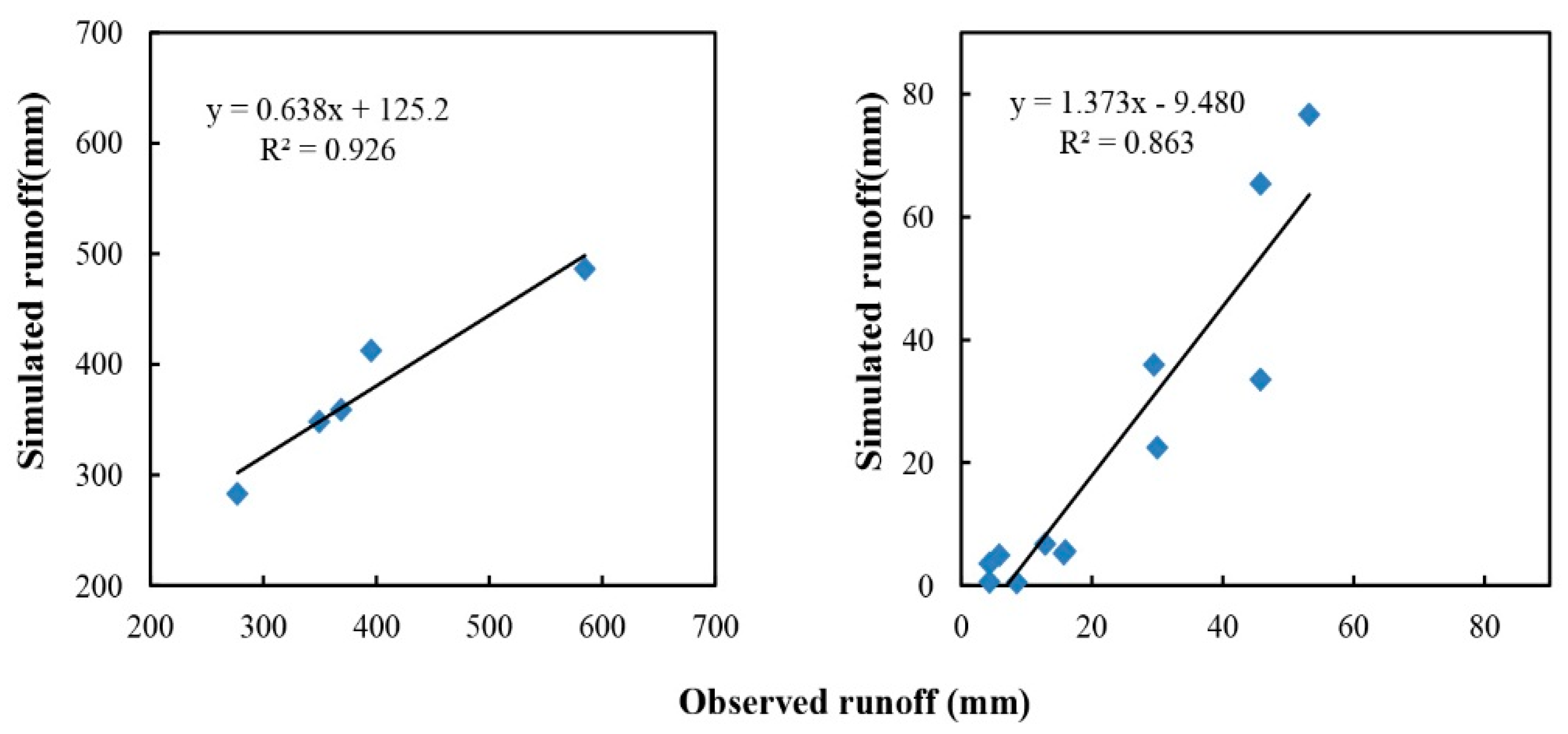
3.1. Runoff Calibration

In watershed modeling, calibration and validation are important steps for ensuring the quality of model simulations. Upon completion of the data entry using the AnnAGNPS Data Input Editor, runoff was calibrated by adjusting CN for all landuse categories. The best results (Figure 3) were obtained by increasing the CN values of agriculture, forest, grassland and urban land by 20%, 30%, 20%, 20%, respectively (Table 3). Before calibration, E and E′ both had negative values, and the CRMs had high values (Table 4). These parameters indicated that substantial differences existed between simulations and observations. However, acceptable statistical parameters were obtained after calibration processes. As shown in Table 4, at annual scale, the difference between simulated and observed average annual runoff was very small (as indicated by small CRMs), and the other statistical parameters included R² = 0.93, E = 0.81, and E′ = 0.65. At the monthly scale, the statistical analyses showed that R² = 0.86, E = 0.59, E′ = 0.39 and CRM = 0.04.

Monthly scale simulation was barely satisfactory. Some months were overestimated, whereas some were underestimated. The main reason for this is that the monthly runoff data were calculated from the measured data when sampling in the middle of each month. This process may lead to a large difference for the actual flow, especially in the rainy or dry periods, and it may yield a smaller or larger result when estimating the monthly runoff based on this value.

Figure 3. Comparison between observed and simulated runoff at annual (left) and monthly (right) scales for calibration process.

Figure 3. Comparison between observed and simulated runoff at annual (left) and monthly (right) scales for calibration process.

Table 3. Initial and final CN values for each land-use type.

Land Use	Curve Numbers for Hydrologic Soil Groups
	Initial Values				Final Values
	A	B	C	D	A	B	C	D
Bare land	65	75	82	95	65	75	82	95
Residential area	55	68	79	85	66	82	95	99
Agricultural	60	72	80	85	78	86	96	99
Forest	48	60	73	80	58	78	95	96
Grass land	42	69	79	87	50	83	95	98

Table 3. Initial and final CN values for each land-use type.

Land Use	Curve Numbers for Hydrologic Soil Groups
	Initial Values				Final Values
	A	B	C	D	A	B	C	D
Bare land	65	75	82	95	65	75	82	95
Residential area	55	68	79	85	66	82	95	99
Agricultural	60	72	80	85	78	86	96	99
Forest	48	60	73	80	58	78	95	96
Grass land	42	69	79	87	50	83	95	98

Table 4. Estimated statistical parameters of model performance for default and calibration/validation.

Items	Calibration					Validation
	R2	E	E′	RMSE	CRM	R2	E	E′	RMSE	CRM
Annual scale
Run off	0.93(0.76) *	0.81(−5.32)	0.65(−2.23)	45.09(257.83)	0.05(0.63)	0.88(0.82)	0.86(−8.00)	0.65(−2.2)	26.95(213.62)	−0.02(0.58)
Monthly scale
Run off	0.86(0.55)	0.59(−3.21)	0.39(−1.33)	11.24(21.58)	0.04(0.62)	0.84(0.75)	0.65(−2.64)	0.42(−1.75)	10.65(20.31)	0.02(0.59)
						0.87(0.78)	0.81(−1.63)	0.62(−0.55)	8.71(15.16)	0(0.45)
TN	0.91(0.77)	0.86(0.33)	0.71(0.12)	100(180.25)	0.22(0.87)	0.92(0.85)	0.71(0.29)	0.58(0.08)	130.85(210.34)	0.42(0.92)
TP	0.66(0.38)	0.37(−1.05)	0.46(0.10)	1.67(3.15)	0.14(0.92)	0.62(0.28)	0.18(−1.26)	0.37(−0.55)	1.18(2.67)	0.19(0.88)

* Numbers in parenthesis are default values.

Table 4. Estimated statistical parameters of model performance for default and calibration/validation.

Items	Calibration					Validation
	R2	E	E′	RMSE	CRM	R2	E	E′	RMSE	CRM
Annual scale
Run off	0.93(0.76) *	0.81(−5.32)	0.65(−2.23)	45.09(257.83)	0.05(0.63)	0.88(0.82)	0.86(−8.00)	0.65(−2.2)	26.95(213.62)	−0.02(0.58)
Monthly scale
Run off	0.86(0.55)	0.59(−3.21)	0.39(−1.33)	11.24(21.58)	0.04(0.62)	0.84(0.75)	0.65(−2.64)	0.42(−1.75)	10.65(20.31)	0.02(0.59)
						0.87(0.78)	0.81(−1.63)	0.62(−0.55)	8.71(15.16)	0(0.45)
TN	0.91(0.77)	0.86(0.33)	0.71(0.12)	100(180.25)	0.22(0.87)	0.92(0.85)	0.71(0.29)	0.58(0.08)	130.85(210.34)	0.42(0.92)
TP	0.66(0.38)	0.37(−1.05)	0.46(0.10)	1.67(3.15)	0.14(0.92)	0.62(0.28)	0.18(−1.26)	0.37(−0.55)	1.18(2.67)	0.19(0.88)

* Numbers in parenthesis are default values.

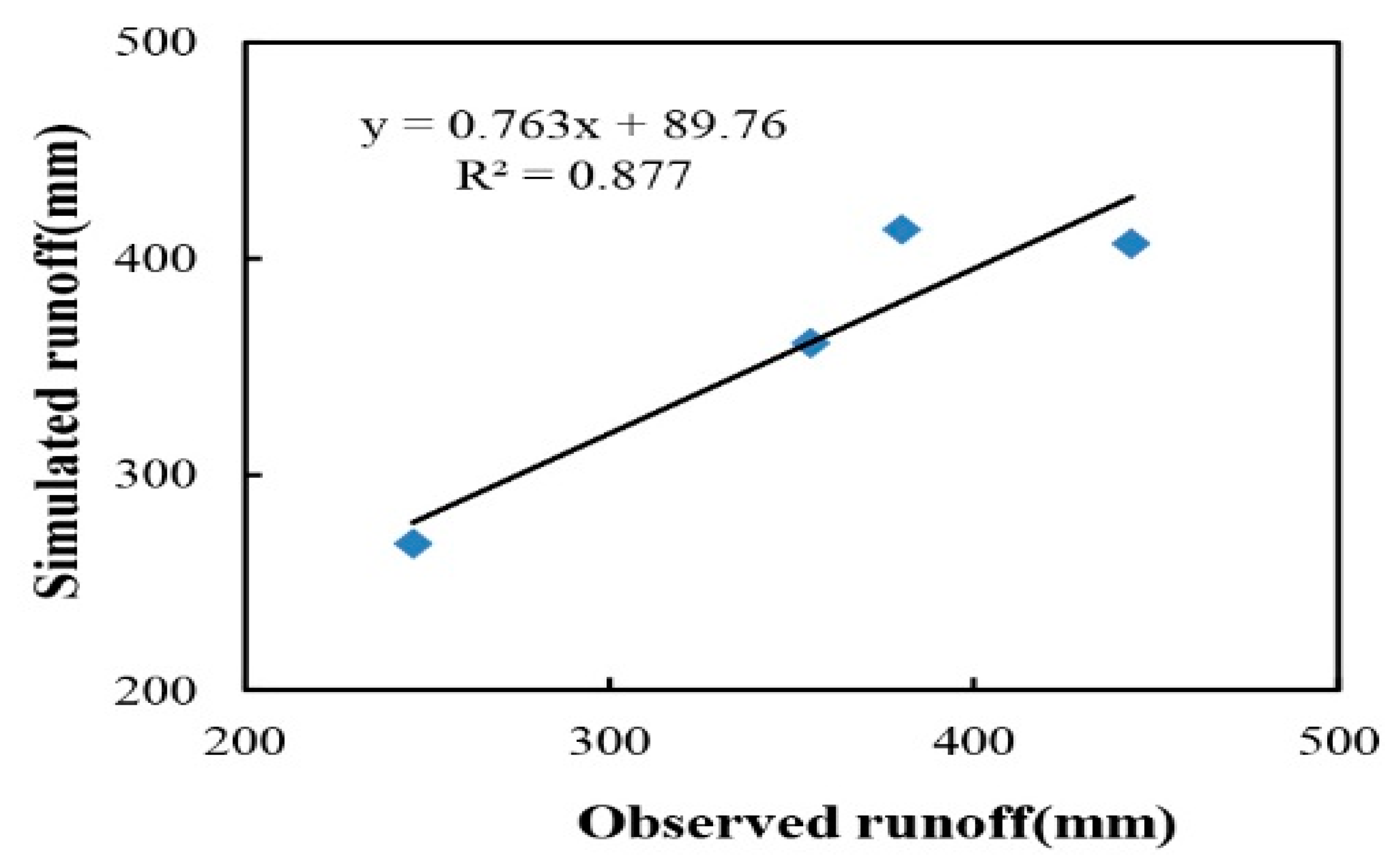
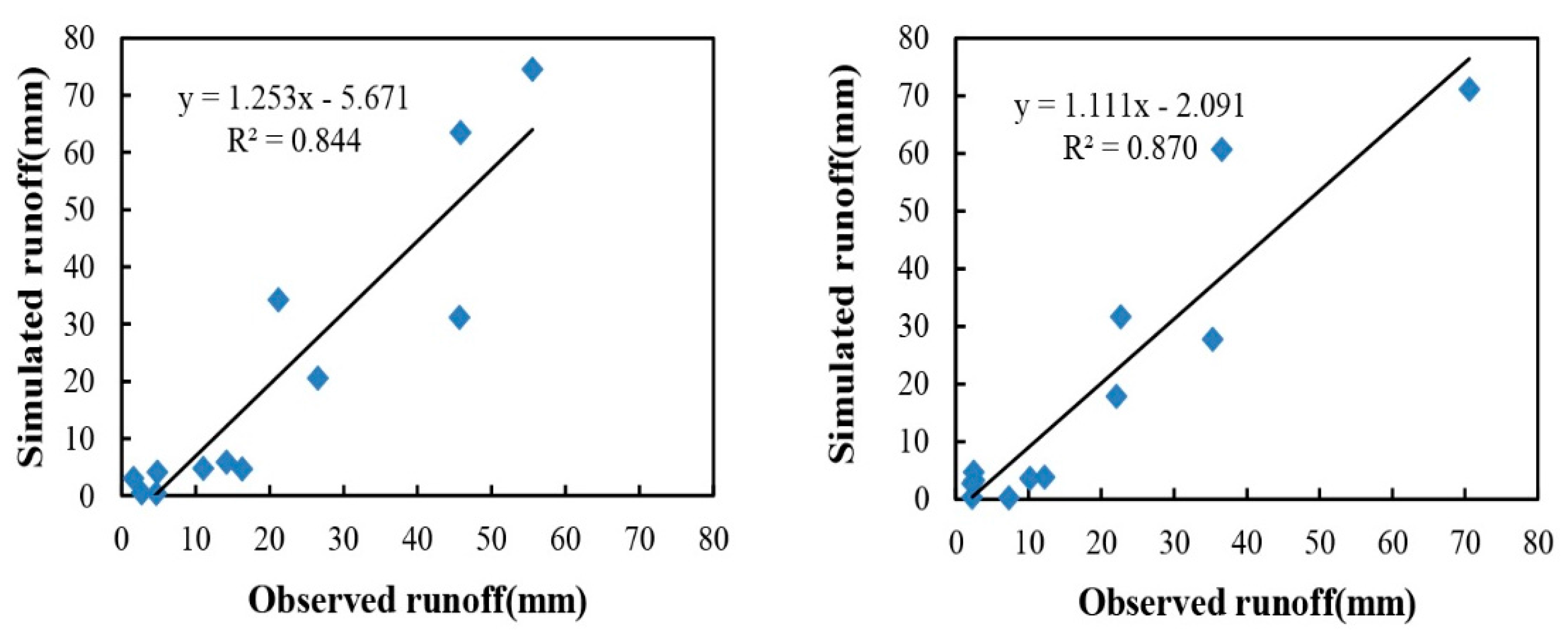
3.2. Runoff Validation

Validation was carried out after calibration. At the annual scale (Figure 4), the difference between simulated and observed runoff was only approximately 2.6%, with averages of 361.98 mm and 356.34 mm, respectively, and with E = 0.86, E′ = 0.65, and CRM = −0.02. At the monthly scale (Figure 5), two sites were employed to validate the simulation process, with values of 0.65 and 0.81 for E, and 0.42 and 0.62 for E′ at Site 2 and Site 3, respectively. Both of these results confirm the ability of the model to predict runoff after calibration.

Figure 4. Comparison between observed and simulated runoff at the annual scale for the validation process.

Figure 4. Comparison between observed and simulated runoff at the annual scale for the validation process.

Figure 5. Comparison between observed and simulated monthly runoff at Site 2 (left) and Site 3 (right) during validation process.

Figure 5. Comparison between observed and simulated monthly runoff at Site 2 (left) and Site 3 (right) during validation process.

Site 3 performed more efficient than Site 2 during the validation process. In the geography, Site 3 is upstream of Site 2, and thus the watershed based on Site 3 as the outlet is smaller than that based on Site 2. As noted by Chahor and Taguas [16,17], the smaller the watershed is, the more satisfactory the model prediction seems to be. Additionally, the cultivated areas mainly concentrate between Site 2 and Site 3, and agricultural irrigation is also a factor affecting the validation accuracy of Site 2. Nevertheless, Site 2 is still in the range of required accuracy for the model evaluation. In the validation process, both of the two sites yield satisfactory results, thus confirming the accuracy of the calibration process.

3.3. Nutrient

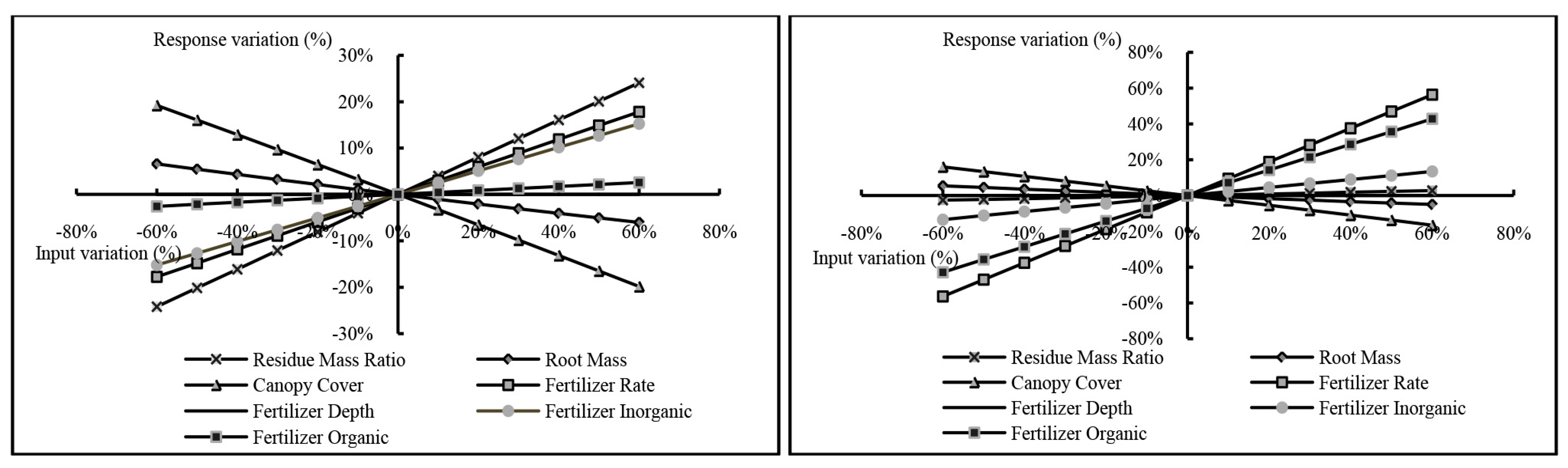
3.3.1. Results of the Parameter Sensitivity Analysis

Figure 6 depicts the relationship between input variation and output variation, where most of the selected parameters had a linear effect on nutrient loading prediction. Fertilizer rate, Fertilizer organic, Fertilizer inorganic, and Residue mass ratio had positive correlations (Pearson Correlation = 1, p < 0.01) with the nutrient loading model output, while the Root mass and Canopy cover had negative correlations (Pearson Correlation = −1, p < 0.01). This might be explained by more fertilizer leading to more nutrient loss; otherwise, more vegetation could reduce nutrient loss.

Figure 6. The sensitivity of nutrient for (left) TN and (right) TP to the selected input parameters

Figure 6. The sensitivity of nutrient for (left) TN and (right) TP to the selected input parameters

According to Lenhart [51], Fertilizer rate, Fertilizer organic, Canopy cover and Fertilizer inorganic can be classified as high sensitive parameters for TN output, whereas Residue mass ratio, Fertilizer rate, Fertilizer inorganic, and Canopy cover are highly sensitive parameters for TP output. The remaining parameters have small to negligible sensitivity and medium sensitivity (Table 5).

Table 5. Sensitivity classification of AnnAGNPS input parameters to nutrient loading.

Input Parameters	Sensitivity Index for TN	Sensitivity Index for TP
Residue mass ratio	0.04	0.39
Root mass	−0.09	−0.10
Canopy cover	−0.26	−0.32
Fertilizer rate	0.94	0.30
Fertilizer depth	0.00	0.00
Fertilizer inorganic	0.25	0.26
Fertilizer organic	0.69	0.04

Table 5. Sensitivity classification of AnnAGNPS input parameters to nutrient loading.

Input Parameters	Sensitivity Index for TN	Sensitivity Index for TP
Residue mass ratio	0.04	0.39
Root mass	−0.09	−0.10
Canopy cover	−0.26	−0.32
Fertilizer rate	0.94	0.30
Fertilizer depth	0.00	0.00
Fertilizer inorganic	0.25	0.26
Fertilizer organic	0.69	0.04

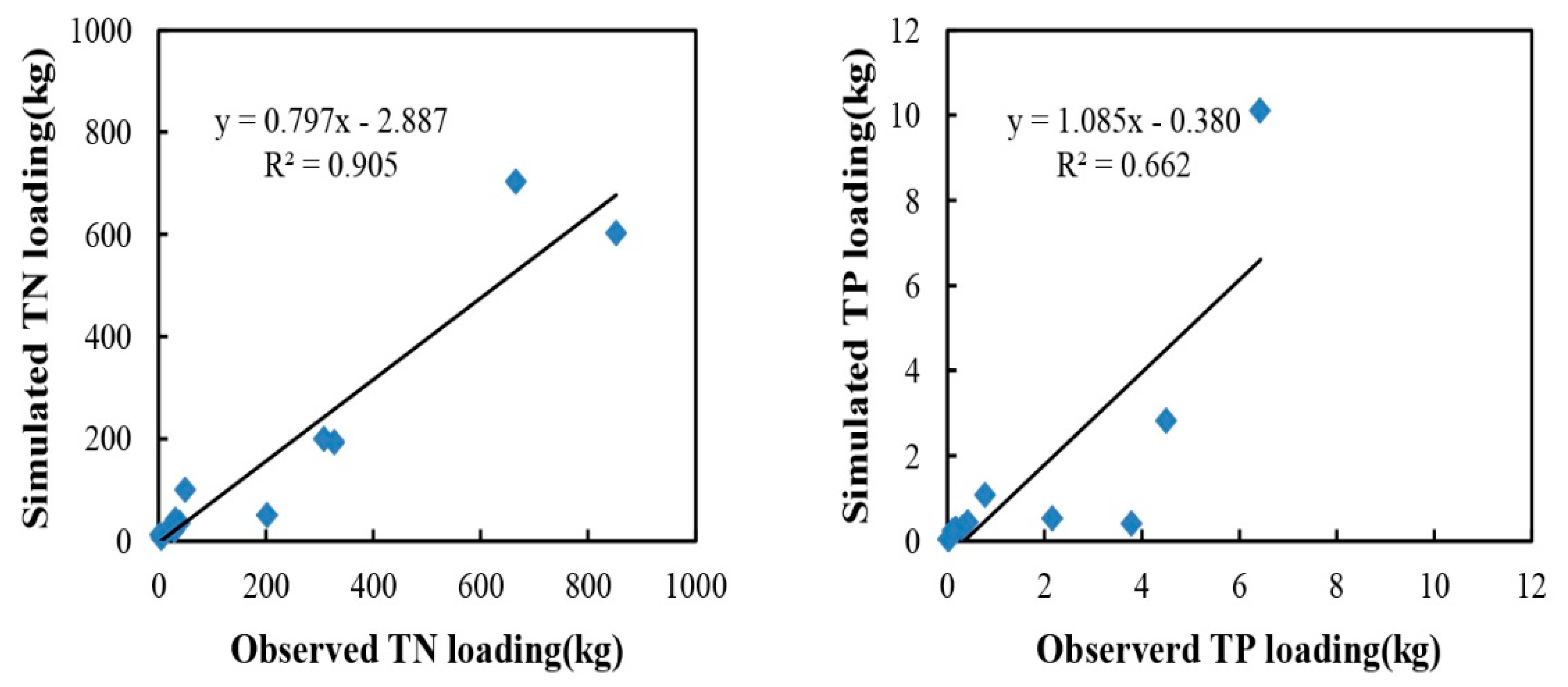
3.3.2. Nutrient Calibration

Similar to runoff calibration, nutrient calibration was also made for Site 1. Due to the lack of nutrient data, only monthly TN and TP loadings were investigated in this study. Based on the result of parameters sensitivity analysis, calibration was first carried out by adjusting the most sensitive parameters, and then adjusting the medium-sensitivity parameters. Several efforts were made before obtaining the final result. Figure 7 (left) shows the plot of simulated versus observed TN loadings with regression. The value of CRM was 0.22 > 0, indicating under-prediction and yielding an R² value of 0.91. The coefficient of efficiency and modified coefficient of efficiency for TN loadings showed satisfactory results of 0.86 and 0.71 (Table 4), respectively. Moreover, TP loading was also slightly under-predicted (CRM = 0.14). As shown in Figure 7 (right), the coefficient of determination (R²) was found to be 0.66, which meant that the model was only able to explain or represent approximately 66% of the varieties in the observed data. The results for E and E′ were 0.38 and 0.46, respectively.

Figure 7. Comparison between observed and simulated TN (left) and TP (right) loading during the calibration process.

Figure 7. Comparison between observed and simulated TN (left) and TP (right) loading during the calibration process.

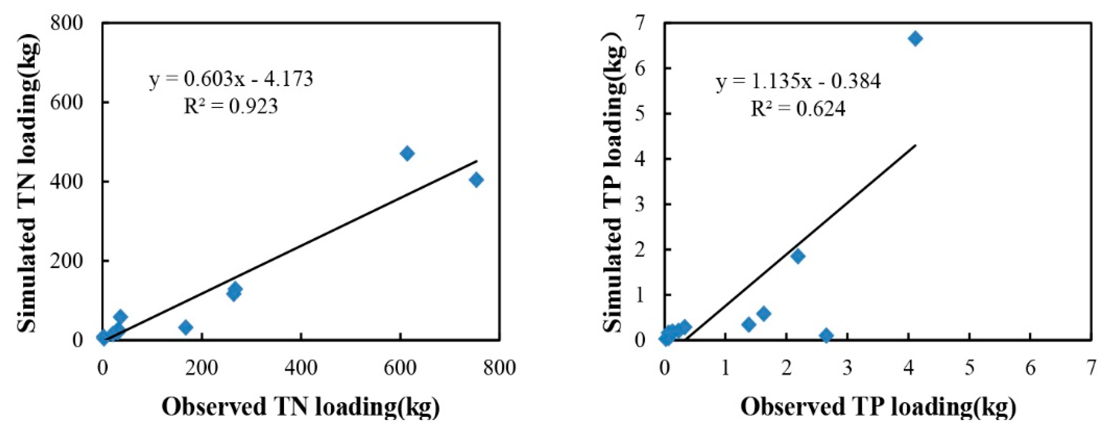
3.3.3. Nutrient Validation

The validation process was performed for Site 2 and Site 3 (Figure 1). Figure 8 shows the plot of simulated versus observed loading for TN and TP in Site 2. TN prediction performed well, with an R² value of 0.92 (Figure 8, left) and a CRM value of 0.42. The coefficient of efficiency and modified coefficient of efficiency for TN loading also showed satisfactory results of 0.71 and 0.58, respectively. These statistical values suggested that the model was able to correctly predict the site conditions. For the TP, R² was 0.624 (Figure 8, right), the results for E and E′ were slightly poor at 0.18 and 0.37, respectively, but the CRM of 0.19 was acceptable (Table 4). The largest difference occurred in October, where the observed and simulated TP loading were 2.66 kg and 0.09 kg, respectively.Clearly, they made a substantial contribution to the low performance of TP. Although the TP prediction was not satisfactory, it was still able to represent a certain portion of the observed data.

The model performed satisfactorily for TN simulation at Site 2. Otherwise, TP simulation was poor at this site. Under-predicted values for TP clearly existed in the calibration and validation processes (Figure 7 and Figure 8). A lack of reliable information may have leaded to this underestimation, as information such as plant uptake and other natural phosphorus cycling were taken from unofficial sources.Many vital input parameters are needed for calibration purposes. The performance at Site 3 was poor, as large differences were observed in both TN and TP validation processes. The mean values of simulated and observed TN loading were 0.56 kg and 143.5 kg, and those of TP were 0.007 kg and 0.96 kg, respectively. The reason may be that Site 3 was located in the urban area, its concentrations of TN and TP were deeply affected by the residential activities, and the samplings from this site would yield high values. Thus, this site was not suitable for the calibration or validation processes.

Figure 8. Comparison between observed and simulated TN (left) and TP (right) loading during the validation process.

Figure 8. Comparison between observed and simulated TN (left) and TP (right) loading during the validation process.

Compared with previous studies applying the AnnAGNPS model to simulate nutrients, this study obtained similar or better results. Shamshad [15] reported the application of the AnnAGNPS model to a watershed (63.09 km²) with conditions and climate typical of Malaysia. In their evaluation of the model performance, the model performed satisfactorily for runoff simulation. However, poor statistical parameters were obtained for TN and TP simulation processes. The results of Pease’s simulation [4] also showed low performance for nutrient simulation in an east-central North Dakota watershed with an area of 1697 km². Baginska [25] evaluated the model in a 2.55 km² watershed of Currency Creek, Australia, and concluded that the model produced satisfactory results for event flows, but it yielded a high degree of uncertainty for nitrogen. Thus, it can be seen that the model had experienced low nutrient simulation performance at various scales. Additionally, the low performance of AnnAGNPS in predicting nutrient loading is also reported in other studies [31,55,56]. Due to the mechanism of the AnnAGNPS model where nutrient loading is based on mass conservation, any missing input or output information of nutrients in watershed will considerably affect the results. Furthermore, Bingner [36] noted that the model assumed that there was no tracking of nutrients from one day to the next, which means that there will definitely be a loss of mass. Additionally, a lack of reliable information and data regarding nutrients is a common phenomenon in many areas, and this may further contribute to the low performance of nutrient prediction. More detailed data should be monitored to obtain a more realistic watershed simulation.

4. Conclusions

The AnnAGNPS model was applied in a small agricultural watershed called “Wucun” in the upstream of the Taihu watershed to validate its capability to predict surface runoff and to test its capability to predict nutrient loading using data recorded from January 2005 to December 2013.

The model was calibrated in the period of 2005–2009 to achieve the best-fit runoff prediction, as runoff has a major impact on nutrient prediction. This was completed by adjusting the CN values. Then, the model was validated in the period of 2010–2013. The result was evaluated for “goodness-of-fit” between predicted and observed data using five statistical measures, namely the root mean square error (RMSE), coefficient of residual mass (CRM), coefficient of determination (R²), coefficient of efficiency (E) and modified coefficient of efficiency (E′). The values of the five parameters indicated a good correlation between the predicted and observed data, which suggested that the model possessed an adequate capability to simulate surface runoff.

Concerning nutrient loading, a parameter sensitivity analysis was first carried out to evaluate the sensitivity of the nutrient parameters. Fertilizer rate, Fertilizer organic, Canopy cover and Fertilizer inorganic were more sensitive to TN output, and Residue mass ratio, Fertilizer rate, Fertilizer inorganic and Canopy cover were more sensitive to TP output. The AnnAGNPS model was then calibrated based on the sensitivity analysis results. TN simulation produced satisfactory results for both the calibration and validation processes, whereas TP loading performance was slightly poor. Though the results were not very good, the model was still able to represent a certain portion of variability in the observed data. Generally, the study found that the AnnAGNPS model was qualified as a watershed modeling tool.

References

1. Arnold, J.G.; Allen, P.M.; Bernhardt, G. A comprehensive surface-groundwater flow model. J. Hydrol. 1993, 142, 47–69. [Google Scholar] [CrossRef]
2. Walton, R.S.; Hunter, H.M. Isolating the water quality responses of multiple land uses from stream monitoring data through model calibration. J. Hydrol. 2009, 378, 29–45. [Google Scholar] [CrossRef]
3. Diaz-Ramirez, J.; Martin, J.L.; William, H.M. Modelling phosphorus export from humid subtropical agricultural fields: A case study using the HSPF model in the Mississippi Alluvial Plain. J. Earth Sci. Clim. Chang. 2013, 4. [Google Scholar] [CrossRef]
4. Pease, L.M.; Oduor, P.; Padmanabhan, G. Estimating sediment, nitrogen, and phosphorous loads from the pipestem creek watershed, North Dakota, using AnnAGNPS. Comput. Geosci.UK 2010, 36, 282–291. [Google Scholar] [CrossRef]
5. Liu, J.; Zhang, L.; Yuzhen, Z.; Hong, H.; Deng, H. Validation of an agricultural non-point source (AGNPS) pollution model for a catchment in the Jiulong river watershed, China. J. Environ. Sci.China 2008, 20, 599–606. [Google Scholar] [CrossRef]
6. Akter, A.; Babel, M.S. Hydrological modeling of the Mun river basin in Thailand. J. Hydrol. 2012, 452, 232–246. [Google Scholar] [CrossRef]
7. Yuan, Y.; Bingner, R.L.; Rebich, R.A. Evaluation of AnnAGNPS nitrogen loading in an agricultural watershed. J. Am. Water Resour. Assoc. 2003, 39, 457–466. [Google Scholar] [CrossRef]
8. Bosch, D.; Theurer, F.; Bingner, R.; Felton, G.; Chaubey, I. Evaluation of the AnnAGNPS Water Quality Model. In Agricultural Non-Point Source Water Quality Models: Their Use and Application; John, E.P., Daniel, L.T., Rodney, L.H., Eds.; CSREES and EWRI: Florida, FL, USA, 1998; pp. 45–54. [Google Scholar]
9. Beasley, D.B.; Huggins, L.F.; Monke, E.J. Answers: A model for watershed planning. Trans. ASAE 1980, 23, 0938–0944. [Google Scholar] [CrossRef]
10. Arnold, J.G.; Srinivasan, R.; Muttiah, R.S.; Williams, J.R. Large area hydrologic modeling and assessment partI:Model development. J. Am. Water Resour. Assoc. 1998, 34, 73–89. [Google Scholar] [CrossRef]
11. Bicknell, B.R.; Imhoff, J.C.; Kittle, J.L., Jr.; Donigian, A.S., Jr.; Johanson, R.C. Hydrological Simulation Program—Fortran: User’s Manual for Version 11; Environmental Protection Agency, National Exposure Research Laboratory Athens: Athens, GA, USA, 1997. [Google Scholar]
12. Borah, D.K.; Bera, M. Watershed-scale hydrologic and nonpoint-source pollution models: Review of applications. Trans. ASAE 2004, 47, 789–803. [Google Scholar] [CrossRef]
13. Merritt, W.S.; Letcher, R.A.; Jakeman, A.J. A review of erosion and sediment transport models. Environ. Model. Softw. 2003, 18, 761–799. [Google Scholar] [CrossRef]
14. Aksoy, H.; Kawas, M.L. A review of hillslope and watershed scale erosion and sediment transport models. Catena 2005, 64, 247–271. [Google Scholar] [CrossRef]
15. Shamshad, A.; Leow, C.S.; Ramlah, A.; Hussin, W.M.A.W.; Sanusi, S.A.M. Applications of AnnAGNPS model for soil loss estimation and nutrient loading for Malaysian conditions. Int. J. Appl. Earth Obs. 2008, 10, 239–252. [Google Scholar] [CrossRef]
16. Chahor, Y.; Casali, J.; Gimenez, R.; Bingner, R.L.; Campo, M.A.; Goni, M. Evaluation of the AnnAGNPS model for predicting runoff and sediment yield in a small mediterranean agricultural watershed in Navarre (Spain). Agric. Water Manag. 2014, 134, 24–37. [Google Scholar] [CrossRef]
17. Taguas, E.V.; Ayuso, J.L.; Pena, A.; Yuan, Y.; Perez, R. Evaluating and modelling the hydrological and erosive behaviour of an olive orchard microcatchment under no-tillage with bare soil in Spain. Earth Surf. Proc. Land. 2009, 34, 738–751. [Google Scholar] [CrossRef]
18. Zema, D.A.; Denisi, P.; Taguas, R.E.V.; Gomez, J.A.; Bombino, G.; Fortugno, D. Evaluation of surface runoff prediction by AnnAGNPS model in a large Mediterranean watershed covered by olive groves. Land Degrad.Dev. 2015. [Google Scholar] [CrossRef]
19. Shrestha, S.; Babel, M.S.; Das Gupta, A.; Kazama, F. Evaluation of annualized agricultural nonpoint source model for a watershed in the Siwalik hills of Nepal. Environ. Model. Softw. 2006, 21, 961–975. [Google Scholar] [CrossRef]
20. Licciardello, F.; Zema, D.; Zimbone, S.; Bingner, R. Runoff and soil erosion evaluation by the AnnAGNPS model in a small mediterranean watershed. Trans. ASABE 2007, 50, 1585–1593. [Google Scholar] [CrossRef]
21. Das, S.; Rudra, R.P.; Goel, P.K.; Gharabaghi, B.; Gupta, N. Evaluation of AnnAGNPS in cold and temperate regions. Water Sci. Technol. 2006, 53, 263–270. [Google Scholar] [CrossRef] [PubMed]
22. Polyakov, V.; Fares, A.; Kubo, D.; Jacobi, J.; Smith, C. Evaluation of a non-point source pollution model, AnnAGNPS, in a tropical watershed. Environ. Model. Softw. 2007, 22, 1617–1627. [Google Scholar] [CrossRef]
23. Parajuli, P.B.; Nelson, N.O.; Frees, L.D.; Mankin, K.R. Comparison of AnnAGNPS and SWAT model simulation results in USDA-CEAP agricultural watersheds in south-central Kansas. Hydrol. Process. 2009, 23, 748–763. [Google Scholar] [CrossRef]
24. Yuan, Y.; Locke, M.A.; Bingner, R.L. Annualized agricultural non-point source model application for Mississippi Delta Beasley Lake watershed conservation practices assessment. J. Soil Water Conserv. 2008, 63, 542–551. [Google Scholar] [CrossRef]
25. Baginska, B.; Milne-Home, W.; Cornish, P.S. Modelling nutrient transport in currency creek, NSW with AnnAGNPS and PEST. Environ. Model. Softw. 2003, 18, 801–808. [Google Scholar] [CrossRef]
26. Yuan, Y.; Bingner, R.L.; Theurer, F.D.; Kolian, S. Water quality simulation of rice/crawfish field ponds within Annualized AGNPS. Appl.Eng. Agric. 2007, 23, 585–595. [Google Scholar] [CrossRef]
27. Bingner, R.L.; Theruer, F.D. Annagnps Technical Processes Documentation, Version3.2; USDA-ARS: 2003. Available online: http://www.ars.usda.gov/Research/docs.htm?docid=70002003 (accessed on 15April2005).
28. Young, R.A.; Onstad, C.A.; Bossch, D.D.; Anderson, W.P. AGNPS: A non-point source pollution model for evaluating agricultual watersheds. J. Soil Water Conserv. 1989, 44, 168–173. [Google Scholar]
29. Sarangi, A.; Cox, C.A.; Madramootoo, C.A. Evaluation of the AnnAGNPS model for prediction of runoff and sediment yields in ST Lucia watersheds. Biosyst. Eng. 2007, 97, 241–256. [Google Scholar] [CrossRef]
30. Zema, D.A.; Bingner, R.L.; Denisi, P.; Govers, G.; Licciardello, F.; Zimbone, S.M. Evaluation of runoff, peak flow and sediment yield for events simulated by the AnnAGNPS model in a belgian agricultural watershed. Land Degrad. Dev. 2012, 23, 205–215. [Google Scholar] [CrossRef]
31. Wang, S.; Stiles, T.; Flynn, T.; Stahl, A.J.; Gutierrez, J.L.; Angelo, R.T.; Frees, L. A modeling approach to water quality management of an agriculturally dominated watershed, Kansas, USA. Water Air Soil Pollut. 2009, 203, 193–206. [Google Scholar] [CrossRef]
32. Bingner, R.L.; Theurer, F.D. Topographic factors for RUSLE in the continuous-simulation watershed model for predicting agricultural, non-point source pollutants (AnnAGNPS). Soil erosion research for the 21st century. In Proceedings of the International Symposium, Honolulu, HI, USA, 3–5 January 2001; pp. 619–622.
33. SCS. National engineering handbook, Section 4. In Hydrology; USDA: Washington, DC, USA, 1985. [Google Scholar]
34. Renard, K.G.; Foster, G.; Weesies, G.; McCool, D.; Yoder, D. Predicting Soil Erosion by Water: A Guide to Conservation Planning with the Revised Universal Soil Loss Equation (RUSLE); United States Department of Agriculture: Washington, DC, USA, 1997. [Google Scholar]
35. Theurer, F.D.; Clarke, C.D. Wash load component for sediment yield modeling. In Proceedings of the Fifth Federal Interagency Sedimentation Conference, 18–21 March 1991; pp. 18–21.
36. Bingner, R.L.; Theurer, F.D.; Yuan, Y. AnnAGNPS Technical Processes; USDA-ARS: Washington, DC, USA, 2003. Available online: http://www.ars.usda.gov/Research/docs.%20htm (accessed on3 July 2015).
37. Group of Soil Taxonomic, Institute of Soil Sciences, Chinese Academy of Sciences. The Chinese Soil Taxonomic Classification Retrieval (3); University of Science and Technology of China Pesss: Hefei, China, 2001. [Google Scholar]
38. CMA. Specifications for Surface Meteorological Observation; China Meterological Press: Beijing, China, 2004. [Google Scholar]
39. Saxton, K. Pullman; USDAARS: Washington, DC, USA, 1989. [Google Scholar]
40. Wischmeier, W.H.; Smith, D.D. Predicting Rainfall Erossion Losses a Guide to Conservation Planning; Department of Agricultuel: Maryland, MD, USA, 1978; p. 537. [Google Scholar]
41. Li, Z.; Yang, G.; Li, K. Influence of land use on nitrogen exports in Xitiaoxi typical sub-watersheds. J. Environ. Sci. China 2005, 678–681. [Google Scholar]
42. Van Griensven, A.; Meixner, T.; Grunwald, S.; Bishop, T.; Diluzio, A.; Srinivasan, R. A global sensitivity analysis tool for the parameters of multi-variable catchment models. J. Hydrol. 2006, 324, 10–23. [Google Scholar] [CrossRef]
43. Kisekka, I.; Migliaccio, K.W.; Munoz-Carpena, R.; Khare, Y.; Boyer, T.H. Sensitivity analysis and parameter estimation for an approximate analytical model of canal-aquifer interaction applied in the C-111 basin. Trans. ASABE 2013, 56, 977–992. [Google Scholar]
44. Diaz-Ramirez, J.N.; McAnally, W.H.; Martin, J.L. Sensitivity of simulating hydrologic processes to gauge and radar rainfall data in subtropical coastal catchments. Water Resour. Manag. 2012, 26, 3515–3538. [Google Scholar] [CrossRef]
45. Taguas, E.V.; Yuan, Y.; Bingner, R.L.; Gomez, J.A. Modeling the contribution of ephemeral gully erosion under different soil managements: A case study in an olive orchard microcatchment using the AnnAGNPS model. Catena 2012, 98, 1–16. [Google Scholar] [CrossRef]
46. Ma, Y.; Tan, X.; Shi, Q. The simulation of agricultural non-point source pollution in shuangyang river watershed. In Computer and Computing Technologies in Agriculture,II,volumeI; Li, D., Zhao, C., Eds.; Springer: New York, NY, USA, 2009; Volume 293, pp. 553–561. [Google Scholar]
47. Yuan, Y.; Bingner, R.L.; Rebich, R.A.; Asae, A. Application of AnnAGNPS for Analysis of Nitrogen Loadings from a Small Agricultural Watershed in the Mississippi Delta. Available online: http://naldc.nal.usda.gov/naldc/catalog.xhtml?id=47848 (accessed on 3 July 2015).
48. Yuan, Y.; Bingner, R.L.; Theurer, E.D.; Rebich, R.A.; Moore, P.A. Phosphorus component in Annagnps. Trans.ASAE 2005, 48, 2145–2154. [Google Scholar] [CrossRef]
49. Frey, H.C.; Mokhtari, A.; Danish, T. Evaluation of Selected Sensitivity Analysis Methods Based upon Applications to two Food Safety Process Risk Models; Department of Civil, Construction, and Environmental Engineering, North Carolina State University: Raleigh, NC, USA, 2003. [Google Scholar]
50. Das, S.; Rudra, R.; Gharabaghi, B.; Gebremeskel, S.; Goel, P.; Dickinson, W. Applicability of AnnAGNPS for Ontario conditions. Cannect. Biosyst. Eng. 2008, 50, 1–11. [Google Scholar]
51. Lenhart, T.; Eckhardt, K.; Fohrer, N.; Frede, H.-G. Comparison of two different approaches of sensitivity analysis. Phys. Chem. Earth 2002, 27, 645–654. [Google Scholar] [CrossRef]
52. Legates, D.R.; McCabe, G.J. Evaluating the use of “goodness-of-fit” measures in hydrologic and hydroclimatic model validation. Water Resour. Res. 1999, 35, 233–241. [Google Scholar] [CrossRef]
53. Loague, K.; Green, R.E. Statistical and graphical methods for evaluating solute transport models: Overview and application. J. Contam. Hydrol. 1991, 7, 51–73. [Google Scholar]
54. Van Liew, M.W.; Arnold, J.G.; Garbrecht, J.D. Hydrologic simulation on agricultural watershed choosing between two models. Trans. ASABE 2003, 46, 1539–1551. [Google Scholar] [CrossRef]
55. Rode, M.; Frede, H.G. Testing AGNPS for soil erosion andwater quality modeling in agricultural catchments in Hesse, Germany. Phys. Chem. Earth B Hydrol. OceansAtmos. 1999, 24, 297–301. [Google Scholar] [CrossRef]
56. Suttles, J.B.; Validis, G.; Bosch, D.D.; Lowrance, R.; Sheridan, J.M.; Usery, E.L. Watershed-scalesimulation of sediment andnutrient loads in Georgia Coastal Plain Streams using theAnnualizedAGNPS model. Trans. ASAE 2003, 46, 1325–1335. [Google Scholar] [CrossRef]