Article

Combining HJ CCD, GF-1 WFV and MODIS Data to Generate Daily High Spatial Resolution Synthetic Data for Environmental Process Monitoring

1
The State Key Laboratory of Remote Sensing Science, Institute of Remote Sensing and Digital Earth, Chinese Academy of Sciences, Beijing 100101, China
2
Laboratory of Digital Earth Sciences, Institute of Remote Sensing and Digital Earth, Chinese Academy of Sciences, Beijing 100094, China
*
Author to whom correspondence should be addressed.
Int. J. Environ. Res. Public Health 2015, 12(8), 9920-9937; https://doi.org/10.3390/ijerph120809920
Submission received: 7 July 2015 / Revised: 4 August 2015 / Accepted: 14 August 2015 / Published: 20 August 2015

Abstract

:
The limitations of satellite data acquisition mean that there is a lack of satellite data with high spatial and temporal resolutions for environmental process monitoring. In this study, we address this problem by applying the Enhanced Spatial and Temporal Adaptive Reflectance Fusion Model (ESTARFM) and the Spatial and Temporal Data Fusion Approach (STDFA) to combine Huanjing satellite charge coupled device (HJ CCD), Gaofen satellite no. 1 wide field of view camera (GF-1 WFV) and Moderate Resolution Imaging Spectroradiometer (MODIS) data to generate daily high spatial resolution synthetic data for land surface process monitoring. Actual HJ CCD and GF-1 WFV data were used to evaluate the precision of the synthetic images using the correlation analysis method. Our method was tested and validated for two study areas in Xinjiang Province, China. The results show that both the ESTARFM and STDFA can be applied to combine HJ CCD and MODIS reflectance data, and GF-1 WFV and MODIS reflectance data, to generate synthetic HJ CCD data and synthetic GF-1 WFV data that closely match actual data with correlation coefficients (r) greater than 0.8989 and 0.8643, respectively. Synthetic red- and near infrared (NIR)-band data generated by ESTARFM are more suitable for the calculation of Normalized Different Vegetation Index (NDVI) than the data generated by STDFA.

1. Introduction

Coarse-resolution satellite data obtained, for example from the Advanced Very High Resolution Radiometer (AVHRR) [1], Systeme Pour l’Observation de la Terre (SPOT) Vegetation (VGT) [2], and from the Moderate Resolution Imaging Spectroradiometer (MODIS) [3], are widely used in areas such as land cover and land use mapping [4,5], crop mapping and yield forecasting [6,7], global change [8], vegetation trends and phenology estimations [9,10], disaster monitoring [11,12,13,14] and atmospheric environment [15,16,17] and water environment monitoring [18]. The return cycle of these satellites is one to two days, making them suitable for dynamic monitoring of land surface processes, particularly AVHRR data, which provides the longest time series among global satellite measurements [19]. However, the spatial resolutions of these data are lower than 250 m. When the size of land objects is smaller than the spatial resolution of images acquired by these sensors, the recorded signals are often a mixture of different land cover types. This makes these data difficult to apply to high spatial resolution surface process monitoring. Medium spatial resolution satellite data, such as data from Landsat and the Advanced Spaceborne Thermal Emission and Reflection Radiometer (ASTER), can also be used for dynamic monitoring of land surface processes. However, because of the long return cycles of these satellites (>16 days) and the influence of clouds, the rate at which these satellites can obtain useful data is very low [20], and it is difficult to use their data to monitor rapid changes in land surface processes. Therefore, these satellite data are often used only for annual dynamic analyses, including the spatiotemporal dynamic analysis of ecosystems such as wetlands [21,22], forests [23,24,25], water [26], crops [27] and cities [28], for monitoring plant phenology [29] and for land management [30,31]. There is a lack of satellite data with high enough spatial and temporal resolutions to monitor rapid changes in land surface processes.
A solution to this problem is to combine coarse and medium spatial resolution satellite data to generate synthetic satellite data with high spatial and temporal resolutions. This method is called spatial and temporal data fusion technology and several such approaches have recently been proposed. Gao et al. [32] introduced the Spatial and Temporal Adaptive Reflectance Fusion Model (STARFM) for blending MODIS and Landsat imagery. Several studies have applied STARFM, mainly in coniferous areas for urban environmental variable extraction, vegetated dry-land ecosystem monitoring, public health studies and daily land surface temperature generation [33,34,35,36,37]. Zhu et al. [38] enhanced STARFM for complex heterogeneous regions. Emelyanova et al. [39] assessed the accuracy of STARFM and ESTARFM (Enhanced STARFM) for two landscapes with contrasting spatial and temporal dynamics. Jarihani et al. [40] evaluated the accuracy of STARFM and ESTARFM to downscale MODIS indices to match the spatial resolution of Landsat. Scholars have also proposed methods based on linear mixed models [41,42,43]. Wu et al. [44] proposed a Spatial and Temporal Data Fusion Approach (STDFA) to calculate the real surface reflectance of fine-resolution pixels from the mean reflectance of each land cover class, disaggregated using unmixing methods. They also applied this method to the estimation of high spatial and temporal resolution Leaf Area Index [45] and land surface temperature [46] data. Gevaert and García-Haro [47] compared STARFM and an unmixing-based algorithm. STARFM and ESTARFM are more suitable for complex heterogeneous regions, while unmixing methods such as STDFA are more suitable for cases that downscale the spectral characteristics of medium-resolution input imagery [47].
The proposed spatial and temporal data fusion approaches mainly focus on the fusion of Landsat and MODIS data. However, with the recent launch of new satellites, there is a need to validate these methods for the new sensors. In recent years, China has launched two moderate-resolution satellites, Huanjing satellite (HJ), and Gaofen satellite no. 1 (GF-1). Wei et al. [48] compared the data quality of the HJ charge coupled device (CCD) and the Landsat Thematic Mapper (TM) sensor data. They found that the radiation accuracy, clarity and signal-to-noise ratio (SNR) of the HJ CCD data were lower than for the Landsat TM data. This issue is particularly important for Chinese satellite data because of the poor data quality.
To address this problem, the objectives of the present study are: (1) to validate the applicability of ESTARFM and STDFA to HJ and GF satellite data and (2) to analyse the influence of MODIS data of different spatial resolutions on the application of ESTARFM and STDFA.
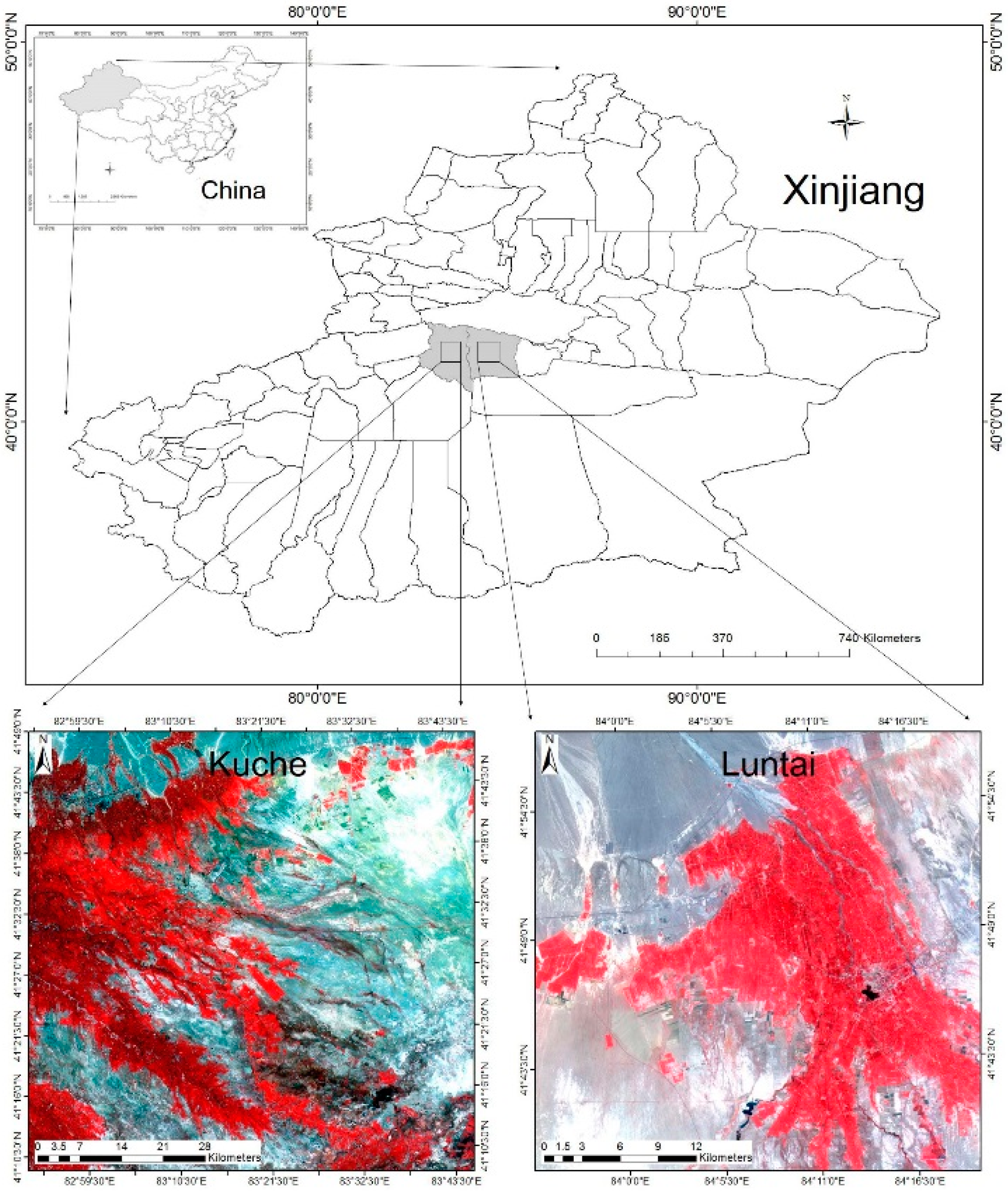
Figure 1. Locations of the study areas.
Ijerph 12 09920 g001

2. Study Area and Data Preparation

2.1. Study Area

Two counties located in Xinjiang Province, China, were selected as the study areas (Figure 1). The first county, Kuche, Aksu City, Xinjiang Province, China, is located at 40°46′–42°35′ N, 82°35′–84°17′ E. The second county, Luntai, Bayinguoleng Mongolian Autonomous Prefecture, Xinjiang Province, China, is located at 41°05′–42°32′ N, 83°38′–85°25′ E. Both counties are located in the south of the middle Tianshan Mountain and the north of Tarim Basin and belong to a warm temperate zone, with a continental arid climate. The north of both counties is mountainous, while the central and southern regions consist of plains. The main landforms of both counties are plains, which are mainly devoted to agriculture, cities and deserts.

2.2. Data and Pre-Processing

Three HJ CCD datasets, six GF-1 wide field of view camera (WFV) datasets and six MODIS surface reflectance datasets were used in this study (Table 1). All of these data were acquired during clear sky conditions and are of good quality.
Table 1. Images used in this research.
Study AreaAcquisition DatePath/Row
HJ-1 CCDGF-1 WFV
Kuche03/10/201341/6458/173
07/10/201342/6456/174
15/10/201345/6458/173
Luntai03/10/201341/6458/167
07/10/201342/6456/168
15/10/201345/6456/168

2.2.1. HJ-1 CCD Data

The HJ satellite constellation consists of two satellites (HJ-1-A and HJ-1-B), and was launched on 6 September 2008. HJ-1-A is equipped with a CCD camera and a hyperspectral imager (HSI). HJ-1-B is equipped with a CCD camera and an infrared camera (IRS). The HJ satellite constellation can image the entire Earth at two-day intervals. Table 2 lists the sensors’ parameters for the HJ satellite constellation.
Three HJ CCD datasets were downloaded from the China Centre for Resources Satellite Data and Application (http://www.cresda.com/n16/index.html). These data were atmospherically corrected using the Fast Line-of-Sight Atmospheric Analysis of Spectral Hypercubes (FLAASH) Atmospheric Correction Model in the ENVI 5.0 software. The three HJ CCD datasets were then georeferenced using a second-order polynomial warping approach based on the selection of 45 ground control points (GCPs) from a 1:10,000 topographic map by the nearest neighbour resampling method, with a position error of within 0.67 HJ CCD pixels.
Table 2. Parameters for HJ satellite constellation sensors.
SatelliteSensorBandBandwidth (nm)Resolution (m)Width (km)Return Cycle (Days)
HJ-1-ACCD1430–520307004
2520–600
3630–690
4760–900
HSI128 bands450–950100504
HJ-1-BCCD1430–520307004
2520–600
3630–690
4760–900
IRS5750–11001507204
61550–1750
73500–3900
810500–12500300

2.2.2. GF-1 WFV Data

The GF-1 satellite is a Chinese sun-synchronous, high-resolution satellite. It was launched on 26 April 2013. The GF-1 satellite is equipped with two types of sensors: two panchromatic multispectral sensors (MPS) and four WFV cameras. It can acquire panchromatic images with a resolution of 2 m, and multispectral images at a resolution of 8 m or 16 m. Table 3 lists the sensors’ parameters for the GF-1 satellite.
Table 3. Parameters for the GF-1 satellite sensors.
SensorBandwidth (nm)Resolution (m)Width (km)Return Cycle (Days)
MPS450–9002604 (side swing)
41 (no side swing)
430–5208
520–600
630–690
760–900
WFV430–520168004
520–600
630–690
760–900
Six GF-1 WFV datasets, provided by the GF Satellite Application Technology Centre, Institute of Remote Sensing and Digital Earth, Chinese Academy of Sciences, were used in this study (Table 1). These data were orthorectified with ENVI 5.0 software, using rational polynomial coefficients (RPC) with a Digital Elevation Model (DEM) and 36 GCPs selected from a 1:10,000 topographic map. The data were then atmospherically corrected using the FLAASH Atmospheric Correction Model with the ENVI 5.0 software provided by Esri China Information Technology Co., Ltd., Beijing, China.

2.2.3. MODIS Data

Three 500 m resolution daily MODIS surface reflectance products (MOD09GA) and three 250 m resolution daily MODIS surface reflectance products (MOD09GQ) were used in this study (Table 1). These MODIS images were reprojected from the native sinusoidal projection onto the UTM-WGS84 reference system, and were resized to the selected study area using MODIS Reprojection Tool (MRT) software. These MODIS data were then georeferenced using a second-order polynomial warping approach based on the selection of 28 or 32 GCPs from 500 m or 250 m GF-1 WFV images, respectively, with a nearest neighbour resampling method that has a position error of within 0.53 and 0.67 GF-1 WFV pixels, respectively. The 500 m and 250 m GF-1 WFV images were resized from georeferenced GF-1 WFV images using the pixel aggregate resampling method.

3. Methods

3.1. Model Introduction

3.1.1. ESTARFM

ESTARFM was proposed to improve the STARFM algorithm for the accurate prediction of surface reflectance in heterogeneous landscapes using the observed reflectance trend between two points in time and spectral unmixing theory [38]. According to the linear mixture model, the changes in coarse-resolution reflectance from t0 to tk can be expressed as:
R ( t k ) R ( t 0 ) = i = 1 M f i a ( r ( t k ) r ( t 0 ) )
where R ( t k ) and R ( t 0 ) are the coarse-resolution reflectances from time t0 to tk, r ( t k ) and r ( t 0 ) are the fine-resolution reflectances from time t0 to tk, M is the total number of endmembers, f i is the fraction of the i-th land type and a is the sensor calibration coefficient. ESTARFM assumes that thechange in the reflectance of each land type is linear with time:
r ( t k ) = h k × Δ t + r ( t 0 )
where Δ t = t k t 0 and hk is the rate of change of the k-th endmember, which was assumed to be constant from time t0 to tk. Then, Equations (1) and (2) can be rewritten as:
Δ t = ( r ( t k ) r ( t 0 ) ) h k
R ( t k ) R ( t 0 ) = Δ t i = 1 M f i h i a
Substituting Equation (3) into Equation (4), the ratio, vk, of the change in reflectance for the k-th endmember to the change in reflectance for a coarse pixel can be described as:
r ( t k ) r ( t 0 ) R ( t k ) R ( t 0 ) = h k i = 1 M f i h i a = v k
Equation (5) can be rewritten as:
r ( x , y , t k ) = r ( x , y , t 0 ) + v k × ( R ( x , y , t k ) R ( x , y , t 0 ) )
where (x,y) is the position of the target pixels.
By introducing additional information from the neighbouringpixels to reduce the influence of land cover changes, surface heterogeneity and solar geometrybi-directional reflectance distribution function (BRDF) changes, a weighted ESTARFM can be determined as Equation (7):
r ( x , y , t k ) = r ( x i , y j , t 0 ) + i = 1 w j = 1 w k = 1 n W i j k × v i j k ( R ( x i , y j , t k ) R ( x i , y j , t 0 ) )
where w is the size of the search window; W i j k is the weight determined by the spectral difference S i j k and the temporal difference T i j k between the fine- and low-resolution data, and by the location distance D i j k between the target pixel and the candidate pixel; k is the number of pixels (xi,yj) in window w. These parameters are calculated as follows:
W i = ( 1 / D i ) / i = 1 n ( 1 / D i )
D i = ( 1 + S i ) × d i
d i = 1 + ( x x i ) 2 + ( y y i ) 2 / ( w / 2 )
S i = E [ ( r i E ( r i ) ) × ( R i E ( R i ) ) ] D ( r i ) × D ( R i )

3.1.2. STDFA

STDFA is based on a linear mixing model that assumes the reflectance of each coarse spatial resolution pixel is a linear combination of the responses of each land cover class contributing to the mixture [49]:
R ( x , y , t ) = i = 0 M f i ( x , y , i ) × r ¯ ( i , t ) + ξ ( x , y , t )
Constraint : i = 0 M f i ( x , y , i ) < 1   and   f i ( x , y , i ) 0     for all .
where r ¯ ( i , t ) is the mean reflectance of land type i at time t and ξ ( x , y , t ) is the residual error term. By inputting the fraction data f i ( x , y , i ) extracted from the land cover map, the mean reflectance for land cover class i can be calculated by solving Equation (12) using the ordinary least squares technique. Then, based on the assumption that the temporal variation properties of each fine-resolution pixel in the same class are constant, the STDFA predicts synthetic high-resolution spatial imagery as follows:
r ( x , y , t k ) = r ( x , y , t 0 ) + r ¯ ( c , t k ) r ¯ ( c , t 0 )

3.2. Model Application

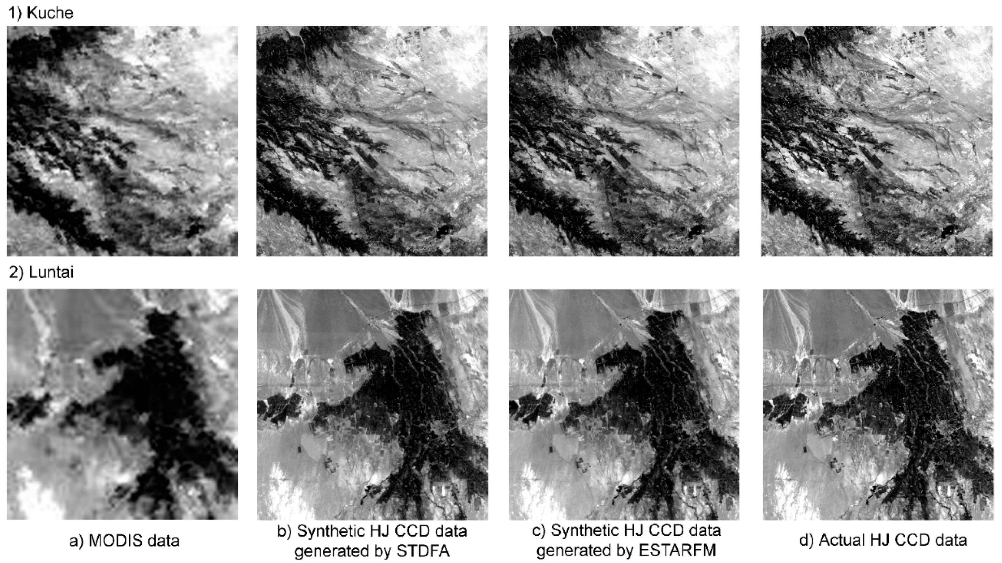
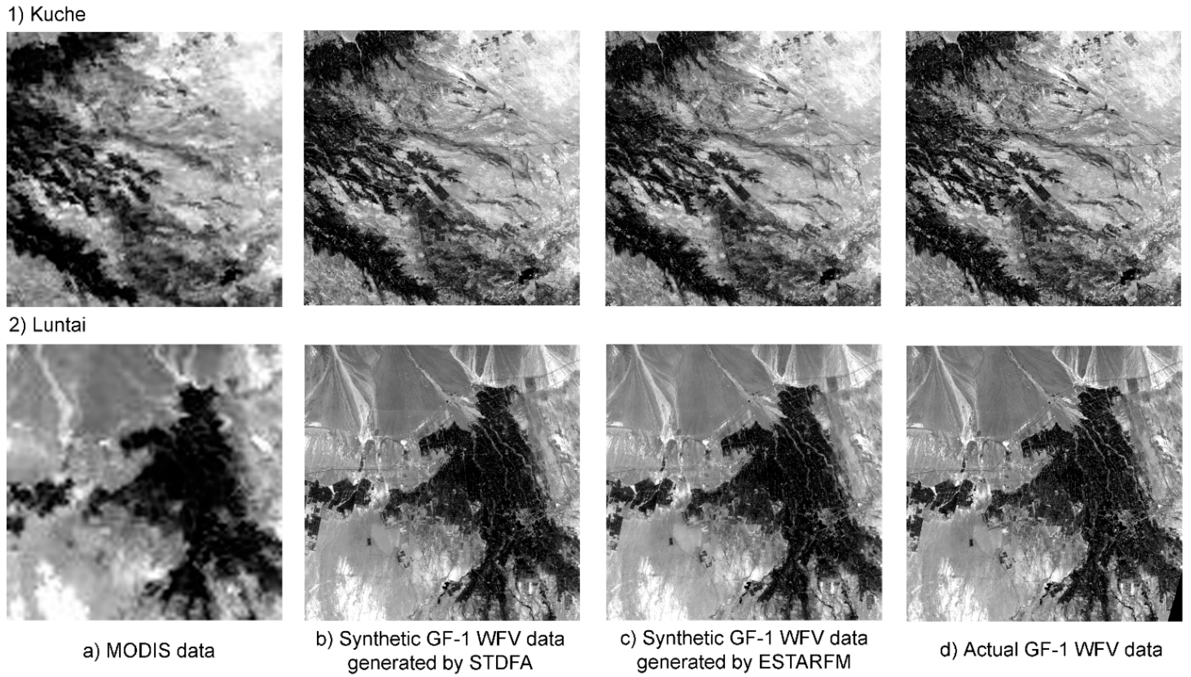
According to Equation (7), three images are needed for ESTARFM: fine-resolution data acquired at time t0, called the base image, and two low-resolution datasets acquired at times t0 and tk, called the time series low-resolution data. Two pairs of fine-resolution and low-resolution datasets acquired at time t0 and time tl are also required to calculate the spectral similarity index. According to Equation (12), three images are needed for STDFA: a fine-resolution dataset acquired at time t0, called the base image, and two low-resolution datasets acquired at times t0 and tk, called the time series low-resolution data. Two fine-resolution datasets acquired at time t0 and time tl are also required for classification. The outputs of ESTARFM and STDFA are synthetic fine-resolution data acquired at time tk. In this study, HJ-1 CCD and GF-1 WFV data acquired on 3 October 2013 were used as the base image. MODIS images acquired on 3 October 2013 and 7 October 2013 were used as the time series low-resolution data. Two pairs, HJ-1 CCD and MODIS data, or GF-1 WFV and MODIS data, acquired on 3 October 2013 and 15 October 2013 were used to calculate the spectral similarity index for ESTARFM. Two HJ-1 CCD or GF-1 WFV datasets, acquired on 3 October 2013 and 15 October 2013, were used for classification in STDFA. The outputs of ESTARFM and STDFA are synthetic HJ-1 CCD and GF-1 WFV data acquired on 7 October 2013.

3.3. Validation of Results

Since the objective of the ESTARFM and STDFA methods was to generate synthetic fine-resolution data, actual HJ-1 CCD and GF-1 WFV data acquired on 7 October 2013 were used to validate the algorithm using the methods proposed by Wu et al. [44]. First, the results were qualitatively evaluated using visual interpretation. The greater the similarity between the synthetic and actual fine-resolution data, the higher the accuracy of the model. Second, the results were quantitatively evaluated using the correlation analysis method. Parameters, such as the correlation coefficient (r), variance (Var), mean absolute difference (MAD), bias and root mean square error (RMSE), were calculated to quantitatively evaluate the precision of these models. A higher value of r and lower variance, MAD, bias and RMSE indicate higher accuracy.

3.4. Accuracy Comparison for the Fusion Results Using 250 m and 500 m MODIS Data

There are two reflectance MODIS data products: MOD09GQ and MOD09GA. Both products can be used in spatial and temporal data fusion, but the question remains as to whether the spatial resolution differences between these two products have an impact on the fusion accuracy. To answer this question, we applied STDFA and ESTARFM using MOD09GQ data in Kuche and Luntai, and compared the fusion results with results obtained using MOD09GA data. The correlation analysis method was used to evaluate the similarity of the actual fine-resolution data and the synthetic fine-resolution data generated by inputting MOD09GQ and MOD09GA. By comparing the r, variance, MAD, bias and RMSE we can analyse the influence of spatial resolution differences for these two data products.

3.5. Comparison of Actual NDVI and NDVI Calculated Using Synthetic Data

The synthetic red- and near infrared (NIR)-band data were generated using STDFA and ESTARFM in Kuche and Luntai, allowing Normalized Different Vegetation Index (NDVI) images in these two study areas to be calculated. The correlation analysis method was then used to evaluate the similarity of the NDVI image calculated from synthetic fine-resolution data and the NDVI image calculated from actual fine-resolution data.

4. Results

4.1. HJ and MODIS Fusion Results

By inputting a base HJ CCD image, two days of MOD09GA data and two days of multi-spectral HJ CCD images, a synthetic multi-spectral HJ CCD image was generated by STDFA. By inputting a base HJ CCD image, two days of multi-spectral MOD09GA data and two days of multi-spectral MODIS data and HJ CCD datasets, a synthetic multi-spectral HJ CCD image was also generated by ESTARFM. These synthetic multi-spectral HJ CCD images contained four bands, including blue, green, red and NIR. Figure 2a shows the actual observed MODIS surface reflectance in the red band acquired on 7 October 2013 in Kuche and Luntai. Figure 2b, c show the synthetic surface reflectance imagery in the red band generated by STDFA and ESTARFM, respectively, for the two study areas. Figure 2d shows the actual observed HJ CCD red-band surface reflectance acquired on 7 October 2013 in Kuche and Luntai.
Figure 2. Comparison of MODIS, HJ CCD and synthetic data generated by the ESTARFM and STDFA acquired on 7 October 2013: (a) MODIS data; (b) synthetic HJ CCD data generated by STDFA; (c) synthetic HJ CCD data generated by ESTARFM; (d) actual HJ CCD data.
Ijerph 12 09920 g002
The actual high spatial resolution data acquired on 7 October 2013 was used to evaluate the accuracy of these models. Through visual interpretation, we found that the synthetic and actual HJ CCD data are very similar, and were hard to distinguish between with the naked eye. Table 4 shows the results of the quantitative evaluation using the correlation analysis method. From Table 4, we can see that both STDFA and ESTARFM can generate synthetic HJ CCD data that are very similar to actual HJ CCD data, with r values greater than 0.8989. STDFA showed a slightly better performance than ESTARFM for Luntai and Kuche.
Table 4. Results of the correlation analysis between synthetic and actual HJ CCD data.
Kuche
ParametersSTDFAESTARFM
BlueGreenRedNIRBlueGreenRedNIR
r0.9493 0.9642 0.9759 0.9231 0.9463 0.9601 0.9714 0.8989
Var0.0001 0.0002 0.0002 0.0001 0.0002 0.0002 0.0002 0.0002
MAD0.0091 0.0104 0.0096 0.0086 0.0093 0.0110 0.0106 0.0100
RMSE0.0494 0.0422 0.0166 0.0364 0.0425 0.0305 0.0218 0.0177
bias−0.0479 −0.0399 −0.0109 −0.0344 −0.0406 −0.0270 −0.0169 −0.0115
Luntai
ParametersSTDFAESTARFM
BlueGreenRedNIRBlueGreenRedNIR
r0.9591 0.9640 0.9761 0.9608 0.9585 0.9598 0.9724 0.9475
Var0.0002 0.0002 0.0002 0.0001 0.0002 0.0003 0.0002 0.0002
MAD0.0098 0.0114 0.0102 0.0081 0.0099 0.0119 0.0108 0.0108
RMSE0.0461 0.0404 0.0336 0.0226 0.0466 0.0344 0.0275 0.0175
bias−0.0441 −0.0375 −0.0308 −0.0197 −0.0446 −0.0305 −0.0235 −0.0098

4.2. GF and MODIS Fusion Results

By inputting a base GF-1 WFV image, two days of MOD09GA data and two days of multi-spectral GF-1 WFV images, a synthetic multi-spectral GF-1 WFV image was generated by STDFA. By inputting a base GF-1 WFV image, two days of multi-spectral MOD09GA data and two days of multi-spectral MODIS data and GF-1 WFV datasets, a synthetic multi-spectral GF-1 WFV image was also generated by ESTARFM. These synthetic multi-spectral GF-1 WFV images contained four bands, including blue, green, red and NIR. Figure 3a shows the actual observed MODIS surface reflectance in the red band acquired on 7 October 2013 in Kuche and Luntai. Figure 3b, c show the synthetic GF-1 WFV surface reflectance imagery in the red band generated by STDFA and ESTARFM, respectively, for the two study areas. Figure 3d shows the actual observed GF-1 WFV red-band surface reflectance acquired on 7 October 2013 in Kuche and Luntai.
Through visual interpretation, we found that the synthetic and actual GF-1 WFV data are very similar and were not distinguishable with the naked eye. Table 5 shows the results of the quantitative evaluation using the correlation analysis method. From Table 5, we also find that both STDFA and ESTARFM can generate synthetic GF-1 WFV data that are very similar to actual GF-1 WFV data, with r values greater than 0.8643. ESTARFM performed slightly better than STDFA in Kuche, while the accuracies of these two methods were very similar in Luntai.
Figure 3. Comparison of MODIS, GF-1 WFV and synthetic data generated by ESTARFM and STDFA acquired on 7 October 2013: (a) MODIS data; (b) synthetic GF-1 WFV data generated by STDFA; (c) synthetic GF-1 WFV data generated by ESTARFM; (d) actual GF-1 WFV data.
Ijerph 12 09920 g003
Table 5. Results of the correlation analysis between synthetic and actual GF-1 WFV data.
Kuche
ParametersSTDFAESTARFM
BlueGreenRedNIRBlueGreenRedNIR
r0.9658 0.9687 0.9778 0.9513 0.9669 0.9705 0.9790 0.9563
Var0.0001 0.0001 0.0002 0.0001 0.0001 0.0001 0.0001 0.0001
MAD0.0079 0.0089 0.0093 0.0081 0.0076 0.0085 0.0088 0.0078
RMSE0.0264 0.0279 0.0254 0.0222 0.0220 0.0209 0.0180 0.0168
bias−0.0240 −0.0252 −0.0222 −0.0188 −0.0193 −0.0174 −0.0135 −0.0124
Luntai
ParametersSTDFAESTARFM
BlueGreenRedNIRBlueGreenRedNIR
r0.9334 0.9199 0.9315 0.8654 0.9338 0.9251 0.9314 0.8643
Var0.0002 0.0003 0.0004 0.0006 0.0002 0.0003 0.0004 0.0006
MAD0.0083 0.0105 0.0102 0.0098 0.0082 0.0096 0.0102 0.0105
RMSE0.0287 0.0245 0.0287 0.0317 0.0272 0.0274 0.0261 0.0289
bias−0.0249 −0.0165 −0.0211 −0.0195 −0.0231 −0.0211 −0.0175 −0.0141

4.3. Accuracy Comparison for the Fusion Results Using 250 m and 500 m MODIS Data

To analyse the influence of spatial resolution differences, we applied STDFA and ESTARFM using MOD09GQ data in Kuche and Luntai, and compared the fusion results with the results obtained using MOD09GA data. Table 6 shows the results of the correlation analysis between synthetic data generated using MOD09GQ data and actual data. Comparing Table 6, Table 4 and Table 5, we find that the spatial resolution differences had more impact on the fusion accuracy for ESTARFM than for STDFA in these two study areas. This is mainly because the MODIS reflectance was directly used to calculate the fine reflectance in ESTARFM, while it was used to calculate the mean reflectance of each land cover type in STDFA.
Table 6. Results of the correlation analysis between synthetic data generated using MOD09GA data and actual data.
GF-1 WFV
Study AreaKucheLuntai
ParametersSTDFAESTARFMSTDFAESTARFM
RedNIRRedNIRRedNIRRedNIR
r0.9785 0.9489 0.9776 0.9505 0.9306 0.8673 0.9302 0.8624
Var0.0001 0.0001 0.0001 0.0001 0.0004 0.0006 0.0004 0.0006
MAD0.0091 0.0081 0.0089 0.0084 0.0099 0.0096 0.0108 0.0108
RMSE0.0253 0.0269 0.0192 0.0186 0.0286 0.0314 0.0248 0.0279
bias−0.0223 −0.0243 −0.0151 −0.0142 −0.0212 −0.0193 −0.0152 −0.0116
HJ CCD
Study AreaKucheLuntai
ParametersSTDFAESTARFMSTDFAESTARFM
RedNIRRedNIRRedNIRRedNIR
r0.9783 0.9186 0.9690 0.8818 0.9737 0.9619 0.9533 0.9728
Var0.0001 0.0001 0.0002 0.0002 0.0002 0.0001 0.0002 0.0002
MAD0.0093 0.0089 0.0111 0.0108 0.0097 0.0080 0.0102 0.0108
RMSE0.0360 0.0363 0.0219 0.0174 0.0335 0.0223 0.0173 0.0277
bias−0.0338 −0.0343 −0.0167 −0.0099 −0.0309 −0.0194 −0.0109 −0.0237

4.4. Comparison of Actual NDVI and NDVI Calculated Using Synthetic Data

NDVI images calculated using actual data were used to evaluate the quality of the synthetic NDVI images. Table 7 shows the results of the correlation analysis between synthetic and actual NDVI data. From Table 7, we find that the NDVI data calculated using synthetic data generated by ESTARFM were more similar to actual NDVI than the NDVI data calculated using synthetic data generated by STDFA.
Table 7. Result of the correlation analysis between synthetic and actual NDVI data.
ParametersGF-1 WFVHJ CCD
KucheLuntaiKucheLuntai
STDFAESTARFMSTDFAESTARFMSTDFAESTARFMSTDFAESTARFM
r0.9798 0.9803 0.9703 0.9742 0.9686 0.9722 0.9769 0.9801
Var0.0012 0.0011 0.0017 0.0016 0.0011 0.0011 0.0017 0.0016
MAD0.0264 0.0236 0.0266 0.0259 0.0252 0.0255 0.0318 0.0315
RMSE0.0463 0.0372 0.0479 0.0461 0.0416 0.0405 0.0580 0.0568
bias0.0300 0.0180 0.0247 0.0226 −0.0247 0.0223 0.0412 0.0400

5. Discussion

This study applied and demonstrated the use of ESTARFM and STDFA in combining HJ CCD, GF-1 WFV and MODIS data to generate high spatial resolution data. Although the data quality of HJ CCD data is lower than Landsat data, both the ESTARFM and STDFA algorithms can generate daily synthetic high spatial resolution data accurately, with r values higher than 0.8643 and RMSEs lower than 0.0360. As the MODIS sensor can acquire daily images, ESTARFM and STDFA can be used to enhance the proportion of useful HJ CCD and GF-1 WFV data. For example, the proportion of useful MODIS data in Luntai for 2013 is 48.49%, while the proportions of useful HJ CCD data and useful GF-1 WFV data are 15.07% and 10.29%, respectively. Owing to the high proportion of useful data, this method is potentially useful for high spatial resolution environmental process monitoring, and can be applied in natural resource damage assessments and environmental policy and management. However, there are some issues should be addressed in the application of this method:
(1) Influence of the satellite data quality. The test areas for the HJ-MODIS fusion and the GF-MODIS fusion in Kuche were the same, while the test area for the GF-MODIS fusion was a little larger than the area for the HJ-MODIS fusion in Luntai. Therefore, we can only analyse the influence of the satellite data quality on the data fusion for the Kuche area. As an early Chinese moderate-resolution satellite, the quality of HJ satellite data is lower than the quality of GF-1 satellite data. The position error of HJ CCD data is greater than 1 km, while the position error of GF-1 WFV data is less than 100 m. Furthermore, the SNR of HJ CCD data is much lower than the SNR of GF-1 WFV data. Table 6 lists the differences between Table 5 and Table 4, showing the influence of the sensor differences on the model accuracy. From Table 8, we can see that the influence of the sensor differences for STDFA is less significant than for ESTARFM. This is because STDFA had better noise immunity. Similar results were found for the fusion of ASTER and MODIS land surface temperature products [46].
Table 8. Influence of sensor differences on model accuracy.
ParametersSTDFAESTARFM
BlueGreenRedNIRBlueGreenRedNIR
r0.0165 0.0045 0.0018 0.0283 0.0206 0.0104 0.0077 0.0574
Var0.0000 0.0000 0.0000 0.0000 0.0000 −0.0001 0.0000 0.0000
MAD−0.0012 −0.0015 −0.0003 −0.0005 −0.0017 −0.0025 −0.0018 −0.0022
RMSE−0.0230 −0.0143 0.0088 −0.0142 −0.0205 −0.0096 −0.0038 −0.0009
bias−0.0238 −0.0147 0.0113 −0.0156 −0.0213 −0.0096 −0.0034 0.0009
(2) Influence of bidirectional reflectance distribution function (BRDF) changes. For different data acquisition dates, the solar and satellite azimuth and zenith angles are different (Table 9). This leads to changes in the BRDF and hence in the information received by the sensor. More seriously, this could lead to differences in the shadow direction and length for the same object on different dates. 
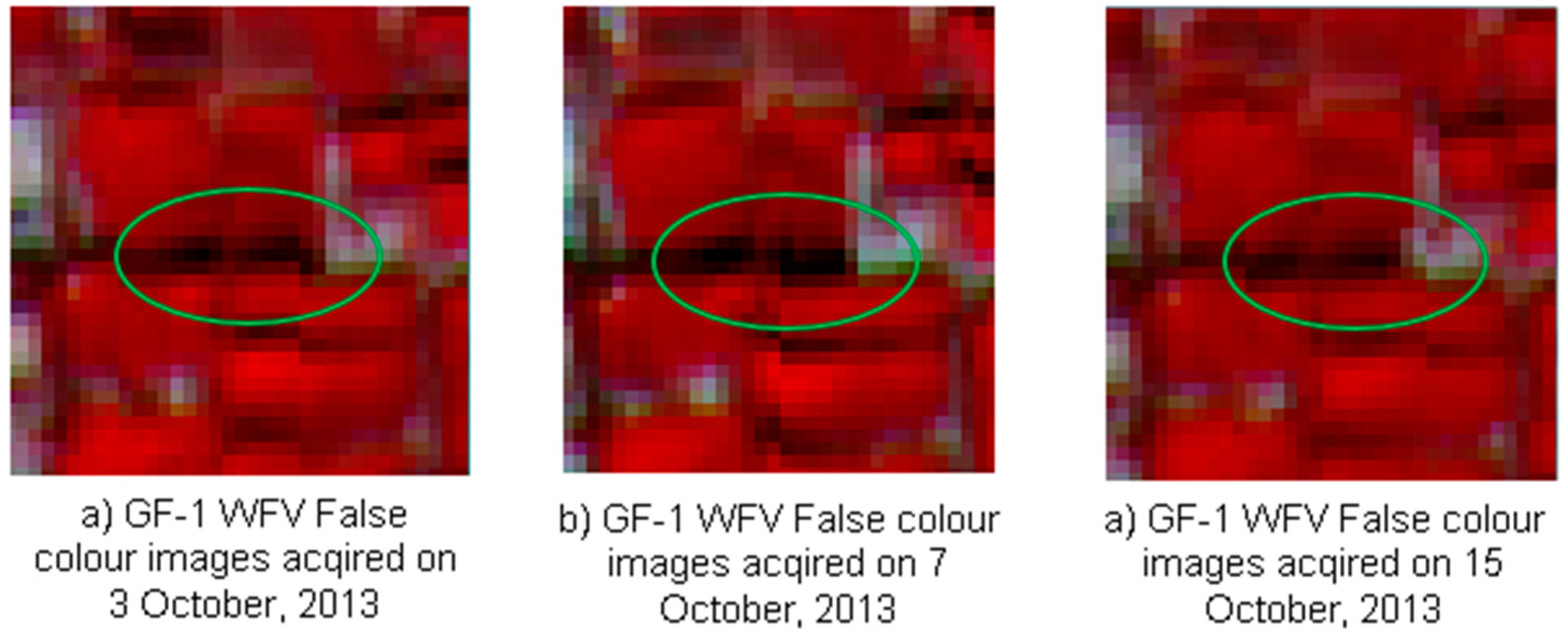
Figure 4 shows an example of the difference in the shadow direction and length for trees on 3 October 2013, 7 October 2013 and 15 October 2013 recorded by the GF-1 WFV sensor. In the shaded area, the differences of reflectance in the NIR band between actual and synthetic GF-1 WFV data can reach 0.0676 for STDFA and 0.0638 for ESTARFM. However, in the unshaded area, the differences of reflectance in the NIR band between actual and synthetic GF-1 WFV data were only 0.0078 for STDFA and 0.0153 for ESTARFM. Therefore, we conclude that further study is required regarding this problem.
Table 9. Sensors and solar azimuth information from GF-1 WFV data.
Image Information3 October 20137 October 201315 October 2013
Receive Time (local time)13:34:1113:33:2413:31:47
Solar Azimuth166.147166.601167.415
Solar Zenith42.411740.922537.9947
Satellite Azimuth235.912121.314106.892
Satellite Zenith89.183888.338484.7204
Figure 4. An example of the difference in shadow direction and length.
Ijerph 12 09920 g004
(3) The ESTARFM and STDFA algorithms were proposed to enhance the temporal resolution of high spatial resolution data. High spatial and temporal remote sensing data can be generated using these methods. However, spectral fusion was not considered for these methods. Therefore, these methods can only be used for spatial and temporal fusion, and we recommend using the spectral fusion method in the future to improve the spectral resolution of sensors [50]. In addition, it has been proposed that these methods could be used to fuse optical images that are easily affected by cloudy weather. Although these methods can improve the proportion of useful data, a significant proportion of the data will be polluted by cloud. The development of an optical and radar data fusion algorithm is therefore an important direction for multi-source remote sensing data studies.

6. Conclusions

In two study areas located in Xinjiang Province, China, the ESTARFM and STDFA methods were applied to combine HJ CCD, GF-1 WFV and MODIS reflectance data. We found the following conclusions:
(1)
Both ESTARFM and STDFA methods can be applied to combine HJ CCD and MODIS reflectance data, and GF-1 WFV and MODIS reflectance data. Synthetic HJ CCD data are very similar to actual HJ CCD data, with r values greater than 0.8989 generated using these two methods. Synthetic GF-1 WFV data are very similar to actual GF-1 WFV data, generating r values greater than 0.8643.
(2)
The accuracy differences between the fusion of HJ CCD and MODIS data and the fusion of GF-1 WFV and MODIS data were lower for STDFA than for ESTARFM. STDFA had better noise immunity than ESTARFM.
(3)
The spatial resolution differences between MOD09GQ and MOD09GA had a more significant impact on the fusion accuracy for ESTARFM than for STDFA.
(4)
Synthetic red- and NIR-band data generated by ESTARFM are more suitable for the calculation of NDVI than the data generated by STDFA.

Acknowledgments

This work was supported by the National Natural Science Foundation of China (41301390), the National Science and Technology Major Project (2014AA06A511), the Major State Basic Research Development Program of China (2013CB733405, 2010CB950603) and the National Science and Technology Major Project of China. The funders had no role in choosing the study design, in the collection, analysis and interpretation of the data, in the writing of the report, or in the decision to submit the article for publication.

Author Contributions

Mingquan Wu, Wenjiang Huang, Zheng Niu and Changyao Wang conceived and designed the experiments. Mingquan Wu performed the experiments and the manuscript draft. Wenjiang Huang, Zheng Niu and Changyao Wang revised the manuscript draft. All authors read and approved the final version.

Conflicts of Interest

The authors declare no conflict of interest.

References

  1. Politi, E.; Cutler, M.E.J.; Rowan, J.S. Using the NOAA Advanced Very High Resolution Radiometer to characterise temporal and spatial trends in water temperature of large European lakes. Remote Sens. Environ. 2012, 126, 1–11. [Google Scholar] [CrossRef] [Green Version]
  2. Maisongrande, P.; Duchemin, B.; Dedieu, G. VEGETATION/SPOT: An operational mission for the Earth monitoring; presentation of new standard products. Int. J. Remote Sens. 2004, 25, 9–14. [Google Scholar] [CrossRef]
  3. Salomonson, V.V.; Barnes, W.L.; Maymon, P.W.; Montgomery, H.E.; Ostrow, H. MODIS: Advanced facility instrument for studies of the earth as a system. IEEE Trans. Geosci. Remote Sens. 1992, 145–153. [Google Scholar] [CrossRef]
  4. Zhou, H.; Aizen, E.; Aizen, V. Deriving long term snow cover extent dataset from AVHRR and MODIS data: Central Asia case study. Remote Sens. Environ. 2013, 136, 146–162. [Google Scholar] [CrossRef]
  5. Yagoub, H.; Belbachir, A.H.; Benabadji, N. Detection and mapping vegetation cover based on the Spectral Angle Mapper algorithm using NOAA AVHRR data. Adv. Space Res. 2014, 53, 1686–1693. [Google Scholar] [CrossRef]
  6. Shaoa, Y.; Campbell, J.B.; Taff, G.N.; Zheng, B.J. An analysis of cropland mask choice and ancillary data for annual corn yield forecasting using MODIS data. Int. J. Appl. Earth Obs. 2015, 38, 78–87. [Google Scholar] [CrossRef]
  7. Zhang, G.; Xiao, X.; Dong, J.; Kou, W.; Jin, C.; Qin, Y.; Zhou, Y.; Wang, J.; Menarguez, M.A.; Biradar, C. Mapping paddy rice planting areas through time series analysis of MODIS land surface temperature and vegetation index data. ISPRS J. Photogramm. Remote Sens. 2015, 106, 157–171. [Google Scholar] [CrossRef]
  8. Mao, D.H.; Wang, Z.M.; Luo, L.; Ren, C.Y. Integrating AVHRR and MODIS data to monitor NDVI changes and their relationships with climatic parameters in Northeast China. Int. J. Appl. Earth Obs. 2012, 18, 528–536. [Google Scholar] [CrossRef]
  9. Maignan, F.; Bréon, F.-M.; Bacour, C.; Demarty, J.; Poirson, A. Interannual vegetation phenology estimates from global AVHRR measurements Comparison with in situ data and applications. Remote Sens. Environ. 2008, 112, 496–505. [Google Scholar] [CrossRef]
  10. Fensholt, R.; Rasmussen, K.; Nielsen, T.T.; Mbow, C. Evaluation of earth observation based long term vegetation trends—Intercomparing NDVI time series trend analysis consistency of Sahel from AVHRR GIMMS, Terra MODIS and SPOT VGT data. Remote Sens. Environ. 2009, 113, 1886–1898. [Google Scholar] [CrossRef]
  11. Ruiz, J.A.M.; Riaño, D.; Arbelo, M.; French, N.H.F.; Ustin, S.L.; Whiting, M.L. Burned area mapping time series in Canada (1984–1999) from NOAA-AVHRR LTDR: A comparison with other remote sensing products and fire perimeters. Remote Sens. Environ. 2012, 117, 407–414. [Google Scholar] [CrossRef]
  12. Stellmes, M.; Udelhoven, T.; Röder, A.; Sonnenschein, R.; Hill, J. Dryland observation at local and regional scale—Comparison of Landsat TM/ETM+ and NOAA AVHRR time series. Remote Sens. Environ. 2010, 114, 2111–2125. [Google Scholar] [CrossRef]
  13. Gehlot, S.; Minnett, P.J.; Stammer, D. Impact of Sahara dust on solar radiation at Cape Verde Islands derived from MODIS and surface measurements. Remote Sens. Environ. 2015, 166, 154–162. [Google Scholar] [CrossRef]
  14. Hardtke, L.A.; Blanco, P.D.; Valle, H.F.; Metternicht, G.I.; Sione, W.F. Semi-automated mapping of burned areas in semi-arid ecosystems using MODIS time-series imagery. Int. J. Appl. Earth Obs. 2015, 38, 25–35. [Google Scholar] [CrossRef]
  15. Mehta, M. A study of aerosol optical depth variations over the Indian region using thirteen years (2001–2013) of MODIS and MISR Level 3 data. Atmos. Environ. 2015, 109, 161–170. [Google Scholar] [CrossRef]
  16. Hamer, M.S.; Kloog, I.; Koutrakis, P.; Strawa, A.W.; Chatfield, R.; Cohen, A.; Ridgway, W.L.; Broday, D.M. Assessment of PM2.5 concentrations over bright surfaces using MODIS satellite observations. Remote Sens. Environ. 2015, 163, 180–185. [Google Scholar] [CrossRef]
  17. Li, Y.J.; Xue, Y.; Leeuw, G.D.; Li, C.; Yang, L.; Hou, T.; Marir, F. Retrieval of aerosol optical depth and surface reflectance over land from NOAA AVHRR data. Remote Sens. Environ. 2013, 133, 1–20. [Google Scholar] [CrossRef]
  18. Ayana, E.K.; Worqlul, A.W.; Steenhuis, T.S. Evaluation of streamwater quality data generated from MODIS images in modeling total suspended solid emission to a freshwater lake. Sci. Total Environ. 2015, 523, 170–177. [Google Scholar] [CrossRef] [PubMed]
  19. Zhang, X.Y. Reconstruction of a complete global time series of daily vegetation index trajectory from long-term AVHRR data. Remote Sens. Environ. 2015, 156, 457–472. [Google Scholar] [CrossRef]
  20. Leckie, D. Advances in remote sensing technologies for forest survey and management. Can. J. For. Res. 1990, 21, 464–483. [Google Scholar] [CrossRef]
  21. Han, X.X.; Chen, X.L.; Feng, L. Four decades of winter wetland changes in Poyang Lake based on Landsat observations between 1973 and 2013. Remote Sens. Environ. 2015, 156, 426–437. [Google Scholar] [CrossRef]
  22. Ottinger, M.; Kuenzer, C.; Liu, G.; Wang, S.; Dech, S. Monitoring land cover dynamics in the Yellow River Delta from 1995 to 2010 based on Landsat 5 TM. Appl. Geogr. 2013, 44, 53–68. [Google Scholar] [CrossRef]
  23. Potapov, P.V.; Turubanova, S.A.; Tyukavina, A.; Krylov, A.M.; McCarty, J.L.; Radeloff, V.C.; Hansen, M.C. Eastern Europe’s forest cover dynamics from 1985 to 2012 quantified from the full Landsat archive. Remote Sens. Environ. 2015, 159, 28–43. [Google Scholar] [CrossRef]
  24. Griffiths, P.; Kuemmerle, T.; Baumann, M.; Radeloff, V.V.; Abrudan, I.V.; Lieskovsky, J.; Munteanu, C.; Ostapowicz, K.; Hostert, P. Forest disturbances, forest recovery, and changes in forest types across the Carpathian ecoregion from 1985 to 2010 based on Landsat image composites. Remote Sens. Environ. 2014, 151, 72–88. [Google Scholar] [CrossRef]
  25. DeVries, B.; Verbesselt, J.; Kooistra, L.; Herold, M. Robust monitoring of small-scale forest disturbances in a tropical montane forest using Landsat time series. Remote Sens. Environ. 2015, 161, 107–121. [Google Scholar] [CrossRef]
  26. Tulbure, M.G.; Broich, M. Spatiotemporal dynamic of surface water bodies using Landsat time-series data from 1999 to 2011. ISPRS J. Photogramm. Remote Sens. 2013, 79, 44–52. [Google Scholar] [CrossRef]
  27. Dong, J.; Xiao, X.; Kou, W.; Qin, Y.; Zhang, J.; Li, L.; Jin, C.; Zhou, Y.; Wang, J.; Biradar, C.; et al. Tracking the dynamics of paddy rice planting area in 1986–2010 through time series Landsat images and phenology-based algorithms. Remote Sens. Environ. 2015, 160, 99–113. [Google Scholar] [CrossRef]
  28. Xu, H.Q.; Huang, S.L.; Zhang, T.J. Built-up land mapping capabilities of the ASTER and Landsat ETM+ sensors in coastal areas of southeastern China. Adv. Space Res. 2013, 52, 1437–1449. [Google Scholar] [CrossRef]
  29. Melaas, E.K.; Friedl, M.A.; Zhu, Z. Detecting interannual variation in deciduous broadleaf forest phenology using Landsat TM/ETM+ data. Remote Sens. Environ. 2013, 132, 176–185. [Google Scholar] [CrossRef]
  30. Minn, M.; Cutts, B.B.; Greenberg, J.A.; Pavlovic, N.; Fraterrigo, J.M.; Turner, V.K. Detection of foreclosure-related landscape management changes using Landsat. Appl. Geogr. 2015, 62, 217–224. [Google Scholar] [CrossRef]
  31. Rufin, P.; Müller, H.; Pflugmacher, D.; Hostert, P. Land use intensity trajectories on Amazonian pastures derived from Landsat time series. Int. J. Appl. Earth Obs. 2015, 41, 1–10. [Google Scholar] [CrossRef]
  32. Gao, F.; Masek, J.; Schwaller, M.; Hall, F. On the blending of the Landsat and MODIS surface reflectance: Predicting daily Landsat surface reflectance. IEEE Trans. Geosci. Remote Sens. 2006, 44, 2207–2218. [Google Scholar]
  33. Hilker, T.; Wulder, M.A.; Coops, N.C.; Linke, J.; McDermid, G.; Masek, J.G.; Gao, F.; White, J.C. A new data fusion model for high spatial- and temporal-resolution mapping of forest disturbance based on Landsat and MODIS. Remote Sens. Environ. 2009, 113, 1613–1627. [Google Scholar] [CrossRef]
  34. Liu, H.; Weng, Q.H. Enhancing temporal resolution of satellite imagery for public health studies: A case study of West Nile Virus outbreak in Los Angeles in 2007. Remote Sens. Environ. 2012, 117, 57–71. [Google Scholar] [CrossRef]
  35. Walker, J.J.; Beurs, K.M.; Wynne, R.H.; Gao, F. Evaluation of Landsat and MODIS data fusion products for analysis of dry land forest phonology. Remote Sens. Environ. 2012, 117, 381–393. [Google Scholar] [CrossRef]
  36. Weng, Q.H.; Fua, P.; Gao, F. Generating daily land surface temperature at Landsat resolution by fusing Landsat and MODIS data. Remote Sens. Environ. 2014, 145, 55–67. [Google Scholar] [CrossRef]
  37. Schmidt, M.; Lucas, R.; Bunting, P.; Verbesselt, J.; Armston, J. Multi-resolution time series imagery for forest disturbance and regrowth monitoring in Queensland, Australia. Remote Sens. Environ. 2015, 158, 156–168. [Google Scholar] [CrossRef] [Green Version]
  38. Zhu, X.; Chen, J.; Gao, F.; Chen, X.; Masek, J.G. An enhanced spatial and temporal adaptive reflectance fusion model for complex heterogeneous regions. Remote Sens. Environ. 2010, 114, 2610–2623. [Google Scholar] [CrossRef]
  39. Emelyanova, I.V.; McVicar, T.R.; Niel, T.G.V.; Li, L.T.; van Dijk, A.I.J.M. Assessing the accuracy of blending Landsat–MODIS surface reflectances in two landscapes with contrasting spatial and temporal dynamics: A framework for algorithm selection. Remote Sens. Environ. 2013, 133, 193–209. [Google Scholar] [CrossRef]
  40. Jarihani, A.A.; McVicar, T.R.; Van Niel, T.G.; Emelyanova, I.V.; Callow, J.N.; Johansen, K. Blending Landsat and MODIS data to generate multispectral indices: A comparison of “Index-then-Blend” and “Blend-then-Index” approaches. Remote Sens. 2014, 6, 9213–9238. [Google Scholar] [CrossRef] [Green Version]
  41. Zhukov, B.; Oertel, D.; Lanzl, F.; Reinhackel, G. Unmixing-based multisensor multiresolution image fusion. IEEE T. Geosci. Remote Sens. 1999, 37, 1212–1226. [Google Scholar] [CrossRef]
  42. Maselli, F. Definition of spatially variable spectral end members by locally calibrated multivariate regression analyses. Remote Sens. Environ. 2001, 75, 29–38. [Google Scholar] [CrossRef]
  43. Busetto, L.; Meronib, M.; Colombo, R. Combining medium and coarse spatial resolution satellite data to improve the estimation of sub-pixel NDVI time series. Remote Sens. Environ. 2008, 112, 118–131. [Google Scholar] [CrossRef]
  44. Wu, M.Q.; Niu, Z.; Wang, C.Y.; Wu, C.Y.; Wang, L. Use of MODIS and Landsat time series data to generate high resolution temporal synthetic Landsat data using a spatial and temporal reflectance fusion model. J. Appl. Remote Sens. 2012, 6. [Google Scholar] [CrossRef]
  45. Wu, M.Q.; Wu, C.Y.; Huang, W.J.; Niu, Z.; Wang, C.Y. High-resolution Leaf Area Index estimation from synthetic Landsat data generated by a spatial and temporal data fusion model. Comput. Electron. Agric. 2015, 115, 1–11. [Google Scholar] [CrossRef]
  46. Wu, M.Q.; Li, H.; Huang, W.J.; Niu, Z.; Wang, C.Y. Generating daily high spatial land surface temperatures by combining ASTER and MODIS land surface temperature products for environmental process monitoring. Environ. Sci. Processes Impacts 2015, 17, 1396–1404. [Google Scholar] [CrossRef] [PubMed]
  47. Gevaert, C.M.; García-Haro, J. A comparison of STARFM and an unmixing-based algorithm for Landsat and MODIS data fusion. Remote Sens. Environ. 2015, 156, 34–44. [Google Scholar] [CrossRef]
  48. Quality Evaluation and Analysis of HJ-1B-CCD Images. Available online: http://www.cnki.net/KCMS/detail/detail.aspx?QueryID=2&CurRec=4&recid=&filename=YGXX201205008&dbname=CJFD2012 (accessed on 7 July 2015).
  49. Settle, J.; Drake, N.A. Linear mixing and the estimation of groundcover proportion. Int. J. Remote Sens. 1993, 14, 1159–1177. [Google Scholar] [CrossRef]
  50. Chen, F.; Niu, Z.; Sun, G.Y.; Wang, C.Y.; Teng, J. Using low-spectral-resolution images to acquire simulated hyperspectral images. Int. J. Remote Sens. 2008, 29, 2963–2980. [Google Scholar] [CrossRef]

