
Intraurban and Longitudinal Variability of Classical Pollutants in Kraków, Poland, 2000–2010

Abstract
:1. Introduction
2. Methods
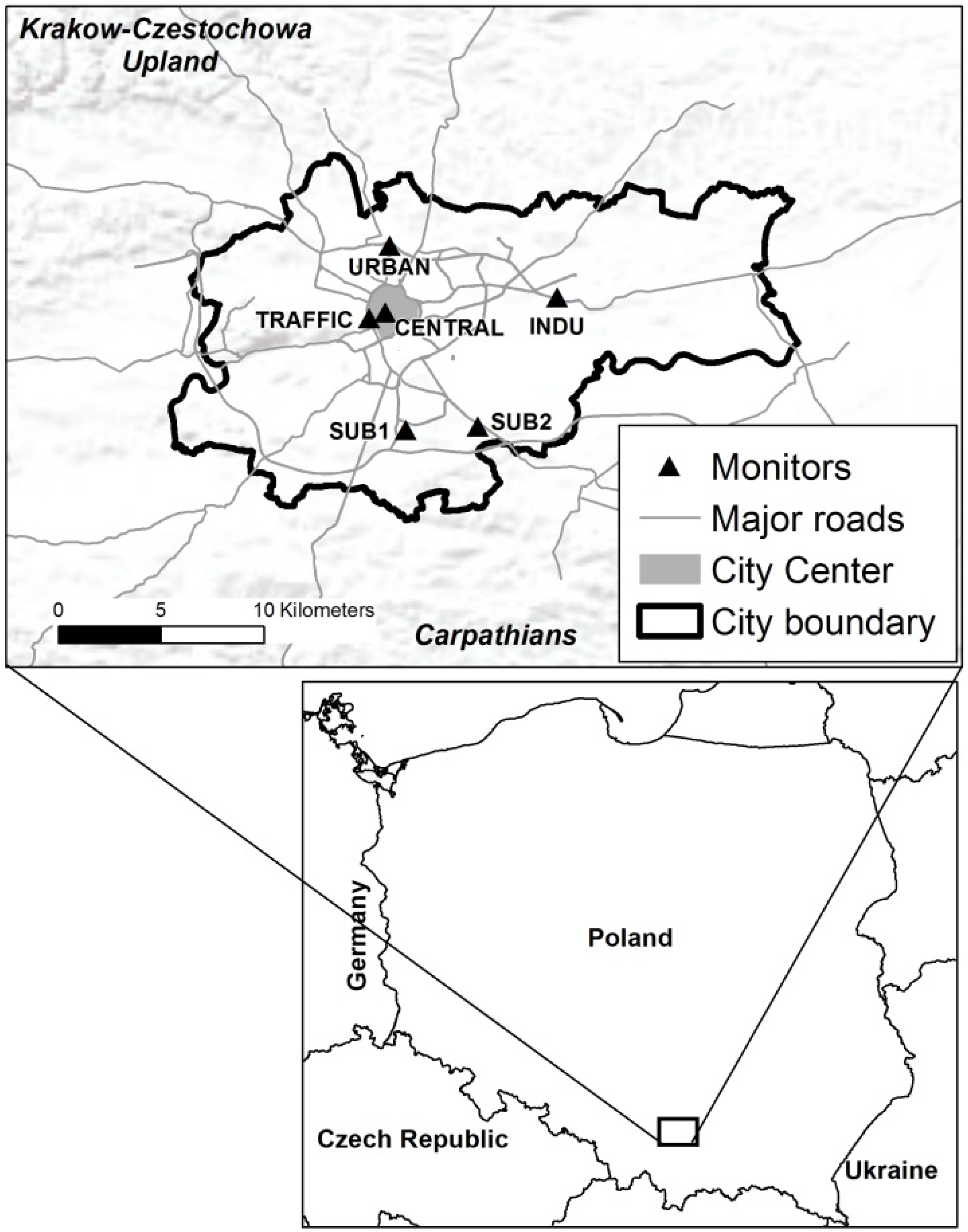
2.1. Study Site Characterization
2.2. The Air Pollutant Sampling and Analysis

2.3. Statistical Analysis
2.3.1. Descriptive Analysis
2.3.2. Linear Regression Model
2.3.3. Generalized Linear Mixed Effects Model
3. Results and Discussion
3.1. Descriptive Analyses
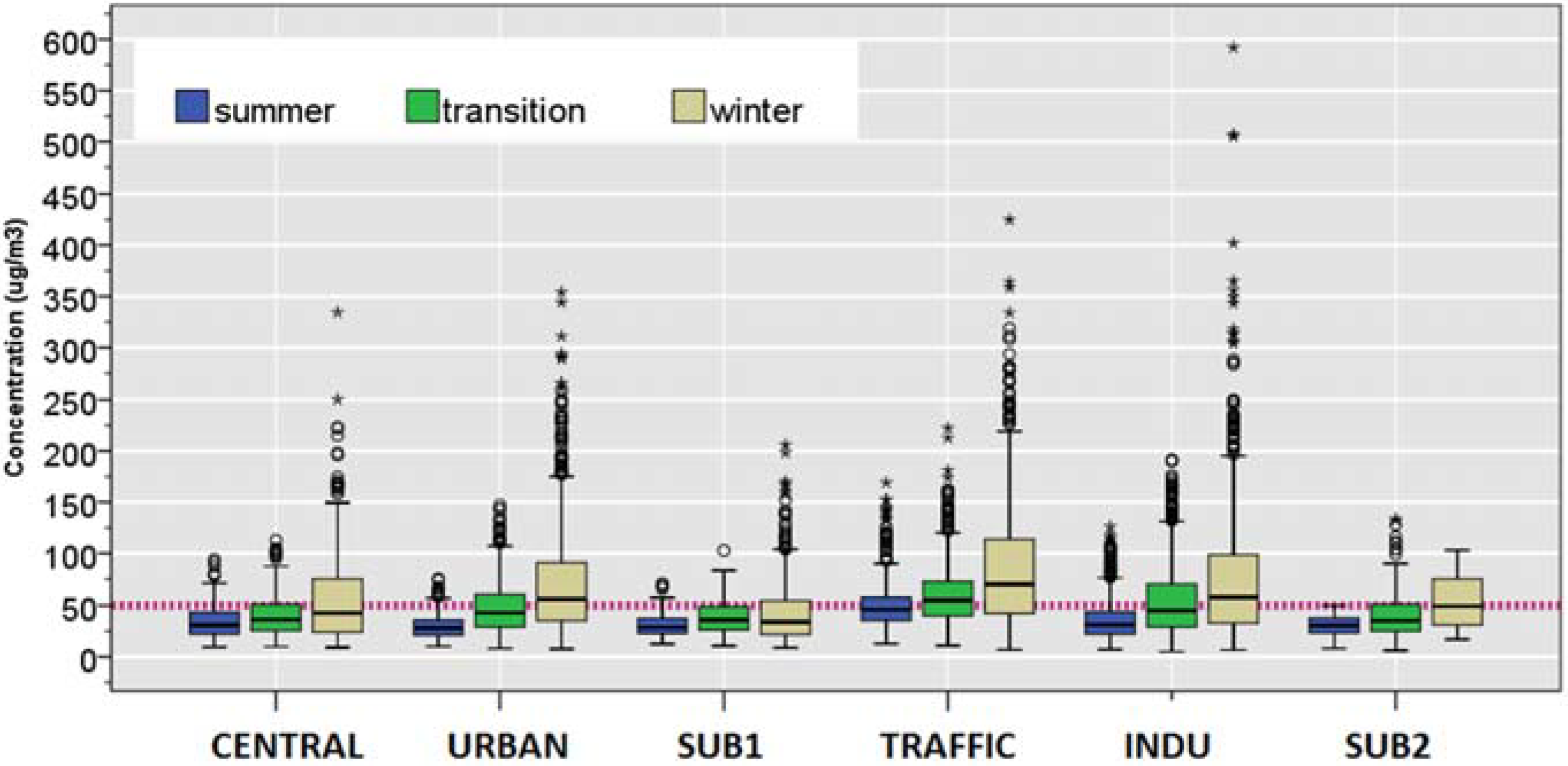
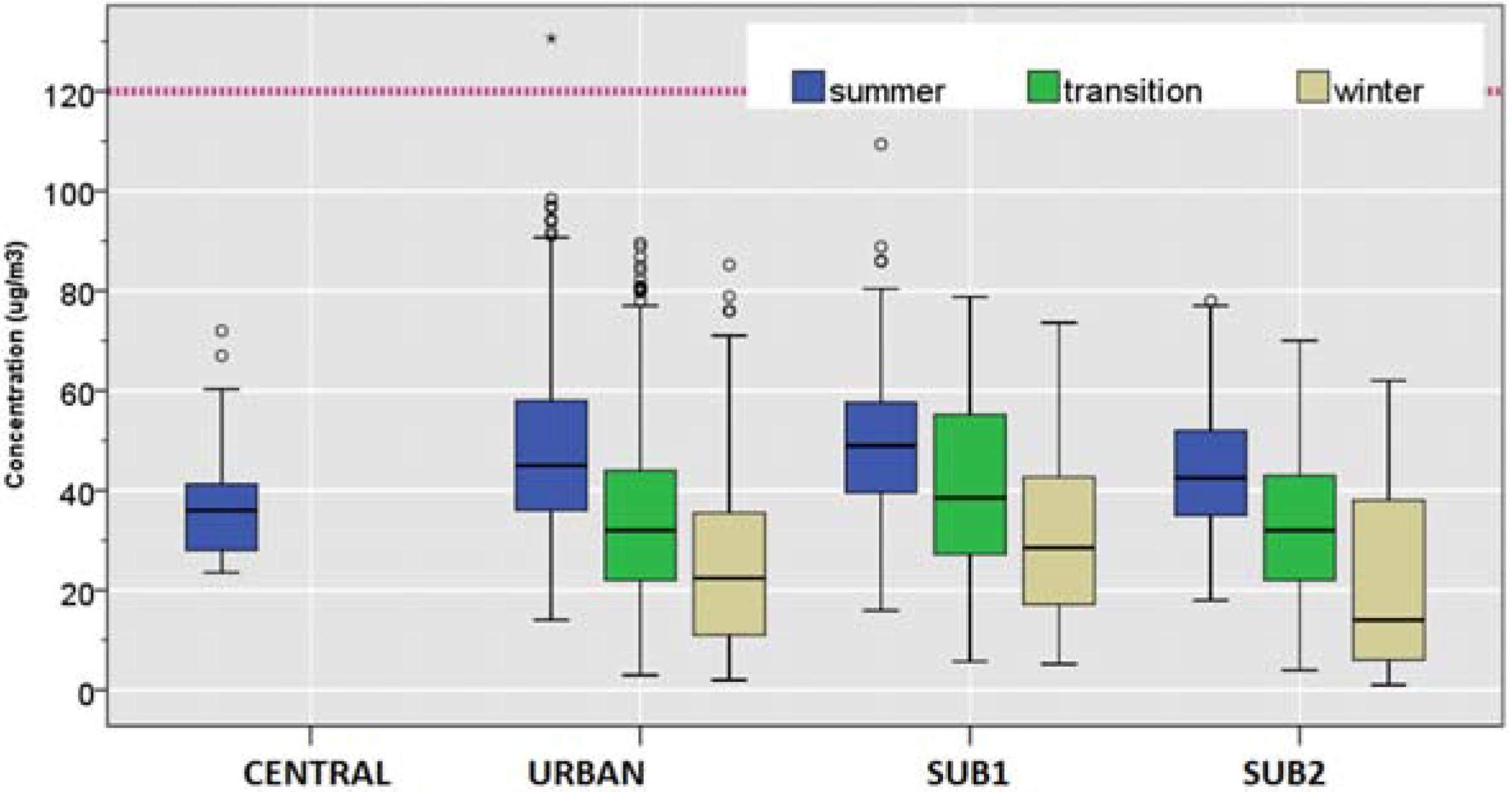
3.1.1. PM10

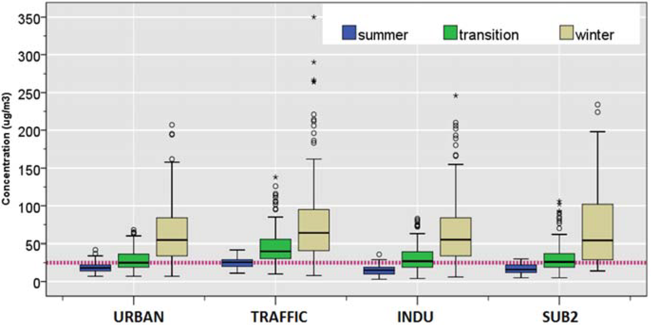
3.1.2. PM2.5
3.2. PM2.5 and PM10 Relationship
3.2.1. PM2.5/PM10 Concentration Ratio
3.2.2. Pearson’s Correlation Coefficients
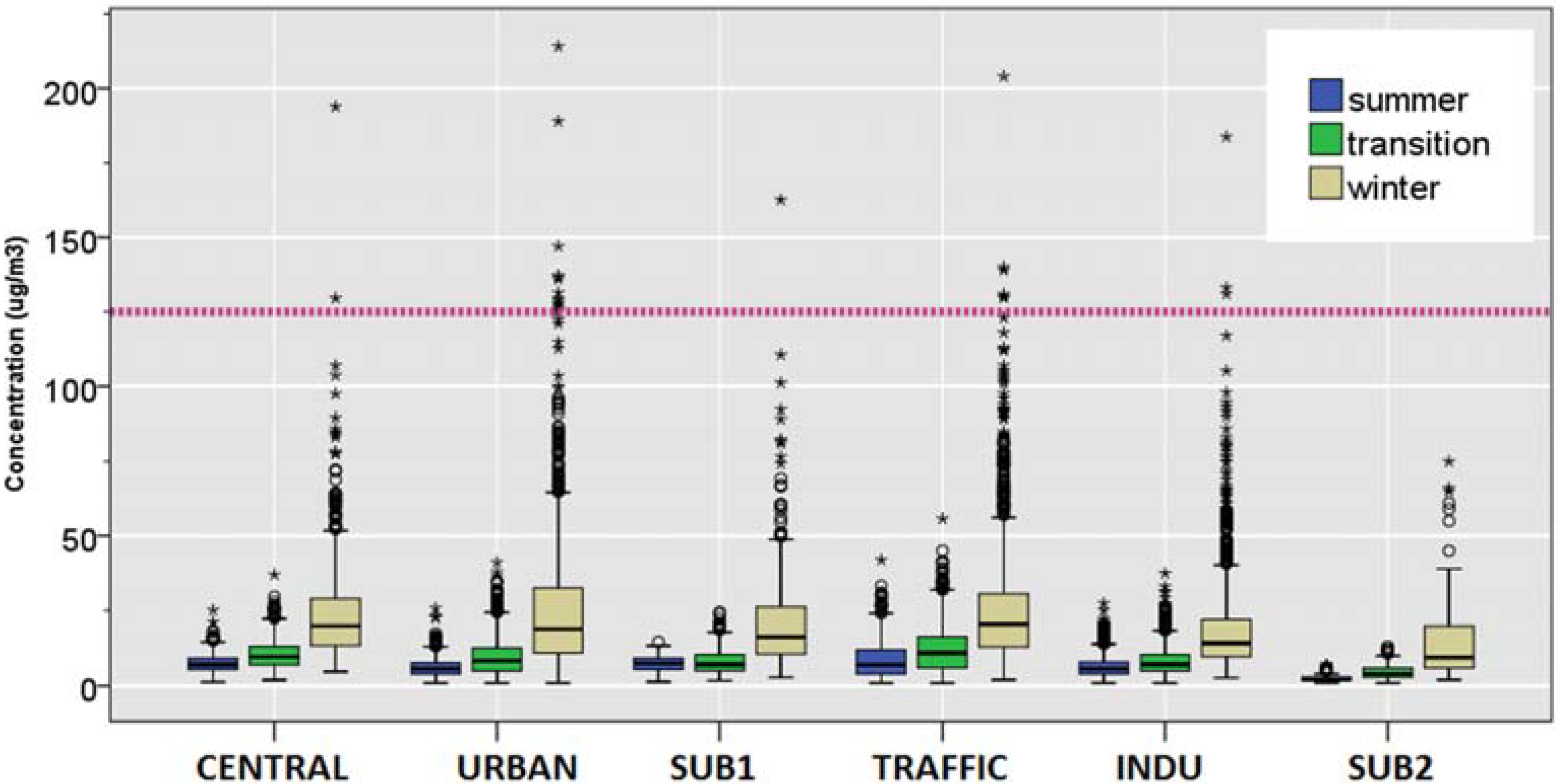
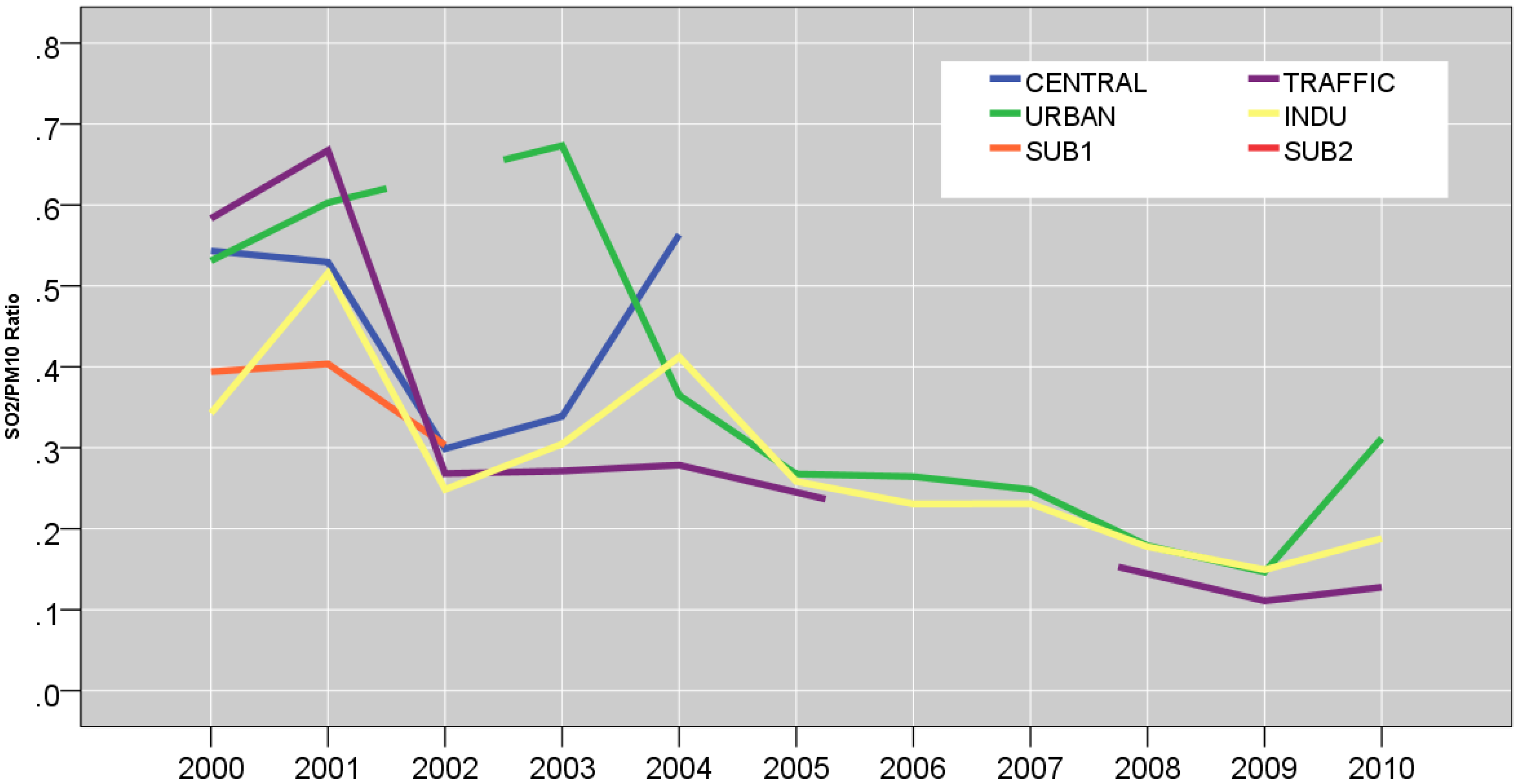
3.2.3. SO2

| PM2.5 (μg/m3) | PM10 (μg/m3) | PM2.5/PM10 | |||||||||
|---|---|---|---|---|---|---|---|---|---|---|---|
| N | Mean ± SD | Min | Max | >25 a (%) | N | Mean ± SD | Min | Max | >50 a (%) | Mean ± SD | |
| CENTRAL | |||||||||||
| summer | 305 | 33.7 ± 14.6 | 9.4 | 93.9 | 33(3%) | ||||||
| transition | 459 | 39.8 ± 18.8 | 9.8 | 112.6 | 123 (9%) | ||||||
| winter | 507 | 55.3 ± 43.0 | 9.2 | 334.3 | 210 (13%) | ||||||
| winter/summer | 1.4 | ||||||||||
| URBAN | |||||||||||
| summer | 90 | 18.7 ± 6.5 | 7.0 | 42.0 | 12 (1%) | 495 | 29.2 ± 11.0 | 10.0 | 75.0 | 18 (2%) | 0.7 ± 0.1 |
| transition | 120 | 28.8 ± 13.7 | 7.0 | 68.0 | 57 (4%) | 751 | 47.5 ± 24.3 | 8.0 | 147.0 | 281 (21%) | 0.6 ± 0.1 |
| winter | 202 | 62.8 ± 37.0 | 7.0 | 207.0 | 180 (11%) | 1069 | 69.5 ± 49.6 | 7.7 | 354.0 | 598 (36%) | 0.8 ± 0.1 |
| winter/summer | 3.0 | 2.0 | |||||||||
| TRAFFIC | |||||||||||
| summer | 116 | 25.2 ± 7.0 | 11.0 | 42.0 | 58 (6%) | 548 | 49.1 ± 22.8 | 12.8 | 169.1 | 214 (21%) | 0.6 ± 0.1 |
| transition | 132 | 46.1 ± 24.8 | 10.0 | 138.0 | 113 (8%) | 700 | 59.2 ± 29.4 | 11.0 | 222.4 | 414 (31%) | 0.7 ± 0.1 |
| winter | 209 | 76.6 ± 52.6 | 8.0 | 350.0 | 191 (12%) | 947 | 85.7 ± 58.9 | 6.8 | 424.8 | 644 (39%) | 0.7 ± 0.1 |
| winter/summer | 2.5 | 1.5 | |||||||||
| INDU | |||||||||||
| summer | 109 | 14.9 ± 6.6 | 3.0 | 36.0 | 7 (1%) | 890 | 35.8 ± 18.7 | 7.0 | 126.0 | 158 (16%) | 0.5 ± 0.1 |
| transition | 167 | 30.9 ± 16.3 | 4.0 | 83.0 | 90 (7%) | 1147 | 53.0 ± 32.1 | 5.0 | 191.0 | 502 (37%) | 0.6 ± 0.1 |
| winter | 242 | 65.4 ± 42.1 | 6.0 | 246.0 | 211 (13%) | 1491 | 73.2 ± 57.1 | 6.6 | 592.0 | 856 (51%) | 0.8 ± 0.1 |
| winter/summer | 3.7 | 1.9 | |||||||||
| SUB1 | |||||||||||
| summer | 202 | 31.4 ± 11.5 | 12.4 | 70.5 | 14 (1%) | ||||||
| transition | 297 | 38.6 ± 16.8 | 10.5 | 102.6 | 72 (5%) | ||||||
| winter | 385 | 44.8 ± 33.0 | 8.6 | 206.0 | 110 (7%) | ||||||
| winter/summer | 1.2 | ||||||||||
| SUB2 | |||||||||||
| summer | 89 | 16.8 ± 6.3 | 5.0 | 30.0 | 9 (1%) | 84 | 30.2 ± 10.0 | 8.0 | 50.0 | 0 (0%) | 0.6 ± 0.1 |
| transition | 118 | 31.6 ± 21.1 | 5.0 | 106.0 | 60 (5%) | 119 | 42.4 ± 26.8 | 6.0 | 133.0 | 30 (2%) | 0.7 ± 0.1 |
| winter | 61 | 71.8 ± 56.6 | 14.0 | 234.0 | 49 (3%) | 30 | 55.0 ± 27.1 | 17.0 | 103.0 | 14 (1%) | 0.8 ± 0.1 |
| winter/summer | 3.4 | 1.6 | |||||||||
| PM10 | PM2.5 | ||||||||||
|---|---|---|---|---|---|---|---|---|---|---|---|
| CENTRAL | URBAN | SUB1 | TRAFFIC | INDU | SUB2 | URBAN | TRAFFIC | INDU | SUB2 | ||
| PM10 | CENTRAL | 1 | 0.829 ** | 0.875 ** | 0.835 ** | 0.833 ** | |||||
| URBAN | 1 | 0.841 ** | 0.751 ** | 0.898 ** | 0.961 ** | 0.951 ** | 0.928 ** | ||||
| SUB1 | 1 | 0.737 ** | 0.825 ** | ||||||||
| TRAFFIC | 1 | 0.836 ** | 0.903 ** | 0.880 ** | 0.944 ** | 0.911 ** | 0.904 ** | ||||
| INDU | 1 | 0.888 ** | 0.886 ** | 0.918 ** | 0.963 ** | 0.896 ** | |||||
| SUB2 | 1 | 0.871 ** | 0.826 ** | 0.947 ** | |||||||
| PM2.5 | URBAN | 1 | 0.967 ** | 0.957 ** | |||||||
| TRAFFIC | 1 | 0.951 ** | 0.953 ** | ||||||||
| INDU | 1 | 0.947 ** | |||||||||
| SUB2 | 1 | ||||||||||
| Site Name | Predictor | β | (95% CI) | Adjusted-R2 |
|---|---|---|---|---|
| URBAN | y-intercept | −0.14 | (−0.32 0.05) | |
| (Ln) PM10 | 0.92 | (0.87 0.97) | 0.914 | |
| TRAFFIC | y-intercept | 0.62 | (−0.31 1.54) | |
| (Ln) PM10 | 0.74 | (0.51 0.97) | 0.602 | |
| INDU | y-intercept | −0.53 | (−0.65 −0.40) | |
| (Ln) PM10 | 1.00 | (0.97 1.03) | 0.931 | |
| SUB2 | y-intercept | −0.38 | (−0.57 −0.18) | |
| (Ln) PM10 | 0.99 | (0.94 1.04) | 0.909 |
| SO2 | O3 | NO2 | ||||||||||
|---|---|---|---|---|---|---|---|---|---|---|---|---|
| N | Mean ± SD | MIN | MAX | N | Mean ± SD | MIN | MAX | N | Mean ± SD | MIN | MAX | |
| CENTRAL | ||||||||||||
| summer | 360 | 7.7 ± 3.4 | 1.3 | 25.1 | 29 | 38.0 ± 12.8 | 23.5 | 72.0 | 246 | 23.6 ± 6.7 | 9.7 | 43.5 |
| transition | 545 | 10.6 ± 5.1 | 1.9 | 37.0 | 399 | 29.2 ± 9.4 | 8.9 | 60.1 | ||||
| winter | 672 | 24.2 ± 17.1 | 4.7 | 193.9 | 621 | 35.2 ± 13.1 | 11.3 | 93.6 | ||||
| winter/summer | 2.8 | 1.5 | ||||||||||
| URBAN | ||||||||||||
| summer | 711 | 6.1 ± 3.3 | 1.0 | 25.8 | 649 | 48.3 ± 16.7 | 14.0 | 130.6 | 611 | 29.7 ± 8.7 | 8.5 | 59.0 |
| transition | 1051 | 9.7 ± 6.2 | 1.0 | 41.1 | 872 | 33.8 ± 16.6 | 3.0 | 89.6 | 981 | 33.9 ± 10.7 | 8.6 | 68.5 |
| winter | 1397 | 25.3 ± 21.9 | 1.0 | 214.1 | 1131 | 24.5 ± 16.0 | 2.0 | 85.2 | 1192 | 37.7 ± 16.5 | 7.0 | 130.0 |
| winter/summer | 3.3 | 0.5 | 1.2 | |||||||||
| TRAFFIC | ||||||||||||
| summer | 915 | 8.6 ± 5.9 | 1.0 | 41.9 | 874 | 70.5 ± 15.5 | 25.7 | 125.7 | ||||
| transition | 1236 | 12.0 ± 7.7 | 1.0 | 55.8 | 1226 | 69.0 ± 16.4 | 21.7 | 123.5 | ||||
| winter | 1582 | 25.0 ± 19.2 | 2.0 | 204.1 | 1526 | 62.3 ± 19.3 | 20.8 | 152.6 | ||||
| winter/summer | 2.9 | 0.9 | ||||||||||
| INDU | ||||||||||||
| summer | 849 | 6.5 ± 3.7 | 1.0 | 27.3 | 884 | 25.0 ± 7.1 | 7.0 | 53.9 | ||||
| transition | 1116 | 8.3 ± 4.8 | 1.0 | 37.5 | 1152 | 28.7 ± 9.1 | 2.7 | 61.0 | ||||
| winter | 1509 | 18.3 ± 14.9 | 2.7 | 183.7 | 1586 | 35.2 ± 14.3 | 7.0 | 130.0 | ||||
| winter/summer | 2.5 | 1.3 | ||||||||||
| SUB1 | ||||||||||||
| summer | 182 | 7.6 ± 2.7 | 1.3 | 14.7 | 179 | 49.3 ± 13.9 | 15.9 | 109.4 | 169 | 25.1 ± 7.9 | 7.3 | 49.7 |
| transition | 266 | 8.2 ± 4.4 | 1.7 | 24.4 | 204 | 41.2 ± 17.4 | 5.7 | 78.8 | 261 | 28.8 ± 9.2 | 6.7 | 57.1 |
| winter | 350 | 21.6 ± 18.1 | 2.8 | 162.6 | 287 | 30.6 ± 15.9 | 5.2 | 73.6 | 302 | 32.6 ± 13.2 | 6.7 | 80.8 |
| winter/summer | 2.2 | 0.6 | 1.3 | |||||||||
| SUB2 | ||||||||||||
| summer | 87 | 2.7 ± 1.4 | 1.0 | 7.0 | 86 | 44.5 ± 14.1 | 18.0 | 78.0 | 86 | 31.5 ± 9.2 | 14.0 | 56.0 |
| transition | 120 | 4.8 ± 2.9 | 1.0 | 13.0 | 117 | 32.5 ± 14.7 | 4.0 | 70.0 | 112 | 31.3 ± 11.2 | 12.0 | 68.0 |
| winter | 58 | 17.6 ± 18.2 | 2.0 | 75.0 | 69 | 21.7 ± 19.0 | 1.0 | 62.0 | 69 | 40.2 ± 16.0 | 17.0 | 87.0 |
| winter/summer | 4.8 | 0.3 | 1.3 | |||||||||


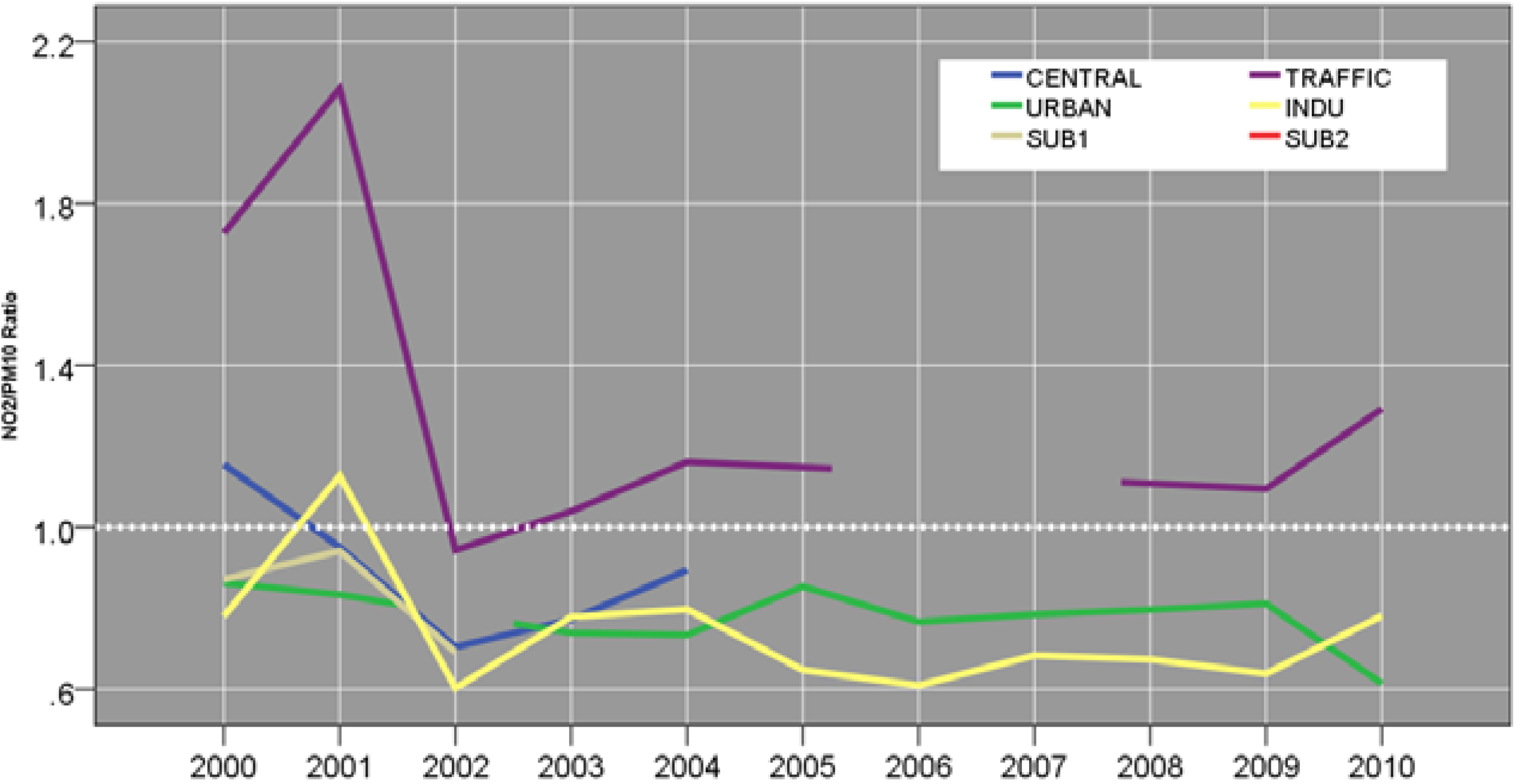
3.2.4. NO2


| Numerator | URBAN | TRAFFIC | INDU | SUB1 | ||||||
|---|---|---|---|---|---|---|---|---|---|---|
| Denominator | CENTRAL | CENTRAL | CENTRAL | CENTRAL | ||||||
| N | Mean ± SD | N | Mean ± SD | N | Mean ± SD | N | Mean ± SD | |||
| PM10 | Summer | 70 | 1.2 ± 0.4 | 279 | 1.5 ± 0.5 | 263 | 1.1 ± 0.4 | 161 | 1.2 ± 0.3 | |
| Transition | 152 | 1.3 ± 0.4 | 419 | 1.5 ± 0.5 | 420 | 1.3 ± 0.6 | 271 | 1.1 ± 0.3 | ||
| Winter | 135 | 1.3 ± 0.4 | 496 | 1.9 ± 0.7 | 483 | 1.3 ± 0.4 | 263 | 1.2 ± 0.4 | ||
| Overall | 357 | 1.3 ± 0.4 | 1194 | 1.7 ± 0.6 | 1166 | 1.3 ± 0.5 | 695 | 1.1 ± 0.3 | ||
| SO2 | Summer | 253 | 1.1 ± 0.5 | 321 | 1.8 ± 0.6 | 281 | 1.1 ± 0.5 | 132 | 1.1 ± 0.4 | |
| Transition | 464 | 1.2 ± 0.5 | 522 | 1.8 ± 0.6 | 411 | 0.9 ± 0.4 | 265 | 0.8 ± 0.5 | ||
| Winter | 604 | 1.3 ± 0.4 | 650 | 1.3 ± 0.3 | 575 | 0.9 ± 0.3 | 333 | 0.9 ± 0.3 | ||
| Overall | 1321 | 1.2 ± 0.4 | 1493 | 1.6 ± 0.6 | 1267 | 0.9 ± 0.4 | 730 | 0.9 ± 0.4 | ||
| NO2 | Summer | 92 | 1.3 ± 0.3 | 197 | 3.3 ± 0.7 | 213 | 1.2 ± 0.3 | 128 | 1.1 ± 0.2 | |
| Transition | 262 | 1.1 ± 0.3 | 376 | 2.5 ± 0.7 | 297 | 1.1 ± 0.3 | 200 | 1.0 ± 0.2 | ||
| Winter | 347 | 1.1 ± 0.3 | 584 | 1.8 ± 0.4 | 580 | 1.0 ± 0.2 | 269 | 1.0 ± 0.3 | ||
| Overall | 701 | 1.1 ± 0.3 | 1157 | 2.3 ± 0.8 | 1090 | 1.0 ± 0.2 | 597 | 1.0 ± 0.3 | ||
3.2.5. O3
3.3. Regression Model Results

3.3.1. Site Effect
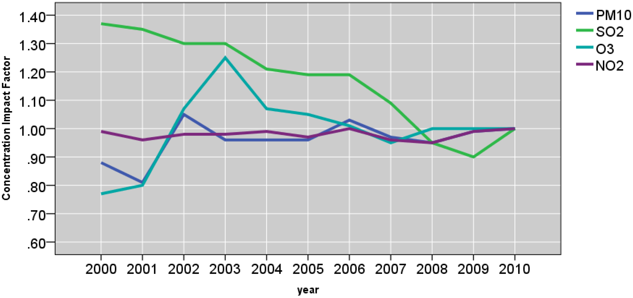
3.3.2. Year Effect
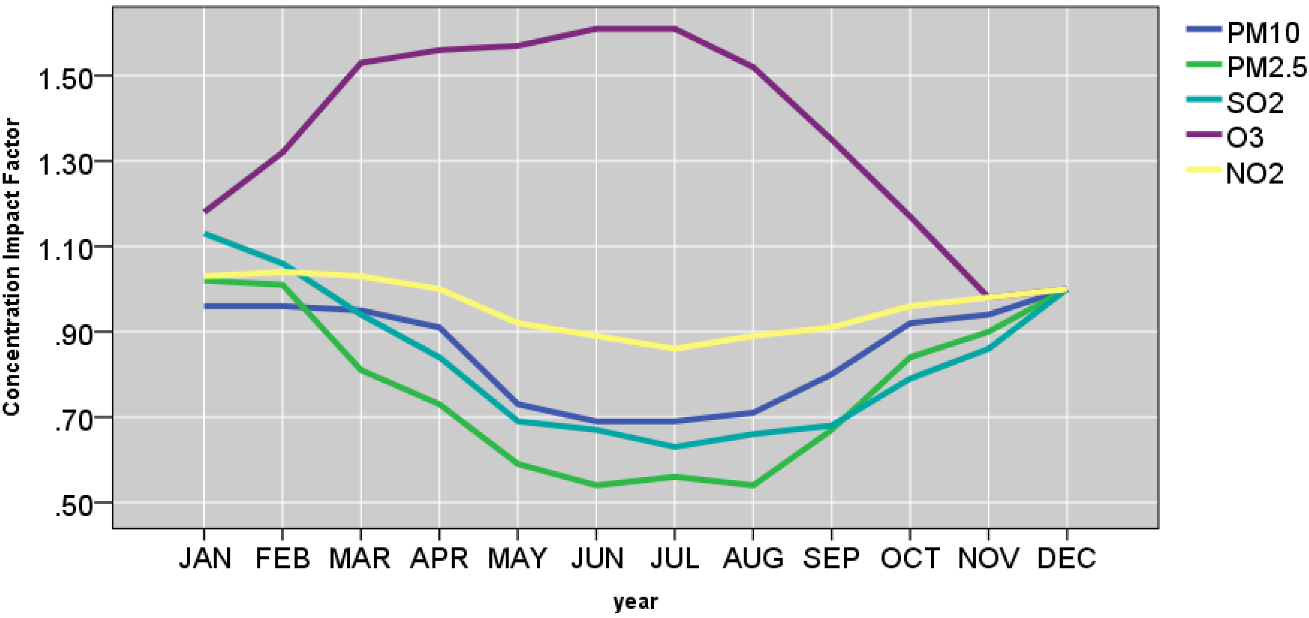
3.3.3. Month Effect
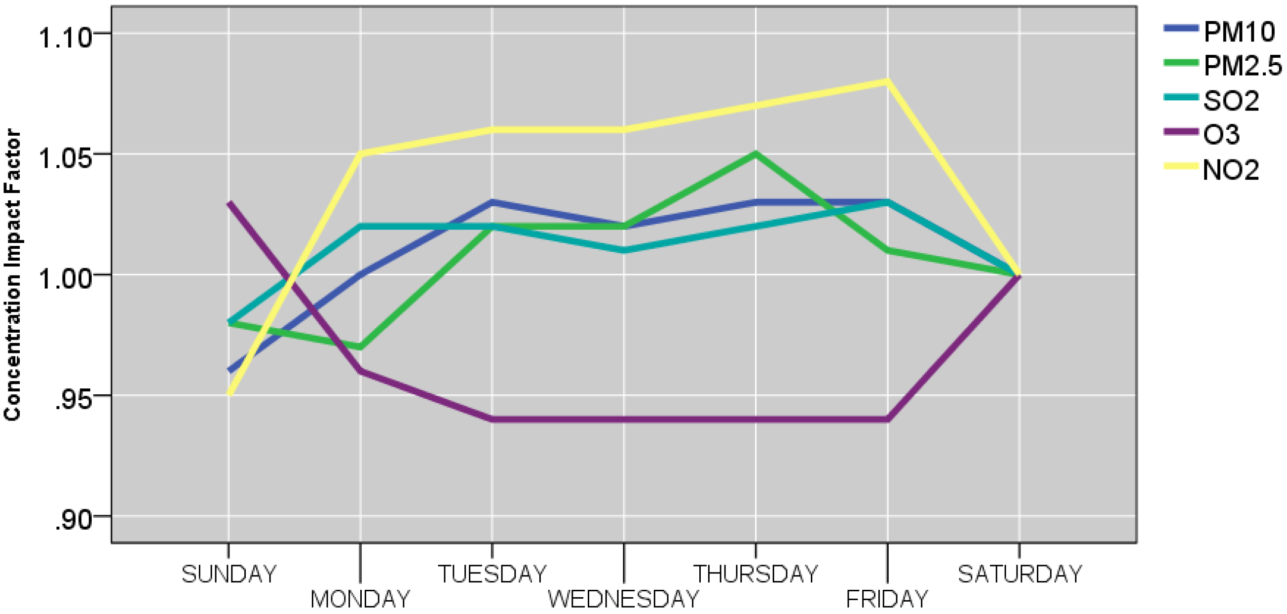
3.3.4. Weekday Effect
4. Conclusions
Acknowledgments
Author Contributions
Appendix
| Predictors | PM10 | PM2.5 | SO2 | NO2 | O3 | |||||||||||
|---|---|---|---|---|---|---|---|---|---|---|---|---|---|---|---|---|
| β | SE | IF | β | SE | IF | β | SE | IF | β | SE | IF | β | SE | IF | ||
| Intercept | 1.7 | 0.0 | 5.6 | 1.7 | 0.0 | 5.4 | 0.9 | 0.0 | 2.6 | 1.5 | 0.0 | 4.3 | 1.2 | 0.1 | 3.2 | |
| Year | 2000 | −0.1 | 0.0 | 0.9 | 0.3 | 0.0 | 1.4 | 0.0 | 0.0 | 1.0 | −0.3 | 0.1 | 0.8 | |||
| 2001 | −0.2 | 0.0 | 0.8 | 0.3 | 0.0 | 1.4 | 0.0 | 0.0 | 1.0 | −0.2 | 0.1 | 0.8 | ||||
| 2002 | 0.1 | 0.0 | 1.1 | 0.3 | 0.0 | 1.3 | 0.0 | 0.0 | 1.0 | 0.1 | 0.0 | 1.1 | ||||
| 2003 | 0.0 | 0.0 | 1.0 | 0.3 | 0.0 | 1.3 | 0.0 | 0.0 | 1.0 | 0.2 | 0.0 | 1.3 | ||||
| 2004 | 0.0 | 0.0 | 1.0 | 0.2 | 0.0 | 1.2 | 0.0 | 0.0 | 1.0 | 0.1 | 0.0 | 1.1 | ||||
| 2005 | 0.0 | 0.0 | 1.0 | 0.2 | 0.0 | 1.2 | 0.0 | 0.0 | 1.0 | 0.1 | 0.0 | 1.1 | ||||
| 2006 | 0.0 | 0.0 | 1.0 | 0.2 | 0.0 | 1.2 | 0.0 | 0.0 | 1.0 | 0.0 | 0.0 | 1.0 | ||||
| 2007 | 0.0 | 0.0 | 1.0 | 0.1 | 0.0 | 1.1 | 0.0 | 0.0 | 1.0 | −0.1 | 0.0 | 1.0 | ||||
| 2008 | −0.1 | 0.0 | 1.0 | −0.1 | 0.0 | 1.0 | −0.1 | 0.0 | 1.0 | 0.0 | 0.0 | 1.0 | ||||
| 2009 | 0.0 | 0.0 | 1.0 | 0.0 | 0.0 | 1.0 | −0.1 | 0.0 | 0.9 | 0.0 | 0.0 | 1.0 | 0.0 | 0.0 | 1.0 | |
| 2010 | 0.0 | 1.0 | 0.0 | 1.0 | 0.0 | 1.0 | 0.0 | 1.0 | 0.0 | 1.0 | ||||||
| Month | January | 0.0 | 0.0 | 1.0 | 0.0 | 0.0 | 1.0 | 0.1 | 0.0 | 1.1 | 0.0 | 0.0 | 1.0 | 0.2 | 0.0 | 1.2 |
| February | 0.0 | 0.0 | 1.0 | 0.0 | 0.0 | 1.0 | 0.1 | 0.0 | 1.1 | 0.0 | 0.0 | 1.0 | 0.3 | 0.0 | 1.3 | |
| March | −0.1 | 0.0 | 1.0 | −0.2 | 0.0 | 0.8 | −0.1 | 0.0 | 0.9 | 0.0 | 0.0 | 1.0 | 0.4 | 0.0 | 1.5 | |
| April | −0.1 | 0.0 | 0.9 | −0.3 | 0.0 | 0.7 | −0.2 | 0.0 | 0.8 | 0.0 | 0.0 | 1.0 | 0.5 | 0.0 | 1.6 | |
| May | −0.3 | 0.0 | 0.7 | −0.5 | 0.0 | 0.6 | −0.4 | 0.0 | 0.7 | −0.1 | 0.0 | 0.9 | 0.5 | 0.0 | 1.6 | |
| June | −0.4 | 0.0 | 0.7 | −0.6 | 0.0 | 0.5 | −0.4 | 0.0 | 0.7 | −0.1 | 0.0 | 0.9 | 0.5 | 0.0 | 1.6 | |
| July | −0.4 | 0.0 | 0.7 | −0.6 | 0.1 | 0.6 | −0.5 | 0.0 | 0.6 | −0.2 | 0.0 | 0.9 | 0.5 | 0.0 | 1.6 | |
| August | −0.3 | 0.0 | 0.7 | −0.6 | 0.0 | 0.5 | −0.4 | 0.0 | 0.7 | −0.1 | 0.0 | 0.9 | 0.4 | 0.0 | 1.5 | |
| September | −0.2 | 0.0 | 0.8 | −0.4 | 0.0 | 0.7 | −0.4 | 0.0 | 0.7 | −0.1 | 0.0 | 0.9 | 0.3 | 0.0 | 1.4 | |
| October | −0.1 | 0.0 | 0.9 | −0.2 | 0.0 | 0.8 | −0.2 | 0.0 | 0.8 | 0.0 | 0.0 | 1.0 | 0.2 | 0.0 | 1.2 | |
| November | −0.1 | 0.0 | 0.9 | −0.1 | 0.0 | 0.9 | −0.2 | 0.0 | 0.9 | 0.0 | 0.0 | 1.0 | 0.0 | 0.0 | 1.0 | |
| December | 0.0 | 1.0 | 0.0 | 1.0 | 0.0 | 1.0 | 0.0 | 1.0 | 0.0 | 1.0 | ||||||
| Day | Sunday | 0.0 | 0.0 | 1.0 | 0.0 | 0.0 | 1.0 | 0.0 | 0.0 | 1.0 | −0.1 | 0.0 | 1.0 | 0.0 | 0.0 | 1.0 |
| Monday | 0.0 | 0.0 | 1.0 | 0.0 | 0.0 | 1.0 | 0.0 | 0.0 | 1.0 | 0.1 | 0.0 | 1.1 | 0.0 | 0.0 | 1.0 | |
| Tuesday | 0.0 | 0.0 | 1.0 | 0.0 | 0.0 | 1.0 | 0.0 | 0.0 | 1.0 | 0.1 | 0.0 | 1.1 | −0.1 | 0.0 | 0.9 | |
| Wednesday | 0.0 | 0.0 | 1.0 | 0.0 | 0.0 | 1.0 | 0.0 | 0.0 | 1.0 | 0.1 | 0.0 | 1.1 | −0.1 | 0.0 | 0.9 | |
| Thursday | 0.0 | 0.0 | 1.0 | 0.1 | 0.0 | 1.1 | 0.0 | 0.0 | 1.0 | 0.1 | 0.0 | 1.1 | −0.1 | 0.0 | 0.9 | |
| Friday | 0.0 | 0.0 | 1.0 | 0.0 | 0.0 | 1.0 | 0.0 | 0.0 | 1.0 | 0.1 | 0.0 | 1.1 | −0.1 | 0.0 | 0.9 | |
| Saturday | 0.0 | 1.0 | 0.0 | 1.0 | 0.0 | 1.0 | 0.0 | 1.0 | 0.0 | 1.0 | ||||||
| Site | URBAN | 0.0 | 0.0 | 1.0 | 0.0 | 0.0 | 1.0 | 0.1 | 0.0 | 1.1 | 0.0 | 0.0 | 1.0 | 0.1 | 0.0 | 1.1 |
| SUB1 | 0.0 | 0.0 | 1.0 | −0.1 | 0.0 | 0.9 | 0.0 | 0.0 | 1.0 | 0.5 | 0.1 | 1.7 | ||||
| TRAFFIC | 0.2 | 0.0 | 1.2 | 0.1 | 0.0 | 1.1 | 0.1 | 0.0 | 1.1 | 0.4 | 0.0 | 1.4 | ||||
| INDU | 0.1 | 0.0 | 1.1 | 0.0 | 0.0 | 1.0 | 0.0 | 0.0 | 1.0 | 0.0 | 0.0 | 1.0 | ||||
| SUB2 | −0.1 | 0.0 | 1.0 | −0.1 | 0.0 | 0.9 | 0.0 | 0.0 | 1.0 | 0.1 | 0.1 | 1.1 | ||||
| CENTRAL | 0.0 | 1.0 | 0.0 | 1.0 | 0.0 | 1.0 | 0.0 | 1.0 | 0.0 | 1.0 | ||||||
| Temperature | < 4.9 | −0.1 | 0.0 | 1.0 | 0.0 | 0.0 | 1.0 | 0.1 | 0.0 | 1.1 | −0.1 | 0.0 | 0.9 | −0.1 | 0.0 | 0.9 |
| (°C) | 4.9−14.6 | −0.1 | 0.0 | 0.9 | 0.0 | 0.0 | 1.0 | 0.0 | 0.0 | 1.0 | −0.1 | 0.0 | 1.0 | -0.1 | 0.0 | 0.9 |
| ≥ 14.6 | 0.0 | 1.0 | 0.0 | 1.0 | 0.0 | 1.0 | 0.0 | 1.0 | 0.0 | 1.0 | ||||||
| Wind speed | < 0.90 | 0.2 | 0.0 | 1.2 | 0.2 | 0.0 | 1.3 | 0.1 | 0.0 | 1.1 | 0.1 | 0.0 | 1.1 | −0.1 | 0.0 | 0.9 |
| (m/sec) | ≥ 0.90 | 0.0 | 1.0 | 0.0 | 1.0 | 0.0 | 1.0 | 0.0 | 1.0 | 0.0 | 1.0 | |||||
Conflicts of Interest
References
- Worldwide Trends in the Prevalence of Asthma Symptoms: Phase III of the International Study of Asthma and Allergies in Childhood (ISAAC). Available online: http://thorax.bmj.com/content/62/9/758 (accessed on 5 January 2015).
- The Global Asthma Report 2011. Available online: http://www.globalasthmareport.org/2011/ (accessed on 5 January 2015).
- Bokwa, A. Environmental impacts of long-term air pollution changes in Krakow, Poland. Pol. J. Environ. Stud. 2008, 17, 673–686. [Google Scholar]
- Junninen, H.; Mønster, J.; Rey, M.; Cancelinha, J.; Douglas, K.; Duane, M.; Forcina, V.; Müller, A.; Lagler, F.; Marelli, L.; et al. Quantifying the impact of residential heating on the urban air quality in a typical european coal combustion region. Environ. Sci. Technol. 2009, 43, 7964–7970. [Google Scholar] [CrossRef] [PubMed]
- Lvovsky, K.; Hughes, G.; Maddison, D.; Ostro, B.; Pearce, D. Environmental Costs of Fossil Fuels: A Rapid Assessment Method with Application to Six Cities; 78; The World Bank Environment Department: Washington, DC, USA, 2000; p. 104. [Google Scholar]
- Nowicki, M. Environment in Poland. Issues and Solutions; Kluwer Academic Publishers: Dordrecht, The Ntherlands, 1993. [Google Scholar]
- Anderson, K. The political economy of coal subsidies in Europe. Energy Policy 1995, 23, 485–496. [Google Scholar] [CrossRef]
- Zmirou, D.; Schwartz, J.; Saez, M.; Zanobett, A.; Wojtyniak, B.; Touloumi, G.; Spix, C.; de León, A.P.; Le Moullec, Y.; Bacharova, L. Time-series analysis of air pollution and cause specific mortality. Epidemiology 1998, 9, 495–503. [Google Scholar] [CrossRef] [PubMed]
- Bobak, M.; Feachem, R.G. Air pollution and mortality in Central and Eastern Europe An estimate of the impact. Eur J. Public Health 1995, 5, 82–86. [Google Scholar] [CrossRef]
- Jedrychowski, W.; Bendkowska, I.; Flak, E.; Penar, A.; Jacek, R.; Kaim, I.; Spengler, J.D.; Camann, D.; Perera, F.P. Estimated risk for altered fetal growth resulting from exposure to fine particles during pregnancy: An epidemiologic prospective cohort study in Poland. Environ. Health Perspect. 2004, 112, 1398–1402. [Google Scholar] [CrossRef] [PubMed]
- Jedrychowski, W.; Maugeri, U.; Perera, F.P.; Mroz, E.; Klimaszewska-Rembiasz, M.; Flak, E.; Edwards, S.; Majewska, R.; Sowa, A. Early wheeze as reported by mothers and lung function in 4-year-olds. Prospective cohort study in Krakow. Pediatr. Pulmonol. 2010, 45, 919–926. [Google Scholar] [CrossRef] [PubMed]
- Jedrychowski, W.; Perera, F.P.; Maugeri, U.; Mrozek-Budzyn, D.; Mroz, E.; Flak, E.; Edwards, S.; Spengler, J.D.; Jacek, R.; Sowa, A.; et al. Early wheezing phenotypes and severity of respiratory illness in very early childhood: Study on intrauterine exposure to fine particle matter. Environ. Inter. 2009, 35, 877–884. [Google Scholar] [CrossRef]
- Jedrychowski, W.A.; Perera, F.P.; Majewska, R.; Camman, D.; Spengler, J.D.; Mroz, E.; Stigter, L.; Flak, E.; Jacek, R. Separate and joint effects of tranplacental and postnatal inhalatory exposure to polycyclic aromatic hydrocarbons: Prospective birth cohort study on wheezing events. Pediatr. Pulmonol. 2014, 49, 162–172. [Google Scholar] [CrossRef] [PubMed]
- Jedrychowski, W.A.; Perera, F.P.; Maugeri, U.; Majewska, R.; Mroz, E.; Flak, E.; Camann, D.; Sowa, A.; Jacek, R. Long term effects of prenatal and postnatal airborne PAH exposures on ventilatory lung function of non-asthmatic preadolescent children. Prospective birth cohort study in Krakow. Sci. Total Environ 2015, 502, 502–509. [Google Scholar] [CrossRef] [PubMed]
- Jedrychowski, W.A.; Perera, F.P.; Maugeri, U.; Mroz, E.; Klimaszewska-Rembiasz, M.; Flak, E.; Edwards, S.; Spengler, J.D. Effect of prenatal exposure to fine particulate matter on ventilatory lung function of preschool children of non-smoking mothers. Paediatr. Perinat. Epidemiol. 2010, 24, 492–501. [Google Scholar] [CrossRef] [PubMed]
- Sram, R.; Binkova, B.; Dejmek, J.; Bobak, M. Ambient air pollution and pregnancy outcomes: A review of the literature. Environ. Health Perspect. 2005, 113, 375–382. [Google Scholar] [CrossRef] [PubMed]
- Ritz, B.; Wilhelm, M. Ambient air pollution and adverse birth outcomes: Methodologic issues in an emerging field. Basic Clin. Pharmacol. Toxicol. 2008, 102, 182–190. [Google Scholar] [CrossRef] [PubMed]
- Li, N.; Hao, M.; Phalen, R.; Hinds, W.; Nel, A. Particulate air pollutants and asthma. A paradigm for the role of oxidative stress in PM-induced adverse health effects. Clin. Immunol. 2003, 109, 250–265. [Google Scholar] [CrossRef] [PubMed]
- Wilczyńska-Michalik, W. Air pollution and damage to the cultural heritage in cities—The decay of the cultural heritage of Kraków, [w:] Sustainable Urban Patterns around the Baltic Sea. Case Studies, vol. IV. Reports from the superbs project, urban. Environ. Manage. 2003, 2003, 42–53. [Google Scholar]
- Szafraniec, K.; Jedrychowski, W. Spatial variability and trends in ambient air concentrations of metals in Cracow, Poland. Int. J. Occup. Med. Environ. Health 2001, 14, 261–265. [Google Scholar] [PubMed]
- Choi, H.; Perera, F.; Pac, A.; Wang, L.; Flak, E.; Mroz, E.; Jacek, R.; Chai-Onn, T.; Jedrychowski, W.; Masters, E.; et al. Estimating individual-level exposure to airborne polycyclic aromatic hydrocarbons throughout the gestational period based on personal, indoor, and outdoor monitoring. Environ. Health Perspect. 2008, 116, 1509–1518. [Google Scholar] [CrossRef] [PubMed]
- Choi, H.; Spengler, J. Source attribution of personal exposure to airborne polycyclic aromatic hydrocarbon mixture using concurrent personal, indoor, and outdoor measurements. Environ. Int. 2014, 63, 173–181. [Google Scholar] [CrossRef] [PubMed]
- Choi, H.; Wang, L.; Lin, X.; Spengler, J.D.; Perera, F.P. Fetal window of vulnerability to airborne polycyclic aromatic hydrocarbons on proportional intrauterine growth restriction. PLoS One 2012, 7. [Google Scholar] [CrossRef]
- Jedrychowski, W.A.; Perera, F.P.; Pac, A.; Jacek, R.; Whyatt, R.M.; Spengler, J.D.; Dumyahn, T.S.; Sochacka-Tatara, E. Variability of total exposure to PM2.5 related to indoor and outdoor pollution sources Krakow study in pregnant women. Sci Total Environ. 2006, 366, 47–54. [Google Scholar] [CrossRef] [PubMed]
- Jedrychowski, W.A.; Perera, F.P.; Spengler, J.D.; Mroz, E.; Stigter, L.; Flak, E.; Majewska, R.; Klimaszewska-Rembiasz, M.; Jacek, R. Intrauterine exposure to fine particulate matter as a risk factor for increased susceptibility to acute broncho-pulmonary infections in early childhood. Int. J. Hyg. Environ. Health 2013, 216, 395–401. [Google Scholar] [CrossRef] [PubMed]
- Choi, H.; Jedrychowski, W.; Spengler, J.; Camann, D.E.; Whyatt, R.M.; Rauh, V.; Tsai, W.Y.; Perera, F.P. International studies of prenatal exposure to polycyclic aromatic hydrocarbons and fetal growth. Environ. Health Perspect. 2006, 114, 1744–1750. [Google Scholar] [PubMed]
- Jedrychowski, W.; Pac, A.; Choi, H.; Jacek, R.; Sochacka-Tatara, E.; Dumyahn, T.; Spengler, J.; Camman, D.; Perera, F.P. Personal exposure to fine particles and benzo[a]pyrene. Relation with indoor and outdoor concentrations of these pollutants in Krakow. Int. J. Occup. Med. Environ. Health 2007, 20, 339–348. [Google Scholar] [PubMed]
- Choi, H.; Perera, F.P. Sources of greater fetal vulnerability to airborne polycyclic aromatic hydrocarbons among African Americans. J. Epidemiol. Community Health 2010, 66, 121–126. [Google Scholar] [CrossRef] [PubMed]
- Choi, H.; Rauh, V.; Garfinkel, R.; Tu, Y.; Perera, F.P. Prenatal exposure to airborne polycyclic aromatic hydrocarbons and risk of intrauterine growth restriction. Environ. Health Perspect. 2008, 116, 658–665. [Google Scholar] [CrossRef] [PubMed]
- Kobus, D.; Iwanek, J.; Mitosek, G.; Mill, W. Global and Regional Earth-System Monitoring Using Satellite and in-situ Data (GEMS): Organization of Air Quality Monitoring Data Collection in Poland Review of Available Air Quality Data; Institute of Environmental Protection: Warsaw, Poland, 2007. [Google Scholar]
- Suh, H.H.; Spengler, J.D.; Koutrakis, P. Personal exposures to acid aerosols and ammonia. Environ. Sci. Technol. 1992, 26, 2507–2517. [Google Scholar] [CrossRef]
- Koutrakis, P.; Sax, S.N.; Sarnat, J.A.; Coull, B.; Demokritou, P.; Demokritou, P.; Oyola, P.; Garcia, J.; Gramsch, E. Analysis of PM10, PM2.5, and PM2.5–10 concentrations in Santiago, Chile, from 1989 to 2001. J. Air Waste Manage. Assoc. 2005, 55, 342–351. [Google Scholar] [CrossRef]
- Querol, X.; Alastuey, A.; Ruiz, C.R.; Artiñano, B.; Hansson, H.C.; Harrison, R.M.; Buringh, E.; ten Brink, H.M.; Lutz, M.; Bruckmann, P.; et al. Speciation and origin of PM10 and PM2.5 in selected European cities. Atmos. Environ. 2004, 38, 6547–6555. [Google Scholar] [CrossRef]
- WHO. WHO Air Quality Guidelines for Particulate Matter, Ozone, Nitrogen Dioxide and Sulfur Dioxide: Summary of Risk Assessment; WHO: Geneva, Switzerland, 2005. [Google Scholar]
- Suh, H.H.; Bahadori, T.; Vallarino, J.; Spengler, J.D. Criteria Air Pollutants and Toxic Air Pollutants. Available online: http://www.ncbi.nlm.nih.gov/pmc/articles/PMC1637676/ (accessed on 6 January 2015).
- Brozek, M.; Zejda, J.E.; Kowalska, M.; Gebus, M.; Kepa, K.; Igielski, M. Opposite trends of allergic disorders and respiratory symptoms in children over a period of large-scale ambient air pollution decline. Pol. J. Environ. Stud. 2010, 19, 1133–1138. [Google Scholar]
- Maliszewska-Kordybach, B.; Smreczak, B.; Klimkowicz-Pawlas, A. Concentrations, sources, and spatial distribution of individual polycyclic aromatic hydrocarbons (PAHs) in agricultural soils in the Eastern part of the EU: Poland as a case study. Sci. Total Environ. 2009, 407, 3746–3753. [Google Scholar] [CrossRef] [PubMed]
- Wróbel, A.; Rokita, E.; Maenhaut, W. Transport of traffic-related aerosols in urban areas. Sci. Total Environ. 2000, 257, 199–211. [Google Scholar] [CrossRef] [PubMed]
© 2015 by the authors; licensee MDPI, Basel, Switzerland. This article is an open access article distributed under the terms and conditions of the Creative Commons Attribution license (http://creativecommons.org/licenses/by/4.0/).
Share and Cite
Choi, H.; Melly, S.; Spengler, J. Intraurban and Longitudinal Variability of Classical Pollutants in Kraków, Poland, 2000–2010. Int. J. Environ. Res. Public Health 2015, 12, 4967-4991. https://doi.org/10.3390/ijerph120504967
Choi H, Melly S, Spengler J. Intraurban and Longitudinal Variability of Classical Pollutants in Kraków, Poland, 2000–2010. International Journal of Environmental Research and Public Health. 2015; 12(5):4967-4991. https://doi.org/10.3390/ijerph120504967
Chicago/Turabian StyleChoi, Hyunok, Steven Melly, and John Spengler. 2015. "Intraurban and Longitudinal Variability of Classical Pollutants in Kraków, Poland, 2000–2010" International Journal of Environmental Research and Public Health 12, no. 5: 4967-4991. https://doi.org/10.3390/ijerph120504967