
A Spatial Framework to Map Heat Health Risks at Multiple Scales


Abstract
:1. Introduction
2. Methods
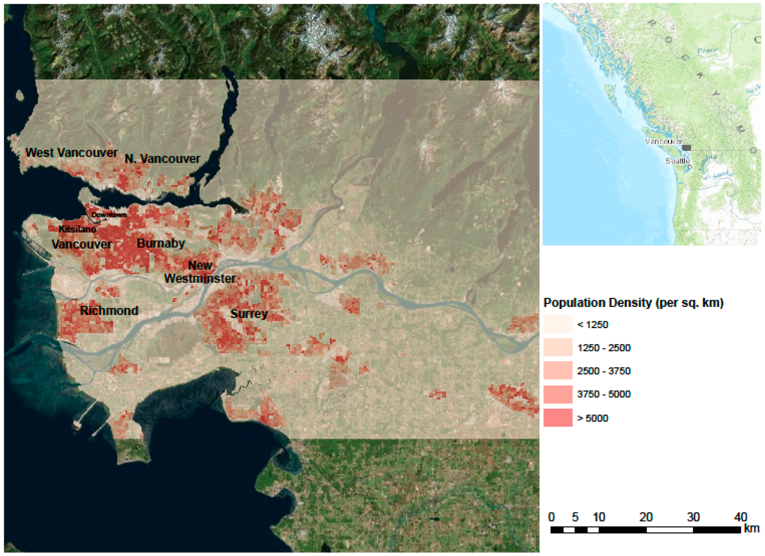
2.1. Study Site
2.2. Data
2.2.1. Vulnerability Data

| Variables Name | Details |
|---|---|
| Seniors | Number of people more than 55 years old |
| Infants | Number of people less than 5 years old |
| People in old houses | Number of households living in housing built prior to 1970 |
| People in high heat risk homes | Number of households living in multi-story apartment buildings or mobile homes |
| Low income population | Number of people with annual household income less than $20,000 |
| Low education population | Number of people without a diploma or a degree |
| People living alone | Number of single-person households |
| Unemployment | Unemployment rate |
2.2.2. Heat Exposure Data
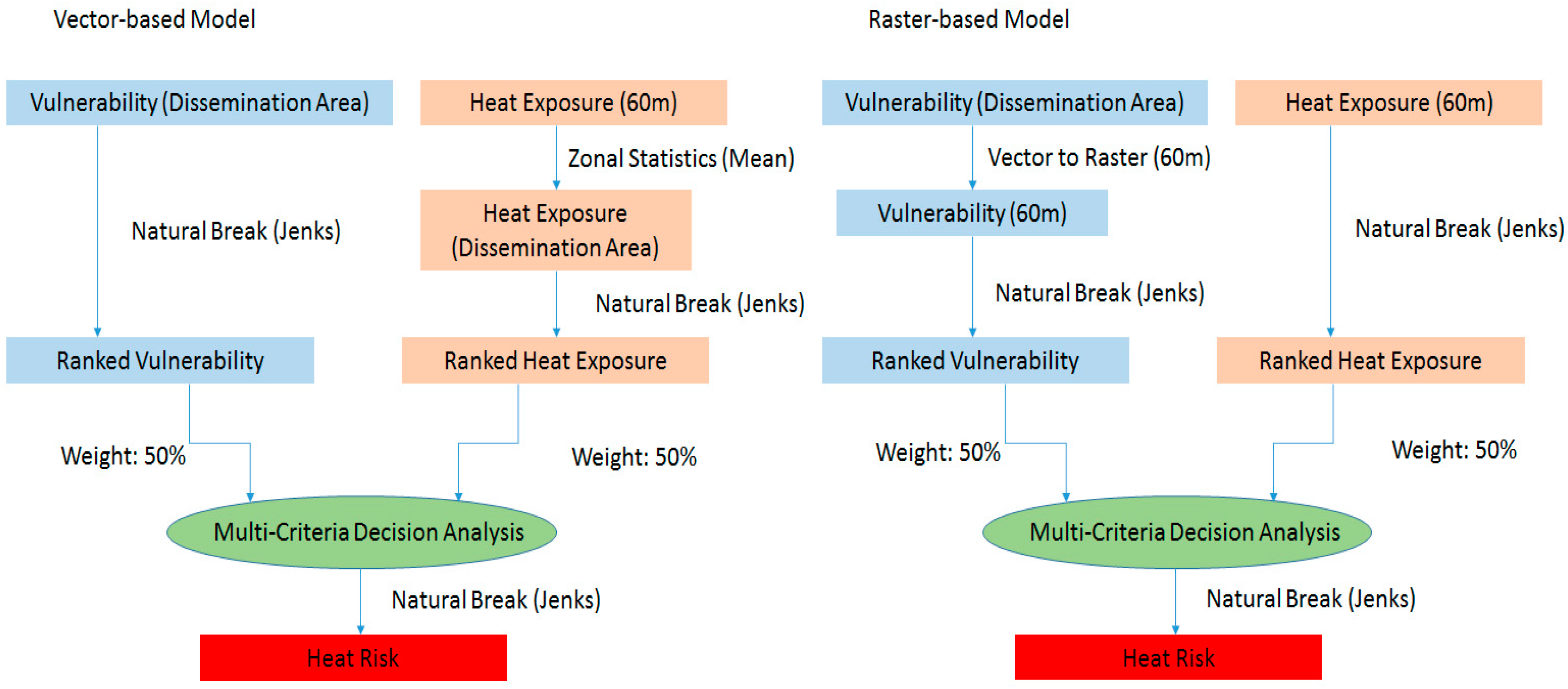
2.3. Multi-Criteria Decision Analysis

2.4. Getis-Ord Gi Index
3. Results
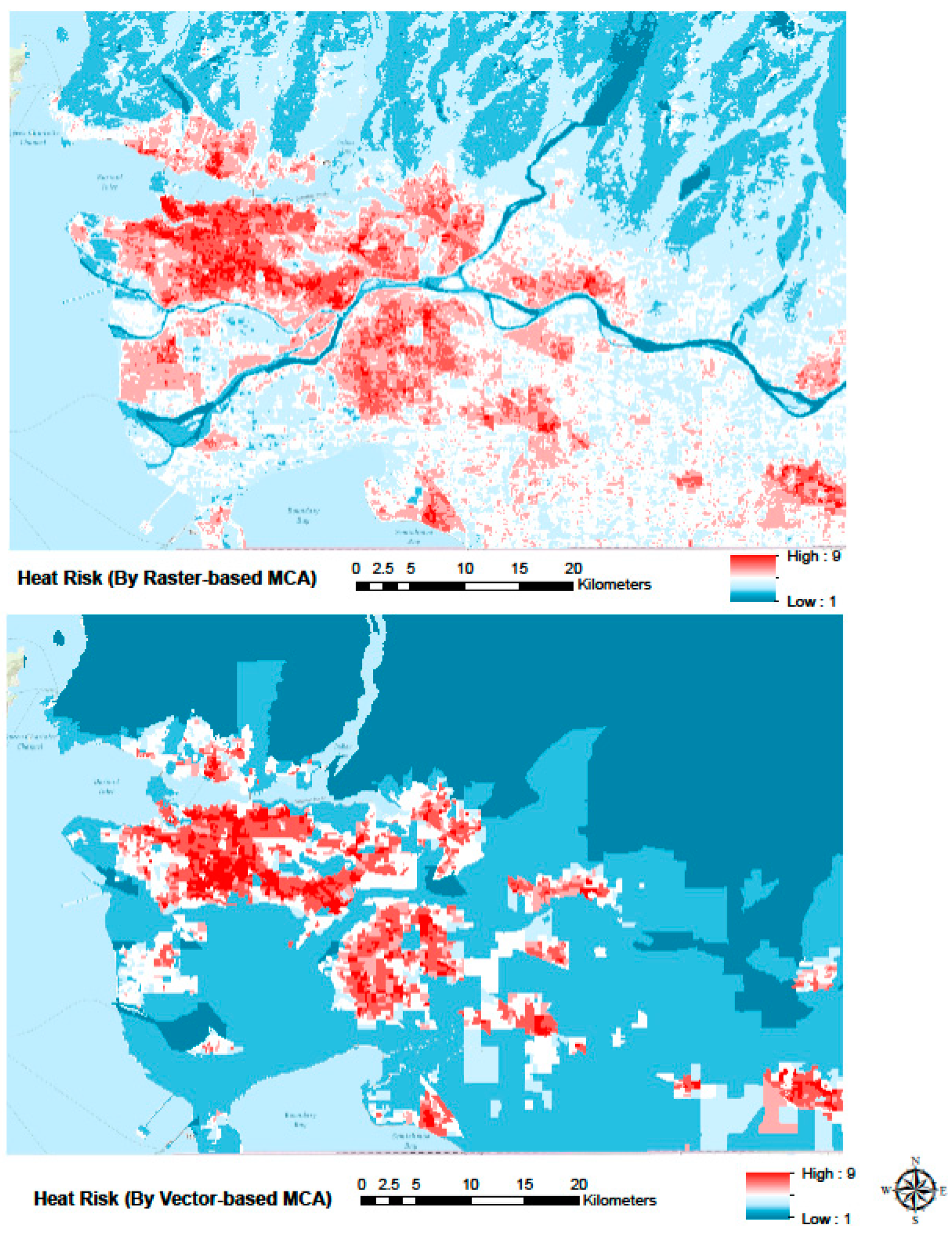
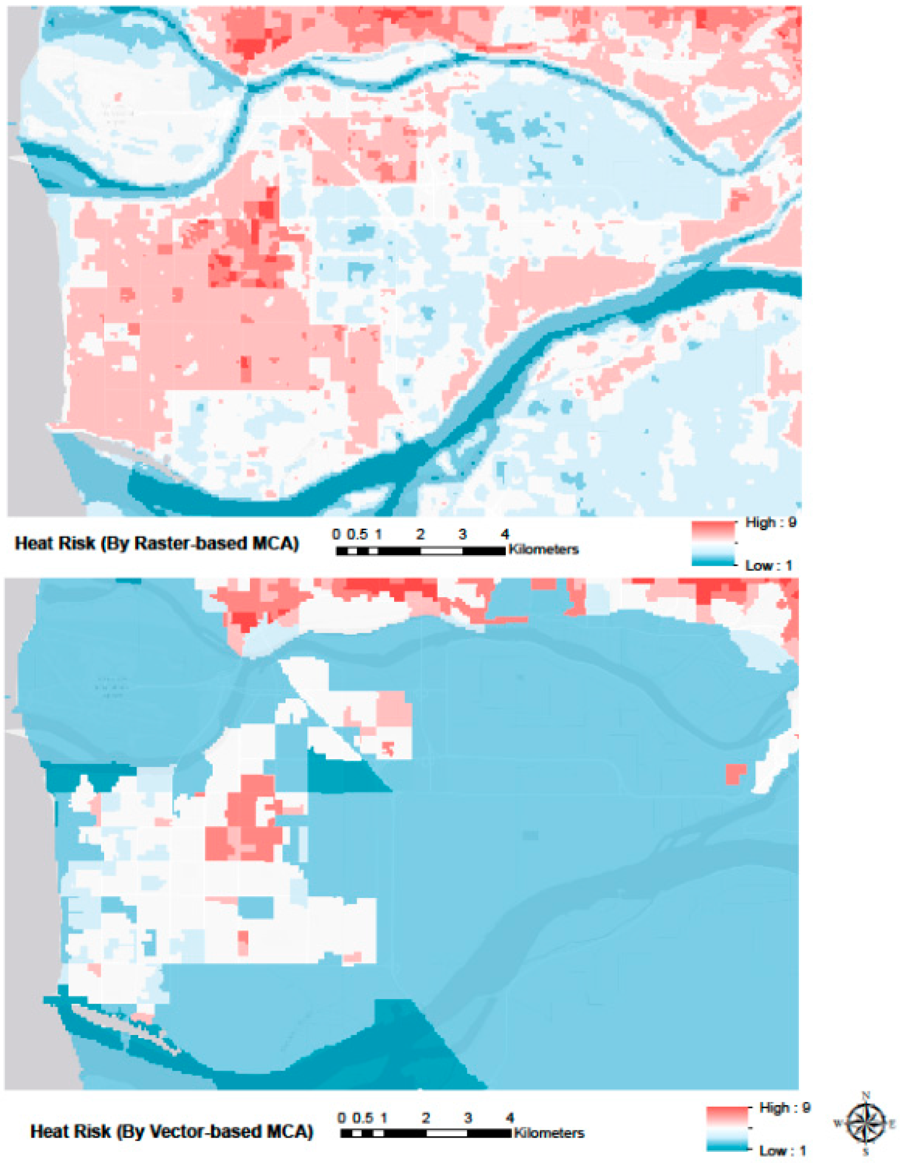
3.1. Raster-Based and Vector-Based Heat Risk Maps

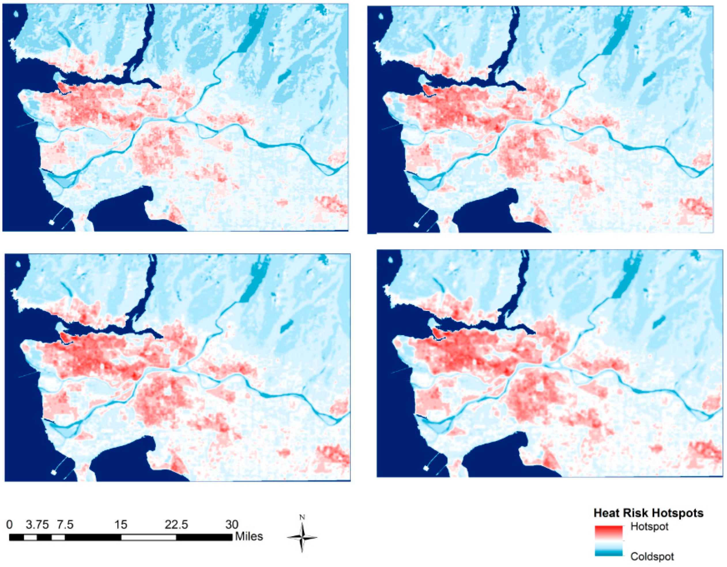
3.2. Multi-Scale Hotspot Analysis

| Risk Category | Mean LST | Mean Seniors | Mean Infants | People in Old Houses | People in High Heat Risk Homes | Low Income Population | Low Education Population | People Living Alone | Unemployment Rate | |
|---|---|---|---|---|---|---|---|---|---|---|
| 1 | Raster-based | 292.4 | 7.2 | 0.8 | 3.1 | 1.3 | 1.3 | 11.4 | 2.1 | 2.1 |
| Vector-based | 299.6 | 6.1 | 0.6 | 1.5 | 1.2 | 0.8 | 7.6 | 1.5 | 2.3 | |
| 2 | Raster-based | 297.9 | 8.4 | 0.9 | 2.6 | 3.3 | 1.4 | 10.0 | 2.6 | 2.4 |
| Vector-based | 305.1 | 57.1 | 6.1 | 22.0 | 18.3 | 10.2 | 77.7 | 17.5 | 3.9 | |
| 3 | Raster-based | 301.8 | 20.6 | 2.0 | 7.6 | 4.8 | 3.0 | 27.9 | 5.3 | 3.1 |
| Vector-based | 308.1 | 227.8 | 25.9 | 85.1 | 63.5 | 33.5 | 323.1 | 62.8 | 4.5 | |
| 4 | Raster-based | 307.0 | 80.3 | 8.2 | 31.2 | 14.8 | 11.3 | 111.2 | 19.3 | 3.9 |
| Vector-based | 309.7 | 496.4 | 61.0 | 215.8 | 136.5 | 86.6 | 745.4 | 140.8 | 6.6 | |
| 5 | Raster-based | 311.3 | 412.4 | 50.6 | 180.2 | 95.2 | 69.6 | 639.0 | 112.0 | 5.4 |
| Vector-based | 312.0 | 599.5 | 79.1 | 307.6 | 235.0 | 122.8 | 967.0 | 210.3 | 5.5 | |
| 6 | Raster-based | 313.1 | 1002.3 | 130.1 | 487.3 | 630.7 | 263.5 | 1637.5 | 434.3 | 7.4 |
| Vector-based | 312.7 | 969.0 | 128.0 | 538.5 | 773.1 | 292.2 | 1556.2 | 522.2 | 6.0 | |
| 7 | Raster-based | 313.3 | 2343.0 | 283.5 | 1505.0 | 3601.6 | 1151.8 | 3578.1 | 2019.4 | 7.9 |
| Vector-based | 313.6 | 1483.9 | 168.6 | 762.1 | 1419.7 | 510.5 | 2450.7 | 860.0 | 7.2 | |
| 8 | Raster-based | 312.6 | 4871.9 | 654.5 | 4788.2 | 11951.1 | 4233.6 | 7317.8 | 6809.0 | 9.0 |
| Vector-based | 314.2 | 2126.5 | 242.9 | 1347.5 | 2979.9 | 1155.6 | 3466.5 | 1705.6 | 8.2 | |
| 9 | Raster-based | 313.9 | 6073.5 | 298.9 | 9284.7 | 14965.3 | 11314.6 | 12507.8 | 12110.7 | 14.8 |
| Vector-based | 314.6 | 4360.7 | 634.0 | 5211.2 | 9453.2 | 4475.1 | 7183.6 | 5847.5 | 8.5 |
4. Discussion
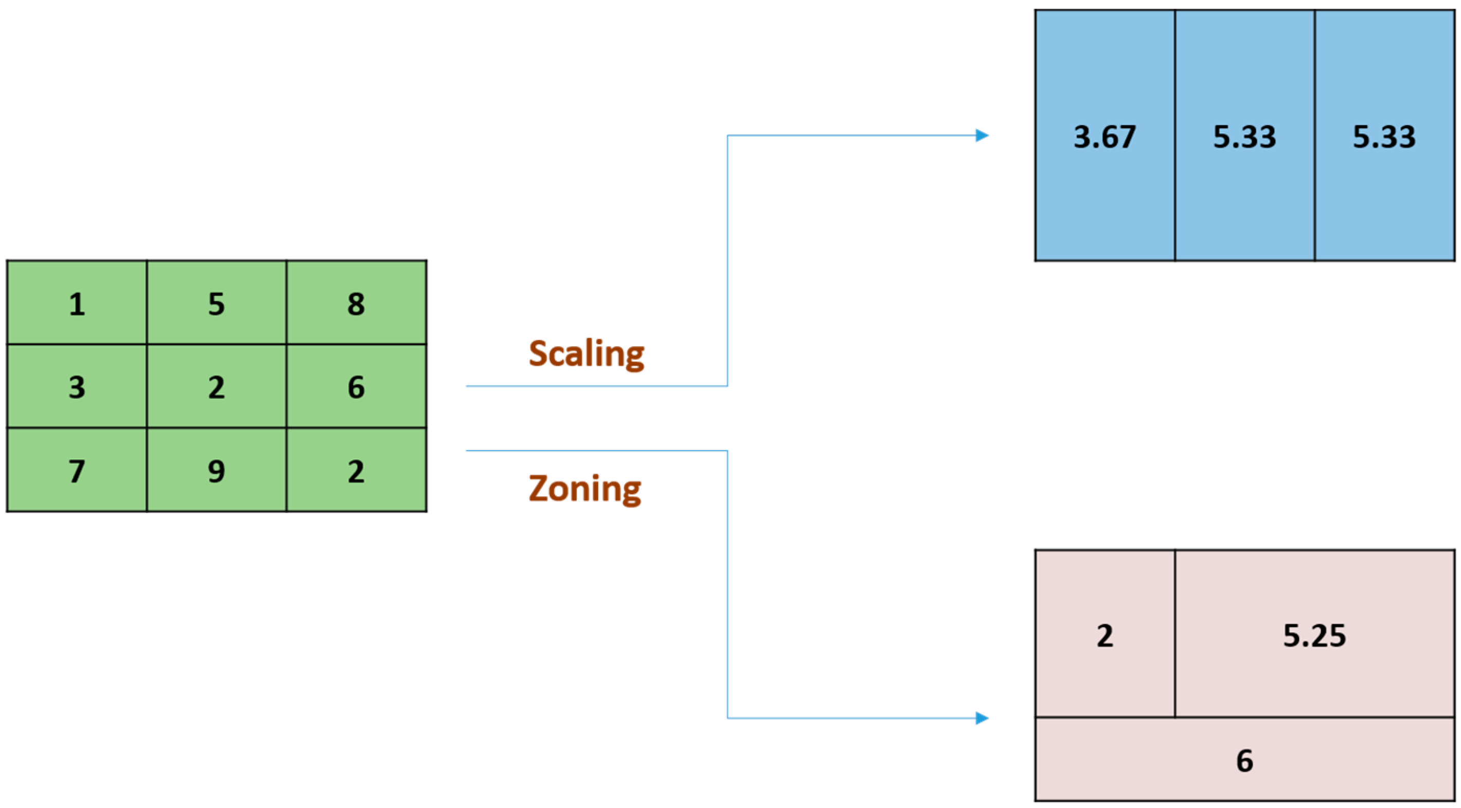
4.1. Comparison of Resampling Approaches
4.2. Multi-Criteria Decision Analysis
4.3. Hotspot Analysis
5. Conclusions
Acknowledgments
Author Contributions
Conflicts of Interest
References
- Meehi, G.A.; Tebaldi, C. More Intense, More Frequent, and Longer Lasting Heat Waves in the 21st Century. Science 2004, 305, 994–997. [Google Scholar]
- Reid, C.E.; O’Neill, M.S.; Gronlund, C.J.; Brines, S.J.; Brown, D.G.; Diez-Roux, A.V.; Schwartz, J. Mapping Community Determinants of Heat Vulnerability. Environ. Health Perspect. 2009, 117, 1730–1736. [Google Scholar] [CrossRef] [PubMed]
- Basu, R. High ambient temperature and mortality: A review of epidemiologic studies from 2001 to 2008. Environ. Health 2009, 8. [Google Scholar] [CrossRef] [PubMed]
- Yan, Y.Y. The influence of weather on human mortality in Hong Kong. Soc. Sci. Med. 2000, 50, 419–427. [Google Scholar] [CrossRef]
- Huang, W.; Kan, H.; Kovats, S. The impact of the 2003 heat wave on mortality in Shanghai, China. Sci. Total Environ. 2010, 408, 2418–2420. [Google Scholar] [CrossRef] [PubMed]
- Filleul, L.; Cassadou, S.; Médina, S.; Fabres, P.; Lefranc, A.; Eilstein, D.; le Tertre, A.; Pascal, L.; Chardon, B.; Blanchard, M.; et al. The relation between temperature, ozone, and mortality in nine French cities during the heat wave of 2003. Environ. Health Perspect. 2006, 114, 1344–1347. [Google Scholar] [CrossRef] [PubMed]
- Fouillet, A.; Rey, G.; Laurent, F.; Pavillon, G.; Bellec, S.; Guihenneuc-Jouyaux, C.; Clavel, J.; Jougla, E.; Hémon, D. Excess mortality related to the August 2003 heat wave in France. Int. Arch. Occup. Environ. Health 2006, 80, 16–24. [Google Scholar] [CrossRef] [PubMed] [Green Version]
- Kosatsky, T.; Henderson, S.B.; Pollock, S.L. Shifts in mortality during a hot weather event in Vancouver, British Columbia: Rapid assessment with case-only analysis. Am. J. Public Health 2012, 102, 2367–2371. [Google Scholar] [CrossRef] [PubMed]
- Baccini, M.; Biggeri, A.; Accetta, G.; Kosatsky, T.; Katsouyanni, K.; Analitis, A.; Anderson, H.R.; Bisanti, L.; D’Ippoliti, D.; Danova, J.; et al. Heat effects on mortality in 15 European cities. Epidemiology 2008, 19, 711–719. [Google Scholar] [CrossRef] [PubMed]
- Curriero, F.C.; Heiner, K.S.; Samet, J.M.; Zeger, S.L.; Strug, L.; Patz, J.A. Temperature and Mortality in 11 Cities of the Eastern United States. Am. J. Epidemiol. 2002, 155, 80–87. [Google Scholar] [CrossRef] [PubMed]
- Zhang, K.; Li, Y.; Schwartz, J.; O’Neill, M. What weather variables are important in predicting heat-related mortality? A new application of statistical learning methods. Environ. Res. 2014, 132, 350–359. [Google Scholar] [CrossRef] [PubMed]
- Morabito, M.; Crisci, A.; Messeri, A.; Capecchi, V.; Modesti, P.A.; Gensini, G.F.; Orlandini, S. Environmental Temperature and Thermal Indices: What is the Most Effective Predictor of Heat-Related Mortality in Different Geographical Contexts? Sci. World. J. 2014, 961750. [Google Scholar] [CrossRef] [PubMed]
- Anderson, G.; Bell, M. Heat Waves in the United States: Mortality Risk during Heat Waves and Effect Modification by Heat Wave Characteristics in 43 U.S. Communities. Environ. Health Perspect. 2011, 119, 210–218. [Google Scholar] [CrossRef] [PubMed]
- Hattis, D.; Ogneva-Himmelberger, Y.; Ratick, S. The spatial variability of heat-related mortality in Massachusetts. Appl. Geogr. 2012, 33, 45–52. [Google Scholar] [CrossRef]
- Henderson, S.; Wan, V.; Kosatsky, T. Differences in heat-related mortality across four ecological regions with diverse urban, rural, and remote populations in British Columbia, Canada. Health Place 2013, 23, 48–53. [Google Scholar] [CrossRef] [PubMed]
- Hondula, D.; Davis, R.; Leisten, M.; Saha, M.; Veazey, L.; Wegner, C. Fine-scale spatial variability of heat-related mortality in Philadelphia County, USA, from 1983 to 2008: A case-series analysis. Environ. Health 2012, 11, 16. [Google Scholar] [CrossRef] [PubMed]
- Jones, T.; Liang, A.; Kilbourne, M.; Griffin, M.; Patriarca, P.; FiteWassilak, S.; Mullan, R.; Herrick, R.; Donnell, H.; Choi, K.; et al. Morbidity and Mortality Associated with the July 1980 Heat Wave in St. Louis and Kansas City, MO. J. Am. Med. Assoc. 1982, 247, 3327–3331. [Google Scholar] [CrossRef]
- Laaidi, K.; Zeghnoun, A.; Dousset, B.; Bretin, P.; Vandentorren, S.; Giraudet, E.; Beaudeau, P. The Impact of Heat Islands on Mortality in Paris during the August 2003 Heat Wave. Environ. Health Perspect. 2012, 120, 254–259. [Google Scholar] [CrossRef] [PubMed]
- Son, J.-Y.; Lee, J.-T.; Anderson, B.; Bell, M.L. The Impact of Heat Waves on Mortality in Seven Major Cities in Korea. Environ. Health Perspect. 2012, 120, 566–571. [Google Scholar] [CrossRef] [PubMed]
- Son, J.-Y.; Lee, J.-T.; Anderson, B.; Bell, M.L. Vulnerability to temperature-related mortality in Seoul, Korea. Environ. Res. Lett. 2012, 6. [Google Scholar] [CrossRef] [PubMed]
- Reid, C.E.; Mann, J.; Alfasso, R.; English, P.B.; King, G.C.; Lincoln, R.A.; Margolis, H.G.; Rubado, D.J.; Sabato, J.E.; West, N.L.; et al. Evaluation of a Heat Vulnerability Index on Abnormally Hot Days: An Environmental Public Health Tracking Study. Environ. Health Perspect. 2012, 120, 715–720. [Google Scholar] [CrossRef] [PubMed]
- Vescovi, L.; Rebetez, M.; Rong, F. Assessing public health risk due to extremely high temperature events: Climate and social parameters. Clim. Res. 2005, 30, 71–78. [Google Scholar] [CrossRef]
- Chuang, W.C.; Gober, P. Predicting hospitalization for heat-related illness at the census tract level: Accuracy of a generic heat vulnerability index in Phoenix, Arizona (USA). Environ. Health Perspect. 2015, 123. [Google Scholar] [CrossRef] [PubMed]
- Buscail, C.; Upegui, E.; Viel, J.-F. Mapping heatwave health risk at the community level for public health action. Int. J. Health Geogr. 2012, 11. [Google Scholar] [CrossRef] [PubMed] [Green Version]
- Tomlinson, C.; Chapman, L.; Thornes, J.; Baker, C. Including the urban heat island in spatial heat health risk assessment strategies: A case study for Birmingham, UK. Int. J. Health Geogr. 2011, 10. [Google Scholar] [CrossRef] [PubMed] [Green Version]
- Morabito, M.; Crisci, A.; Gioli, B.; Gualtieri, G.; Toscano, P.; di Stefano, V.; Gensini, G.F. Urban-Hazard Risk Analysis: Mapping of Heat-Related Risks in the Elderly in Major Italian Cities. PLoS ONE 2015, 10. [Google Scholar] [CrossRef] [PubMed]
- Amrhein, C.G. Searching for the elusive aggregation effect: Evidence from statistical simulations. Environ. Plan. A 1995, 27, 105–119. [Google Scholar] [CrossRef]
- Marceau, D.J. The scale issue in social and natural sciences. Can. J. Remote Sens. 1999, 25, 347–356. [Google Scholar] [CrossRef]
- Marceau, D.J.; Hay, G.J. Remote sensing contributions to the scale issue. Can. J. Remote Sens. 1999, 25, 357–366. [Google Scholar] [CrossRef]
- Schuurman, N.; Bell, N.; Dunn, J.R.; Oliver, L. Deprivation indices, population health and geography: An evaluation of the spatial effectiveness of indices at multiple scales. J. Urban. Health 2007, 84, 591–603. [Google Scholar] [CrossRef] [PubMed]
- Ho, H.C.; Knudby, A.; Sirovyak, P.; Xu, Y.; Hodul, M.; Henderson, S.B. Mapping Maximum Urban Air Temperature on Hot Summer Days. Remote Sens. Environ. 2014, 154, 38–45. [Google Scholar] [CrossRef]
- Sobrino, J.A.; Oltra-Carrió, R.; Sòria, G.; Bianchi, R.; Paganini, M. Impact of spatial resolution and satellite overpass time on evaluation of the surface urban heat island effects. Remote Sens. Environ. 2012, 117, 50–56. [Google Scholar] [CrossRef]
- Xu, Y.; Knudby, A.; Ho, H.C. Estimating daily maximum air temperature from MODIS in British Columbia, Canada. Int. J. Remote Sens. 2014, 35, 8108–8121. [Google Scholar] [CrossRef]
- Statistics Canada. Greater Vancouver, British Columbia (Code5915) (Table). 2006 Community Profiles. 2006 Census; Statistics Canada Catalogue No. 92-591-XWE; Publisher: Ottawa, ON, Canada, Released 13 March 2007.
- Smoyer-Tomic, K.E.; Kuhn, R.; Hudson, A. Heat wave hazards: An overview of heat wave impacts in Canada. Nat. Hazards 2003, 28, 465–486. [Google Scholar] [CrossRef]
- Yardley, J.; Sigal, R.; Kenny, G. Heat health planning: The importance of social and community factors. Glob. Environ. Chang. 2011, 21, 670–679. [Google Scholar] [CrossRef]
- Schifano, P.; Cappai, G.; de Sario, M.D.; Michelozzi, P.; Marino, C.; Bargagli, A.M.; Perucci, C.A. Susceptibility to heat wave-related mortality: A follow-up study of a cohort of elderly in Rome. Environ. Health 2012, 8. [Google Scholar] [CrossRef] [PubMed]
- Tan, J. Commentary: People’s vulnerability to heat wave. Int. J. Epidemiol. 2008, 37, 318–320. [Google Scholar] [CrossRef] [PubMed]
- Flynn, A.; Mcgreevy, C.; Mulkerrin, E. Why do older patients die in a heatwave? QJM Int. J. Med. 2005, 98, 227–229. [Google Scholar] [CrossRef] [PubMed]
- Vandentorren, S.; Bretin, P.; Zeghnoun, A.; Mandereau-Bruno, L.; Croisier, A.; Cochet, C.; Riberon, J.; Siberan, I.; Declercq, B.; Ledrans, M. August 2003 heat wave in France: Risk factors for death of elderly people living at home. Eur. J. Public Health 2006, 16, 583–591. [Google Scholar] [CrossRef] [PubMed]
- Holstein, J.; Canouï-Poitrine, F.; Neumann, A.; Lepage, E.; Spira, A. Were less disabled patients the most affected by 2003 heat wave in nursing homes in Paris, France? J. Public Health 2005, 27, 359–365. [Google Scholar] [CrossRef] [PubMed]
- Danks, D.M.; Webb, D.W.; Allen, J. Heat illness in infants and young children. Br. Med. J. 1962, 2, 287–293. [Google Scholar] [CrossRef] [PubMed]
- Auger, N.; Fraser, W.D.; Smargiassi, A.; Kosatsky, T. Ambient Heat and Sudden Infant Death: A Case-Crossover Study Spanning 30 Years in Montreal, Canada. Environ. Health Perspect. 2015, 123, 712–716. [Google Scholar] [CrossRef] [PubMed]
- McGeehin, M.; Mirabelli, M. The Potential Impacts of Climate Variability and Change on Temperature-Related Morbidity and Mortality in the United States. Environ. Health Perspect. 2001, 109, 185–189. [Google Scholar] [CrossRef] [PubMed]
- Semenza, J.C.; Rubin, C.H.; Falter, K.H.; Selanikio, J.D.; Flanders, W.D.; Howe, H.L.; Wilhelm, J.L. Heat-related deaths during the July 1995 heat wave in Chicago. N. Engl. J. Med. 1996, 335, 84–90. [Google Scholar] [CrossRef] [PubMed]
- Bumbaco, K.A.; Dello, K.D.; Bond, N.A. History of Pacific Northwest heat waves: Synoptic pattern and trends. J. Appl. Meteorol. Climatol. 2013, 52, 1618–1631. [Google Scholar] [CrossRef]
- Acorn, S. Mental and physical health of homeless persons who use emergency shelters in Vancouver. Psychiatr. Serv. 1993, 44, 854–857. [Google Scholar] [CrossRef]
- Gadermann, A.M.; Hubley, A.M.; Russell, L.B.; Palepu, A. Subjective health-related quality of life in homeless and vulnerably housed individuals and its relationship with self-reported physical and mental health status. Soc. Indic. Res. 2014, 116, 341–352. [Google Scholar] [CrossRef]
- Patterson, M.L.; Somers, J.M.; Moniruzzaman, A. Prolonged and persistent homelessness: Multivariable analyses in a cohort experiencing current homelessness and mental illness in Vancouver, British Columbia. Ment. Health Subst. Use 2012, 5, 85–101. [Google Scholar] [CrossRef]
- Naughton, M.P.; Henderson, A.; Mirabelli, M.C.; Kaiser, R.; Wilhelm, J.L.; Kieszak, S.M.; Rubin, C.H.; Mcgeehin, M.A. Heat-related mortality during a 1999 heat wave in Chicago. Am. J. Prevent. Med. 2002, 22, 221–227. [Google Scholar] [CrossRef]
- O’Neill, M.S.; Zanobetti, A.; Schwartz, J. Modifiers of the temperature and mortality association in seven US cities. Am. J. Epidemiol. 2003, 157, 1074–1082. [Google Scholar] [CrossRef] [PubMed]
- O’Neill, M.S.; Zanobetti, A.; Schwartz, J. Disparities by race in heat-related mortality in four US cities: The role of air conditioning prevalence. J. Urban. Health 2005, 82, 191–197. [Google Scholar] [CrossRef] [PubMed]
- Barsi, J.A.; Barker, J.L.; Schott, J.R. An Atmospheric Correction Parameter Calculator for a single thermal band earth-sensing instrument. In Proceedings of the IGARSS IEEE International Geoscience and Remote Sensing Symposium, Toulouse, France, 21–25 July 2003.
- Hulley, G.C.; Hook, S.J. The North American ASTER Land Surface Emissivity Database (NAALSED) version 2.0. Remote Sens. Environ. 2009, 113, 1967–1975. [Google Scholar] [CrossRef]
- Coll, C.; Galve, J.M.; Sánchez, J.M.; Caselles, V. Validation of Landsat-7/ETM+ Thermal-Band Calibration and Atmospheric Corrections with Ground Based Measurements. IEEE Trans. Geosci. Remote Sens. 2010, 48, 547–555. [Google Scholar] [CrossRef]
- Chi, G. Land developability: Developing an index of land use and development for population research. J. Maps 2010, 6, 609–617. [Google Scholar] [CrossRef]
- Ho, H.C.; Mylroie, J.; Infante, L.; Rodgers, J. Fuzzy-based Spatial Modeling Approach to Predict Island Karst Distribution. Environ. Earth Sci. 2014, 71, 1369–1377. [Google Scholar] [CrossRef]
- Crichton, D. The risk triangle. In Natural Disaster Management; Ingleton, J., Ed.; Tudor Rose: London, UK, 1999; pp. 102–103. [Google Scholar]
- Jenks, G. The Data Model Concept in Statistical Mapping. Int. Yearb. Cartogr. 1967, 7, 186–190. [Google Scholar]
- Getis, A.; Ord, J.K. The analysis of spatial association by use of distance statistics. Geogr. Anal. 1992, 24, 189–206. [Google Scholar] [CrossRef]
- Lanorte, A.; Danese, M.; Lasaponara, R.; Murgante, B. Multiscale mapping of burn area and severity using multisensor satellite data and spatial autocorrelation analysis. Int. J. Appl. Earth Obs. Geoinform. 2013, 20, 42–51. [Google Scholar] [CrossRef]
- Hansen, A.; Bi, L.; Saniotis, A.; Nitschke, M. Vulnerability to extreme heat and climate change: Is ethnicity a factor? Glob. Health Action 2013, 6. [Google Scholar] [CrossRef] [PubMed] [Green Version]
- Bell, N.; Hayes, M.V. The Vancouver Area Neighbourhood Deprivation Index (Vandix): A census-based tool for assessing small-area variations in health status. Can. J. Public Health Rev. Can. Santé Publique 2012, 103, S28–S32. [Google Scholar]
- Höppe, P. The physiological equivalent temperature—A universal index for the biometeorological assessment of the thermal environment. Int. J. Biometeorol. 1999, 43, 71–75. [Google Scholar] [PubMed]
- Matzarakis, A.; Mayer, H.; Iziomon, M.G. Applications of a universal thermal index: Physiological equivalent temperature. Int. J. Biometeorol. 1999, 43, 76–84. [Google Scholar] [CrossRef] [PubMed]
- Nichol, J.E.; To, P.H. Temporal characteristics of thermal satellite images for urban heat stress and heat island mapping. ISPRS J. Photogramm. Remote Sens. 2012, 74, 153–162. [Google Scholar] [CrossRef]
© 2015 by the authors; licensee MDPI, Basel, Switzerland. This article is an open access article distributed under the terms and conditions of the Creative Commons by Attribution (CC-BY) license (http://creativecommons.org/licenses/by/4.0/).
Share and Cite
Ho, H.C.; Knudby, A.; Huang, W. A Spatial Framework to Map Heat Health Risks at Multiple Scales. Int. J. Environ. Res. Public Health 2015, 12, 16110-16123. https://doi.org/10.3390/ijerph121215046
Ho HC, Knudby A, Huang W. A Spatial Framework to Map Heat Health Risks at Multiple Scales. International Journal of Environmental Research and Public Health. 2015; 12(12):16110-16123. https://doi.org/10.3390/ijerph121215046
Chicago/Turabian StyleHo, Hung Chak, Anders Knudby, and Wei Huang. 2015. "A Spatial Framework to Map Heat Health Risks at Multiple Scales" International Journal of Environmental Research and Public Health 12, no. 12: 16110-16123. https://doi.org/10.3390/ijerph121215046