
Developing a Heatwave Early Warning System for Sweden: Evaluating Sensitivity of Different Epidemiological Modelling Approaches to Forecast Temperatures

Abstract
:1. Introduction
2. Experimental Section
2.1. Data
2.2. Study Design
3. Results and Discussion
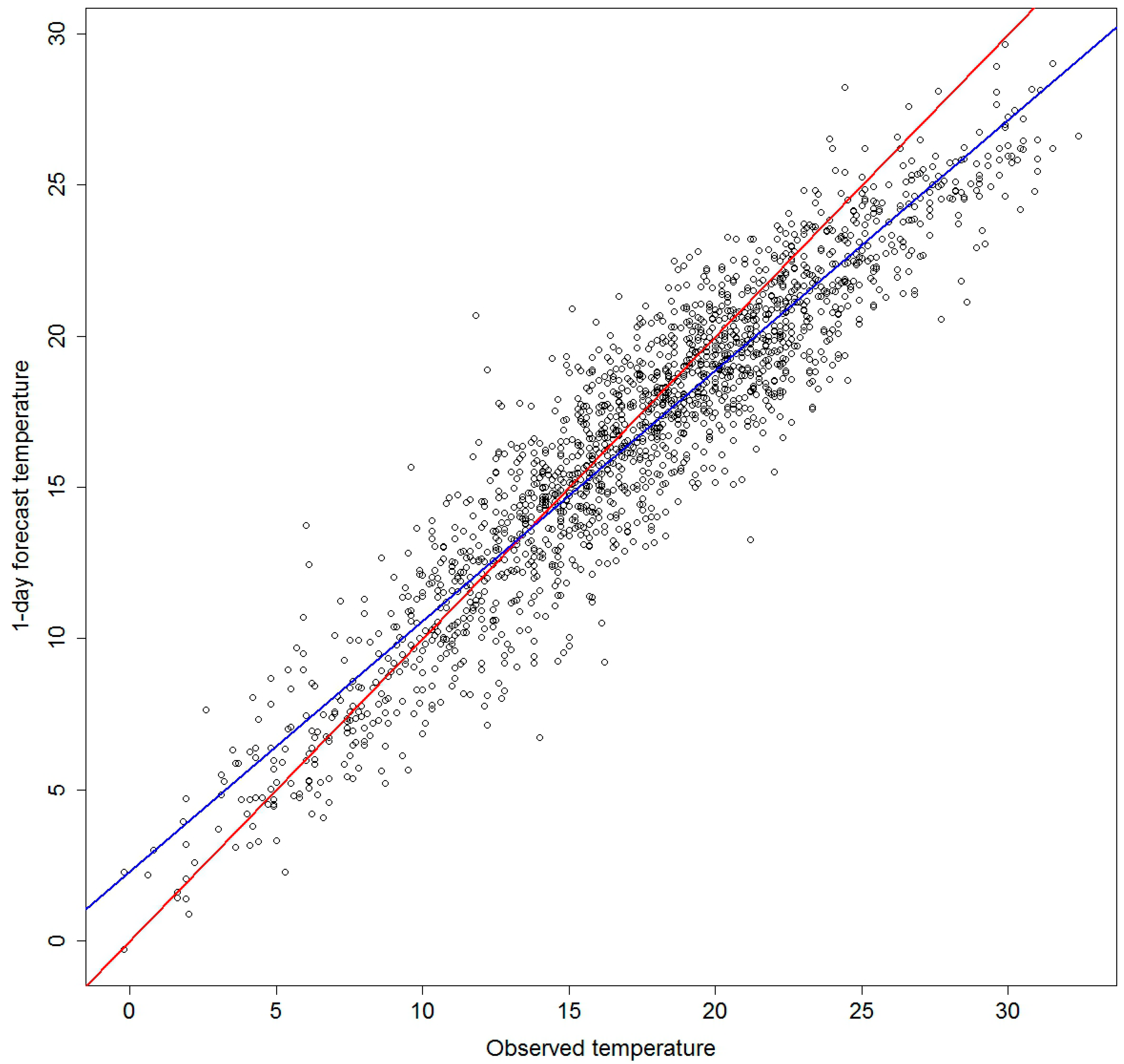
3.1. Forecasts

| Forecast Length | Intercept | Slope |
|---|---|---|
| 1-day forecast | 2.283 | 0.829 |
| 2-day forecast | 2.388 | 0.825 |
| 3-day forecast | 2.753 | 0.795 |
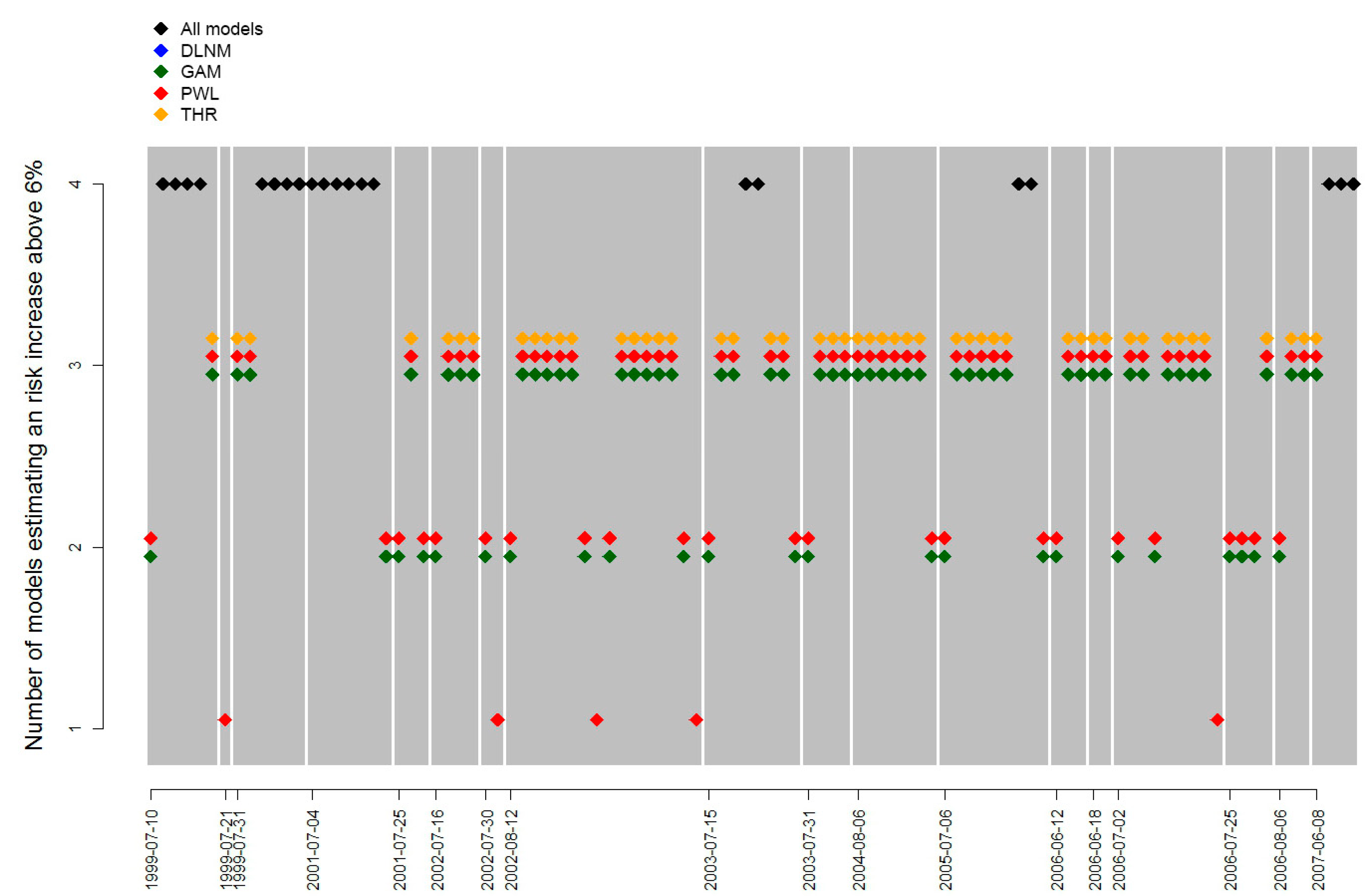
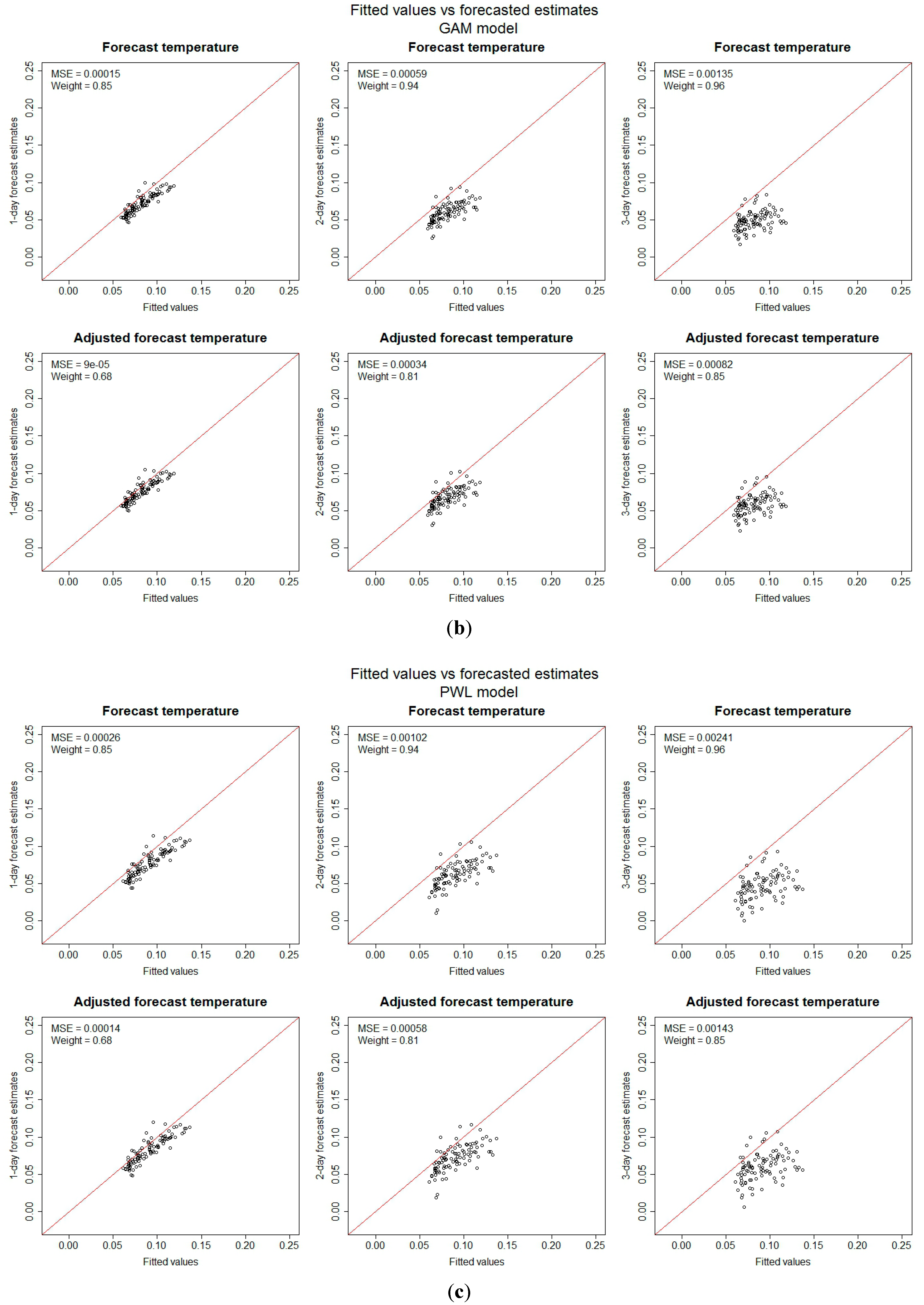
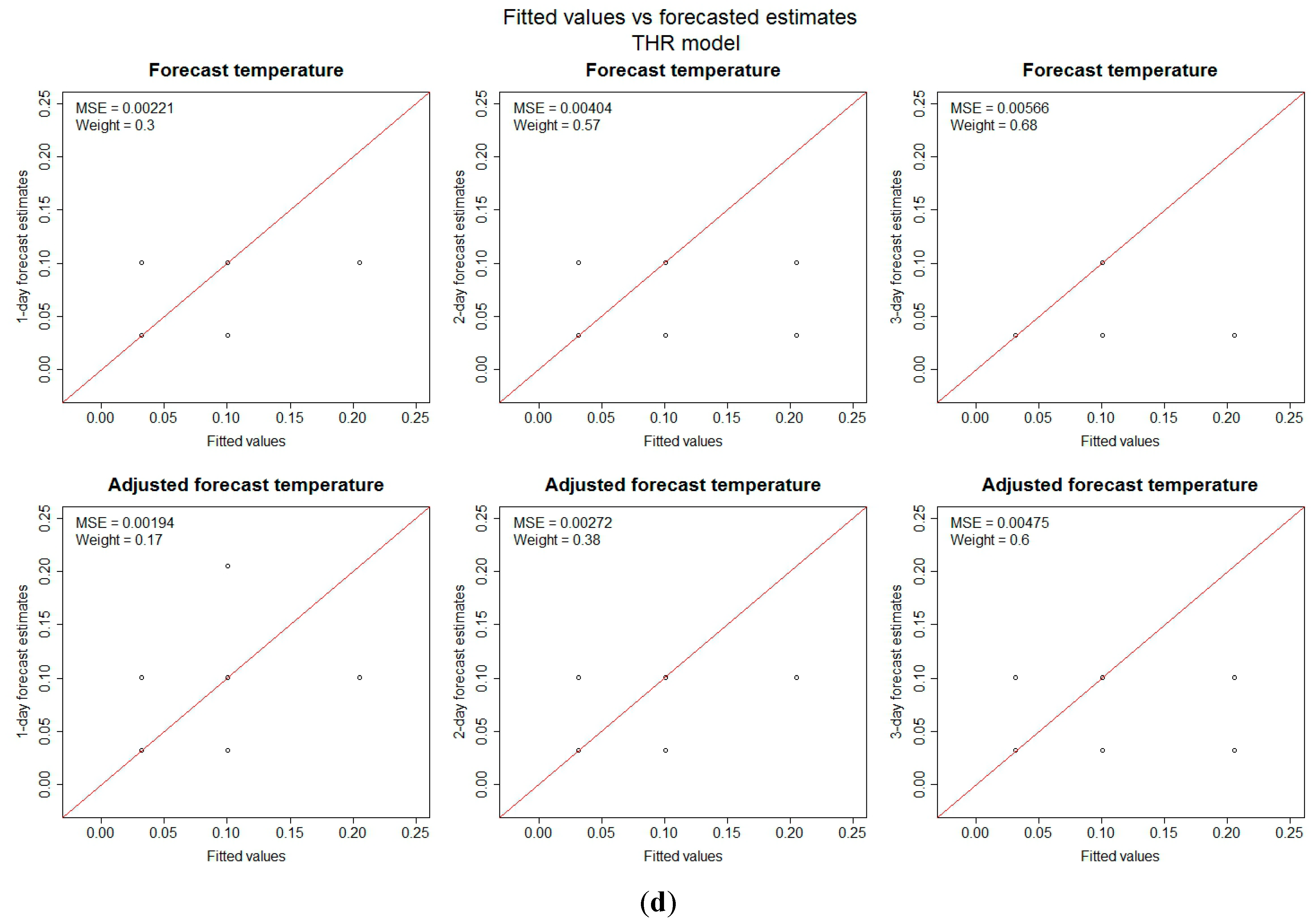
3.2. Risk Models

| Model Type | Forecast | Adjusted Forecast | ||||
|---|---|---|---|---|---|---|
| 1-day | 2-day | 3-day | 1-day | 2-day | 3-day | |
| DLNM | 0.62 | 0.05 | NA | 0.67 | 0.10 | NA |
| GAM | 0.78 | 0.53 | 0.16 | 0.86 | 0.72 | 0.41 |
| PWL | 0.79 | 0.56 | 0.19 | 0.88 | 0.72 | 0.47 |
| THR | 0.70 | 0.30 | 0.09 | 0.84 | 0.57 | 0.23 |
| Model Type | Forecast | Adjusted Forecast | ||||
|---|---|---|---|---|---|---|
| 1-day | 2-day | 3-day | 1-day | 2-day | 3-day | |
| DLNM | 1.00 | 1.00 | NA | 0.88 | 0.50 | NA |
| GAM | 1.00 | 0.98 | 0.94 | 0.99 | 0.94 | 0.93 |
| PWL | 1.00 | 1.00 | 1.00 | 0.98 | 0.97 | 0.93 |
| THR | 0.96 | 0.95 | 1.00 | 0.97 | 0.91 | 0.89 |


4. Discussion
5. Conclusions
Acknowledgments
Author Contributions
Conflicts of Interest
References
- Semenza, J.C.; Rubin, C.H.; Falter, K.H.; Selanikio, J.D.; Flanders, W.D.; Howe, H.L.; Wilhelm, J.L. Heat-related deaths during the July 1995 heat wave in Chicago. N. E. J. Med. 1996, 335, 84–90. [Google Scholar] [CrossRef]
- Fouillet, A.; Rey, G.; Laurent, F.; Pavillon, G.; Bellec, S.; Guihenneuc-Jouyaux, C.; Clavel, J.; Jougla, E.; Hemon, D. Excess mortality related to the august 2003 heat wave in France. Int. Arch. Occup. Environ. Health 2006, 80, 16–24. [Google Scholar] [CrossRef] [PubMed] [Green Version]
- Shaposhnikov, D.; Revich, B.; Bellander, T.; Bedada, G.B.; Bottai, M.; Kharkova, T.; Kvasha, E.; Lezina, E.; Lind, T.; Semutnikova, E.; et al. Mortality related to air pollution with the Moscow heat wave and wildfire of 2010. Epidemiology 2014, 25, 359–364. [Google Scholar] [CrossRef] [PubMed]
- Lowe, D.; Ebi, K.L.; Forsberg, B. Heatwave early warning systems and adaptation advice to reduce human health consequences of heatwaves. Int. J. Environ. Res. Public Health 2011, 8, 4623–4648. [Google Scholar] [CrossRef] [PubMed]
- Metzger, K.B.; Ito, K.; Matte, T.D. Summer heat and mortality in new york city: How hot is too hot? Environ. Health Persp. 2010, 118, 80–86. [Google Scholar]
- Hajat, S.; Armstrong, B.; Baccini, M.; Biggeri, A.; Bisanti, L.; Russo, A.; Paldy, A.; Menne, B.; Kosatsky, T. Impact of high temperatures on mortality—Is there an added heat wave effect? Epidemiology 2006, 17, 632–638. [Google Scholar] [CrossRef] [PubMed]
- Barnett, A.G.; Tong, S.; Clements, A.C.A. What measure of temperature is the best predictor of mortality? Environ. Res. 2010, 110, 604–611. [Google Scholar] [CrossRef] [PubMed] [Green Version]
- Morabito, M.; Crisci, A.; Messeri, A.; Capecchi, V.; Modesti, P.A.; Gensini, G.F.; Orlandini, S. Environmental temperature and thermal indices: What is the most effective predictor of heat-related mortality in different geographical contexts? Sci. World J. 2014, 2014. [Google Scholar] [CrossRef]
- Baccini, M.; Biggeri, A.; Accetta, G.; Kosatsky, T.; Katsouyanni, K.; Analitis, A.; Anderson, H.R.; Bisanti, L.; D’Ippoliti, D.; Danova, J.; et al. Heat effects on mortality in 15 European cities. Epidemiology 2008, 19, 711–719. [Google Scholar] [CrossRef] [PubMed]
- Rocklov, J.; Forsberg, B. The effect of temperature on mortality in Stockholm 1998–2003: A study of lag structures and heatwave effects. Scand. J. Public Health 2008, 36, 516–523. [Google Scholar] [CrossRef] [PubMed]
- Guo, Y.M.; Barnett, A.G.; Pan, X.C.; Yu, W.W.; Tong, S.L. The impact of temperature on mortality in tianjin, china: A case-crossover design with a distributed lag nonlinear model. Environ. Health Persp. 2011, 119, 1719–1725. [Google Scholar] [CrossRef] [Green Version]
- Hajat, S.; Armstrong, B.G.; Gouveia, N.; Wilkinson, P. Mortality displacement of heat-related deaths: A comparison of delhi, Sao Paulo, and London. Epidemiology 2005, 16, 613–620. [Google Scholar] [CrossRef]
- Gasparrini, A. Distributed lag linear and non-linear models in R: The package dlnm. J. Stat. Softw. 2011, 43, 1–20. [Google Scholar] [PubMed]
- Wood, S.N. Generalized Additive Models : An Introduction with R; Chapman & Hall/CRC: Boca Raton, FL, USA, 2006; p. 391. [Google Scholar]
- Zhang, K.; Chen, Y.H.; Schwartz, J.D.; Rood, R.B.; O’Neill, M.S. Using forecast and observed weather data to assess performance of forecast products in identifying heat waves and estimating heat wave effects on mortality. Environ. Health Perspect. 2014, 122, 912–918. [Google Scholar] [PubMed]
- Morabito, M.; Profili, F.; Crisci, A.; Francesconi, P.; Gensini, G.F.; Orlandini, S. Heat-related mortality in the florentine area (Italy) before and after the exceptional 2003 heat wave in europe: An improved public health response? Int. J. Biometeorol. 2012, 56, 801–810. [Google Scholar] [CrossRef] [PubMed]
© 2014 by the authors; licensee MDPI, Basel, Switzerland. This article is an open access article distributed under the terms and conditions of the Creative Commons Attribution license (http://creativecommons.org/licenses/by/4.0/).
Share and Cite
Åström, C.; Ebi, K.L.; Langner, J.; Forsberg, B. Developing a Heatwave Early Warning System for Sweden: Evaluating Sensitivity of Different Epidemiological Modelling Approaches to Forecast Temperatures. Int. J. Environ. Res. Public Health 2015, 12, 254-267. https://doi.org/10.3390/ijerph120100254
Åström C, Ebi KL, Langner J, Forsberg B. Developing a Heatwave Early Warning System for Sweden: Evaluating Sensitivity of Different Epidemiological Modelling Approaches to Forecast Temperatures. International Journal of Environmental Research and Public Health. 2015; 12(1):254-267. https://doi.org/10.3390/ijerph120100254
Chicago/Turabian StyleÅström, Christofer, Kristie L. Ebi, Joakim Langner, and Bertil Forsberg. 2015. "Developing a Heatwave Early Warning System for Sweden: Evaluating Sensitivity of Different Epidemiological Modelling Approaches to Forecast Temperatures" International Journal of Environmental Research and Public Health 12, no. 1: 254-267. https://doi.org/10.3390/ijerph120100254