Comparing Multipollutant Emissions-Based Mobile Source Indicators to Other Single Pollutant and Multipollutant Indicators in Different Urban Areas

 ,
,
Abstract
:1. Introduction
2. Methods
2.1. Urban Areas
2.2. Air Quality Data

| Urban Area | Site | County | Study Period | Monitoring Network | Measurement Methods |
|---|---|---|---|---|---|
| Atlanta, GA | Jefferson Street (JST) Central-site | Fulton (JST) | 2005–2010 | SEARCH | CHL (NOx) |
| NDIR (CO) | |||||
| TOR (EC, BC, OC) | |||||
| IC (ions) | |||||
| AC (NH4+) | |||||
| XRF (trace elements) | |||||
| Atlanta, GA | South Dekalb (SD) Secondary Site | Dekalb (SD) | 2005–2010 | AQS | CHL (NOx) * |
| NDIR (CO) | |||||
| TOR (EC) | |||||
| IC (ions) | |||||
| XRF (trace elements) | |||||
| Denver, CO | Palmer (PAL) * Central-site | Denver (PAL) | 2004–2005 | AQS | CHL (NOx) ** |
| NDIR (CO) | |||||
| TOT (EC,OC) | |||||
| IC (ions) | |||||
| Denver, CO | Alsup (ALS) ** Secondary Site | Adams (ALS) | 2004–2005 | AQS | CHL (NOx) * |
| NDIR (CO) | |||||
| TOR (EC) | |||||
| IC (ions) | |||||
| XRF (trace elements) | |||||
| Houston, TX | Aldine (AL) Central-site | Houston (AL) | 2003–2005 | AQS | CHL (NOx) * |
| NDIR (CO) | |||||
| TOR (EC) | |||||
| IC (ions) | |||||
| XRF (trace elements) | |||||
| Houston, TX | Deer Park (DP) Secondary Site | Houston (DP) | 2003–2005 | AQS | CHL (NOx) * |
| NDIR (CO) | |||||
| TOR (EC) | |||||
| IC (ions) | |||||
| XRF (trace elements) |
2.3. Single Pollutant Metrics
2.4. Multipollutant Metrics: Source Apportionment Factors
| Urban Area | Avg | SD | CV | Min | 10 | 25 | 50 | 75 | 90 | 100 | N |
|---|---|---|---|---|---|---|---|---|---|---|---|
| 1-h max NOx+, ppb (24 h avg.) | |||||||||||
| Atlanta | 89.2 | 58.8 | 0.66 | 15.9 | 25.4 | 41.6 | 75.0 | 128.1 | 170.5 | 305.5 | 257 |
| (38.7) | (27.2) | (0.70) | (7.0) | (15.1) | (20.6) | (31.4) | (47.8) | (71.4) | (169.1) | (257) | |
| Denver + | 42.0 | 11.3 | 0.27 | 15.0 | 27.0 | 33.0 | 42.0 | 50.0 | 57.0 | 81.0 | 260 |
| (25.2) | (9.1) | (0.36) | (4.2) | (13.0) | (18.2) | (25.7) | (32.0) | (40.0) | (50.0) | (260) | |
| Houston | 62.3 | 49.9 | 0.80 | 4.0 | 20.0 | 30.0 | 47.0 | 79.0 | 130.0 | 327.0 | 348 |
| (21.4) | (15.0) | (0.70) | (0.6) | (9.3) | (12.7) | (17.1) | (25.2) | (38.1) | (112.1) | (348) | |
| 1-h max CO, ppm (24 h avg.) | |||||||||||
| Atlanta | 0.86 | 0.65 | 0.76 | 0.17 | 0.31 | 0.39 | 0.65 | 1.06 | 1.87 | 4.09 | 365 |
| (0.44) | (0.22) | (0.55) | (0.13) | (0.22) | (0.27) | (0.33) | (0.47) | (0.67) | (1.82) | (365) | |
| Denver | 0.73 | 1.45 | 1.99 | 0.40 | 0.70 | 1.00 | 1.20 | 1.70 | 2.50 | 4.60 | 363 |
| (0.70) | (0.26) | (0.37) | (0.31) | (0.47) | (0.53) | (0.64) | (0.79) | (1.08) | (1.94) | (363) | |
| Houston | 0.88 | 0.48 | 0.55 | 0.00 | 0.40 | 0.50 | 0.70 | 1.10 | 1.64 | 2.80 | 365 |
| (0.45) | (0.15) | (0.33) | (0.00) | (0.31) | (0.36) | (0.43) | (0.52) | (0.63) | (1.19) | (365) | |
| EC, μg/m3 | |||||||||||
| Atlanta | 1.49 | 0.94 | 0.63 | 0.21 | 0.55 | 0.84 | 1.26 | 1.96 | 2.70 | 6.63 | 350 |
| Denver | 0.51 | 0.30 | 0.59 | 0.04 | 0.22 | 0.32 | 0.47 | 0.61 | 0.82 | 2.09 | 272 |
| Houston | 0.72 | 0.44 | 0.61 | 0.01 | 0.24 | 0.46 | 0.66 | 0.91 | 1.24 | 3.25 | 101 |
| IMSIGV * | |||||||||||
| Atlanta | 1.5 | 1.0 | 0.67 | 0.3 | 0.5 | 0.7 | 1.2 | 2.0 | 3.0 | 5.4 | 257 |
| Denver | 2.2 | 0.6 | 0.30 | 0.7 | 1.5 | 1.7 | 2.1 | 2.5 | 3.0 | 4.9 | 260 |
| Houston | 1.5 | 0.9 | 0.60 | 0.3 | 0.7 | 0.9 | 1.3 | 1.8 | 2.9 | 5.6 | 335 |
| IMSIDV * | |||||||||||
| Atlanta | 1.5 | 0.9 | 0.58 | 0.3 | 0.6 | 0.8 | 1.3 | 2.0 | 2.8 | 5.4 | 244 |
| Denver | 2.1 | 0.8 | 0.36 | 0.7 | 1.3 | 1.6 | 2.0 | 2.5 | 3.0 | 6.0 | 257 |
| Houston | 0.8 | 0.5 | 0.62 | 0.1 | 0.3 | 0.5 | 0.7 | 1.0 | 1.5 | 3.9 | 98 |
| IMSIEB * | |||||||||||
| Atlanta | 1.5 | 0.9 | 0.60 | 0.3 | 0.6 | 0.8 | 1.3 | 2.0 | 2.8 | 5.3 | 244 |
| Denver | 2.1 | 0.7 | 0.31 | 0.7 | 1.3 | 1.6 | 2.0 | 2.4 | 2.9 | 5.3 | 257 |
| Houston | 1.5 | 0.9 | 0.57 | 0.5 | 0.7 | 0.9 | 1.3 | 1.9 | 2.7 | 6.1 | 94 |
| PMFGV, μg/m3 | |||||||||||
| Atlanta | 1.4 | 1.1 | 0.75 | −0.3 | 0.5 | 0.8 | 1.1 | 1.8 | 2.8 | 7.6 | 344 |
| Denver | 0.2 | 0.1 | 0.44 | 0.0 | 0.1 | 0.1 | 0.2 | 0.3 | 0.3 | 0.7 | 272 |
| Houston | 3.5 | 2.0 | 0.58 | −0.7 | 1.1 | 2.2 | 3.6 | 4.7 | 6.0 | 13.0 | 92 |
| PMFDV, μg/m3 | |||||||||||
| Atlanta | 2.3 | 2.0 | 0.84 | −0.5 | 0.4 | 0.9 | 2.0 | 3.1 | 4.8 | 13.6 | 344 |
| Denver | 1.1 | 0.8 | 0.71 | 0.0 | 0.3 | 0.6 | 0.9 | 1.4 | 1.9 | 5.0 | 272 |
| Houston | 1.1 | 0.8 | 0.75 | −0.2 | 0.3 | 0.6 | 0.9 | 1.5 | 2.1 | 5.7 | 92 |
| PMFMB, μg/m3 | |||||||||||
| Atlanta | 3.8 | 2.6 | 0.69 | 0.4 | 1.3 | 1.9 | 3.1 | 4.8 | 7.2 | 21.2 | 344 |
| Denver | 1.3 | 0.8 | 0.61 | 0.1 | 0.5 | 0.8 | 1.2 | 1.6 | 2.1 | 5.3 | 272 |
| Houston | 4.6 | 2.5 | 0.54 | 0.0 | 1.9 | 3.1 | 4.3 | 5.9 | 7.3 | 18.7 | 92 |
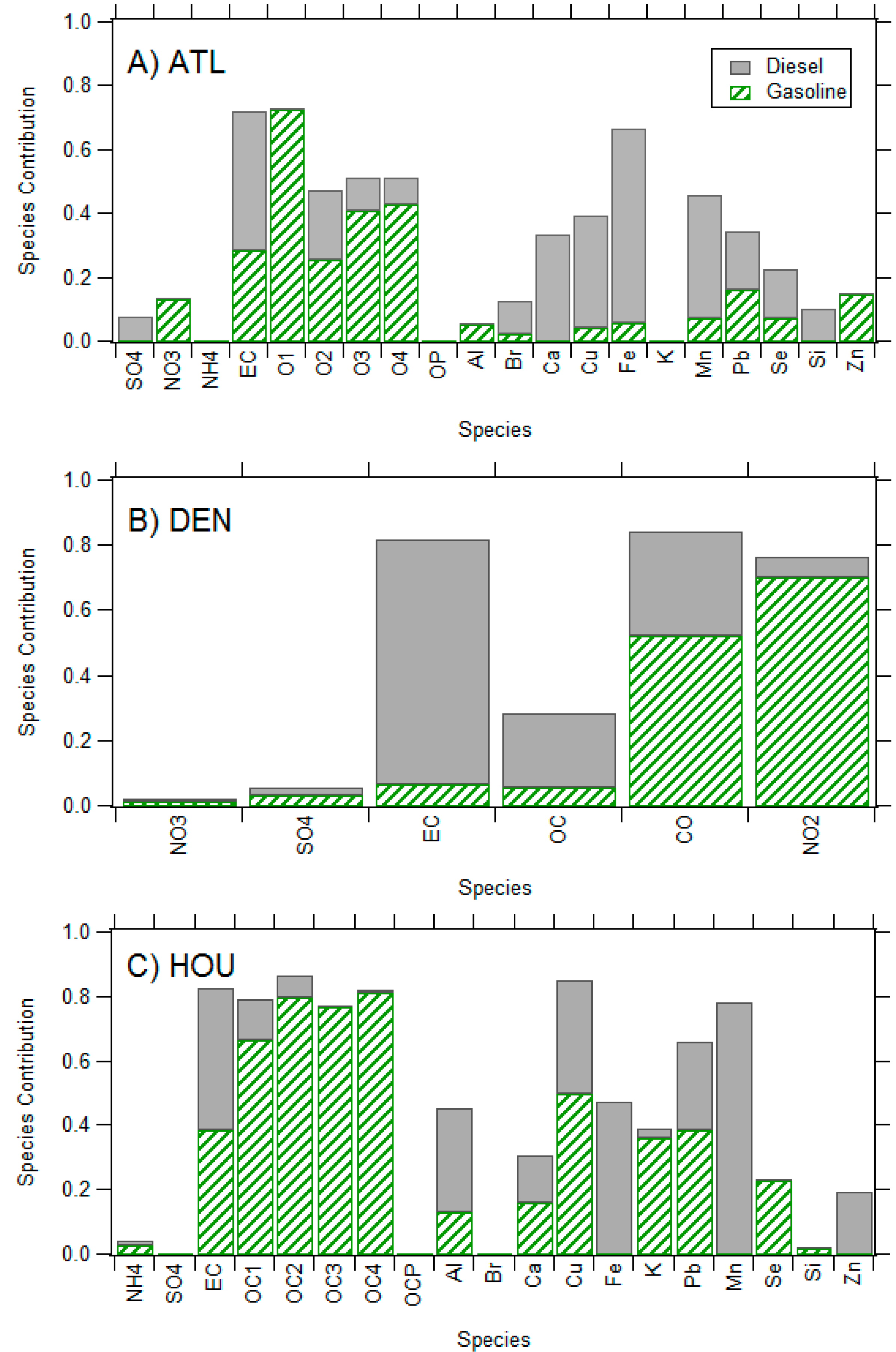
| Urban Area (Monitoring Site) | PMF Version | Input Species | Factor (% Contribution of Pollutant Mass) |
|---|---|---|---|
| Atlanta (Jefferson Street) | PMF3.0 | SO42−, NO3−, NH4+, EC, OC1, OC2, OC3, OC4, OP, Al, Br, Ca, Cu, Fe, K, Mn, Pb, Se, Si, Zn | Diesel vehicle (10.8%) |
| Gasoline vehicle (14.9%) | |||
| Zinc (1.8%) | |||
| Dust (1.6%) | |||
| Sec NH4+ (17.8%) | |||
| Biomass Burning (6.6%) | |||
| NO3− (6.8%) | |||
| SO42−, NH4+ (39.6%) | |||
| Denver (Palmer) | PMF2 | NO3−, SO42−, EC, OC, CO, NO2 | EC/Diesel (19.6%) |
| Trace Gas/Gasoline (5.5%) | |||
| NO3− (15.3%) | |||
| SO42− (22.4%) | |||
| OC (37.2%) | |||
| Houston (Aldine) | PMF5.0 | SO42−, NH4+, EC. OC1, OC2, OC3, OC4, Al, Br Ca, Cu, Fe, K, Mn, Pb, Se, Si, Zn | Diesel (7.7%) |
| Gasoline (25%) | |||
| Zinc-rich (0.6%) | |||
| Dust/soil (12.2%) | |||
| SO42− (38.6%) | |||
| Biomass Burning (16%) |
2.5. Multipollutant Indicators: Emission-Based Integrated Mobile Source Indicators (IMISI)
2.6. Spatial and Temporal Comparison of Metrics in Different Urban Locations
3. Results
3.1. Concentrations of Central-Site Single Pollutant and Multipollutant Metrics
3.2. Characteristics of Multipollutant Metrics in Different Urban Locations
3.2.1. Source Apportionment Factors

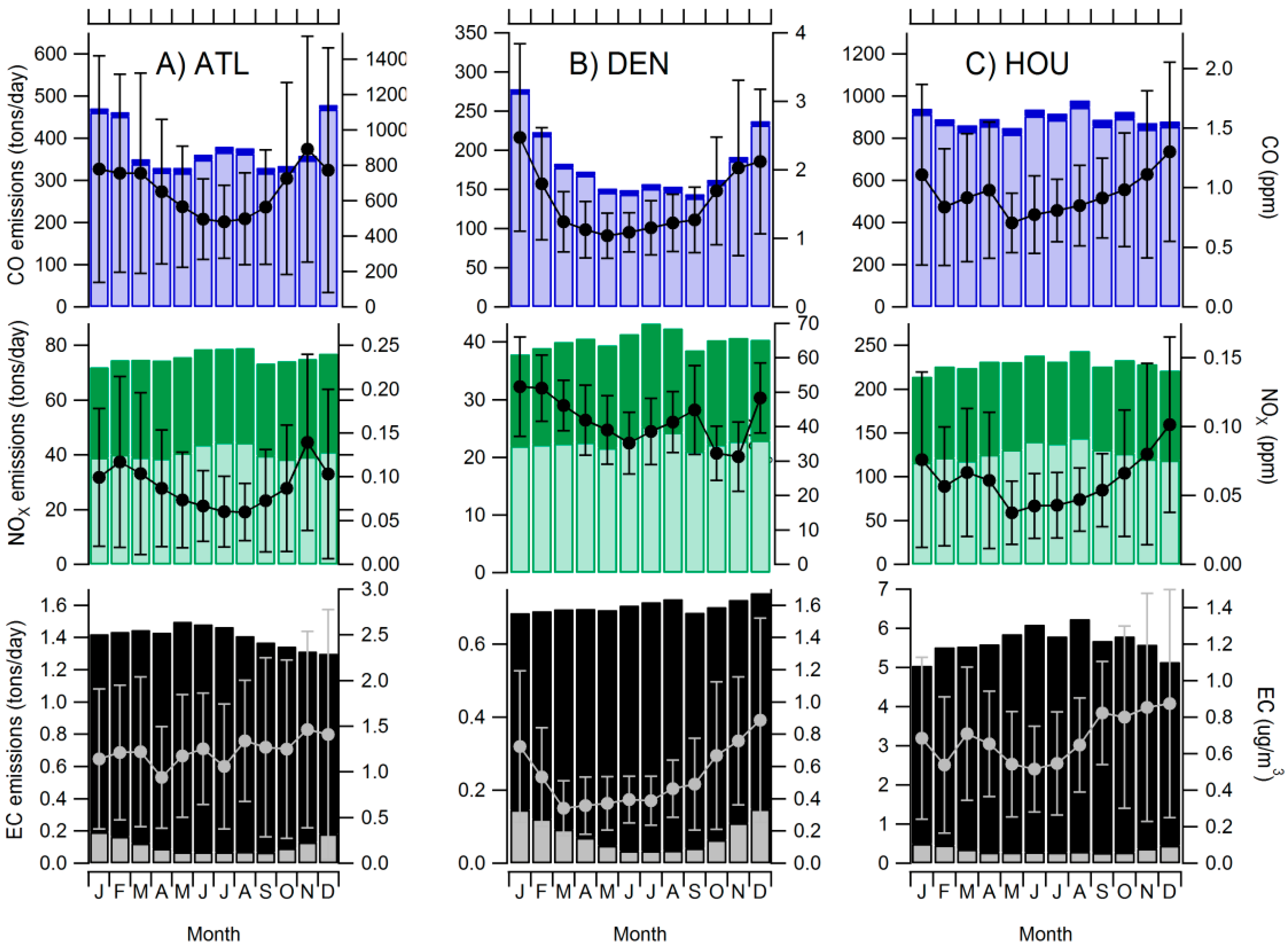
3.2.2. Emissions-Based Indicators

| Urban Area | Type of Mobile Source Pollution | EC | NOx | CO |
|---|---|---|---|---|
| Atlanta, GA | Diesel | 0.64 | 0.36 | * |
| Gasoline | * | 0.38 | 0.62 | |
| Combined | 0.32 | 0.36 | 0.32 | |
| Denver, CO | Diesel | 0.70 | 0.30 | * |
| Gasoline | * | 0.32 | 0.68 | |
| Combined | 0.33 | 0.29 | 0.37 | |
| Houston, TX | Diesel | 0.55 | 0.44 | * |
| Gasoline | * | 0.35 | 0.65 | |
| Combined | 0.22 | 0.38 | 0.40 |
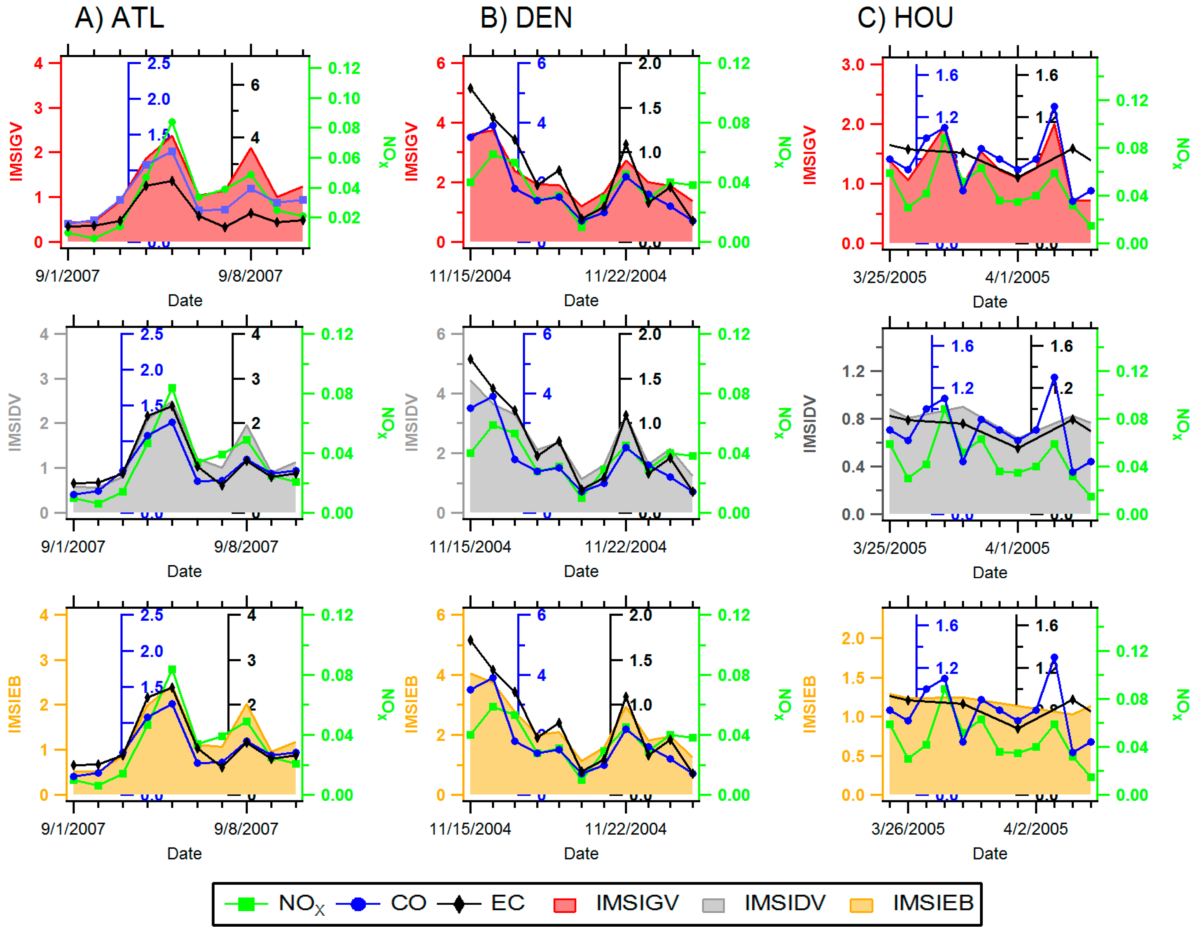
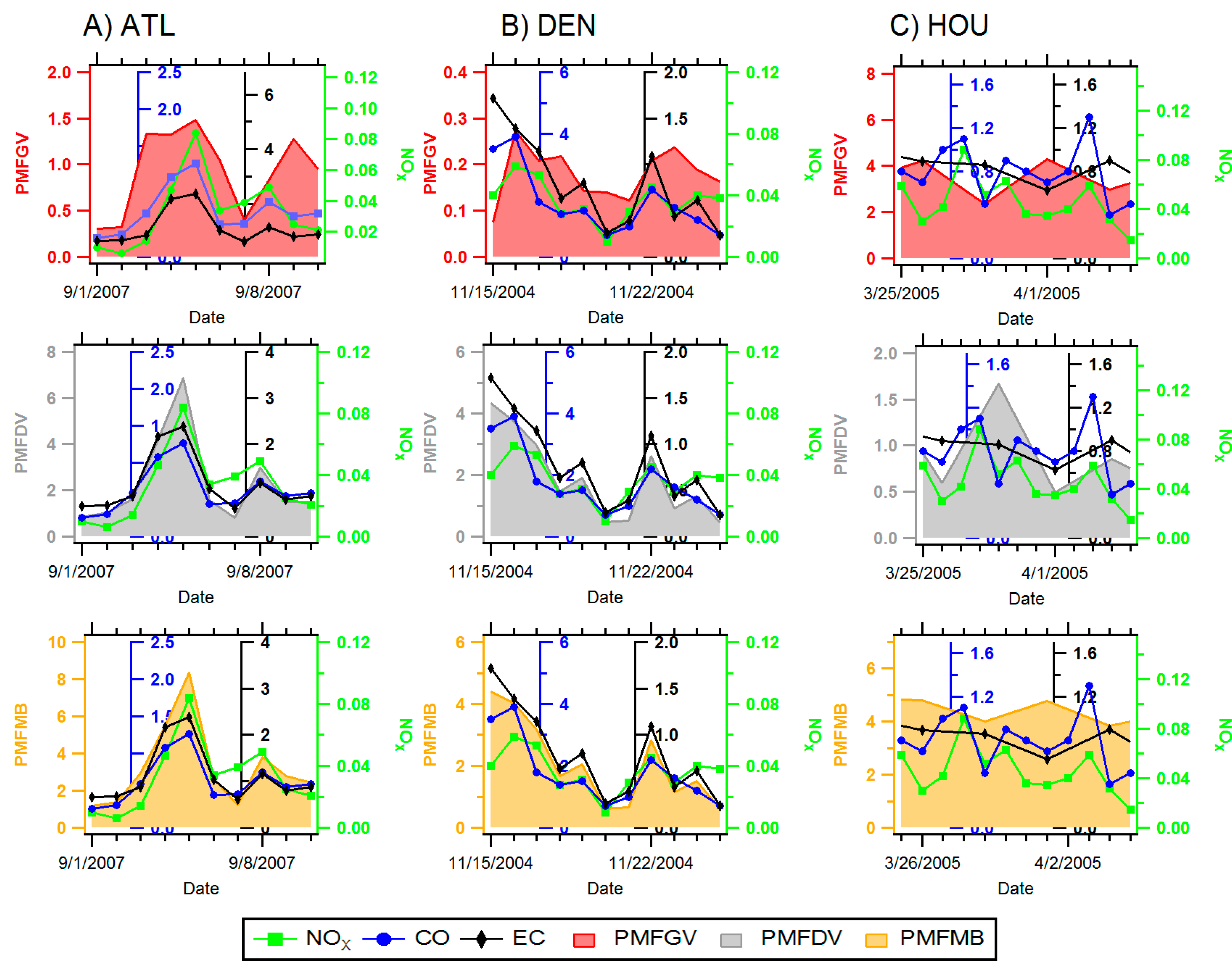
3.3. Temporal Analysis of Single Pollutant and Multipollutant Metrics

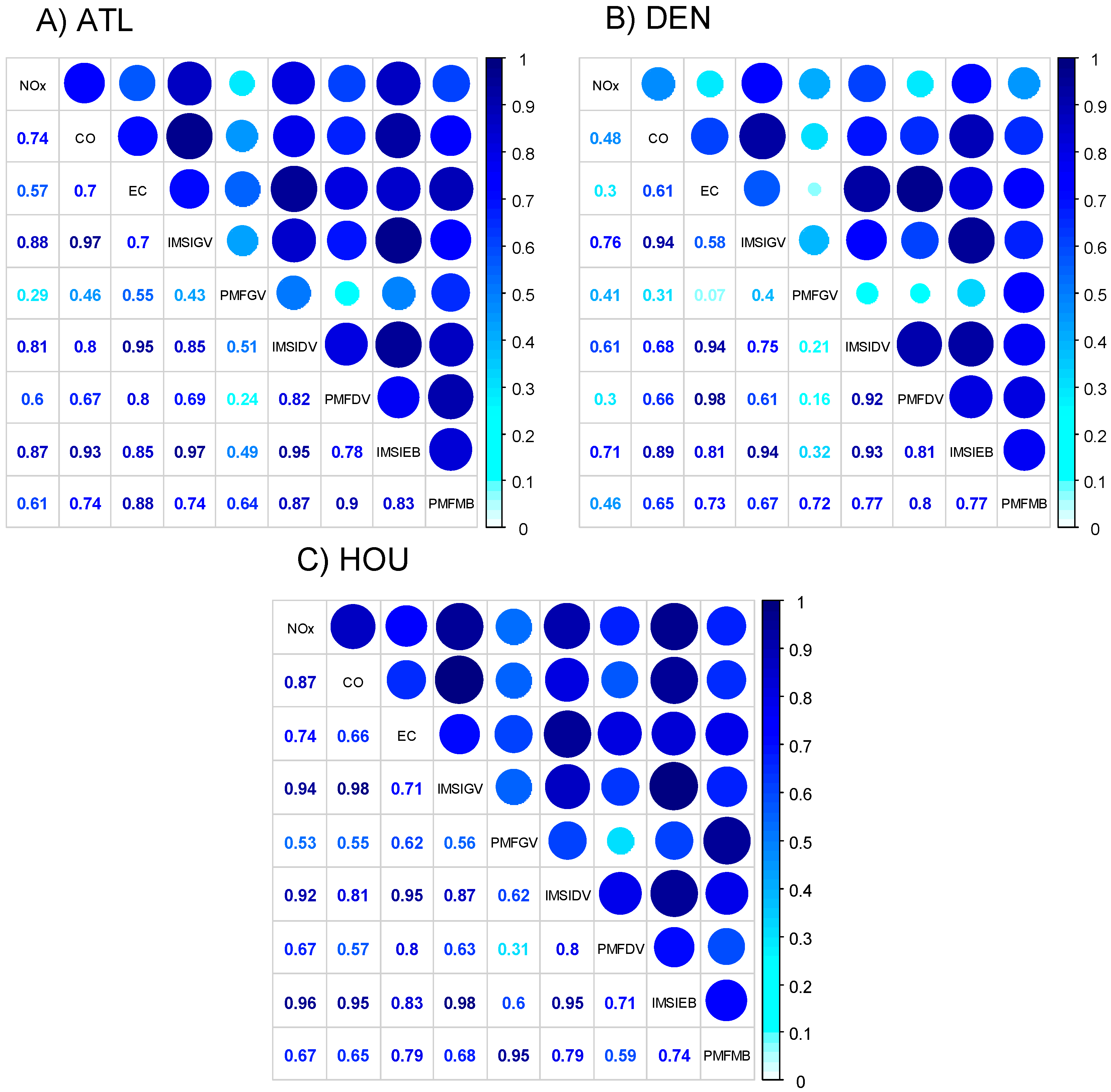
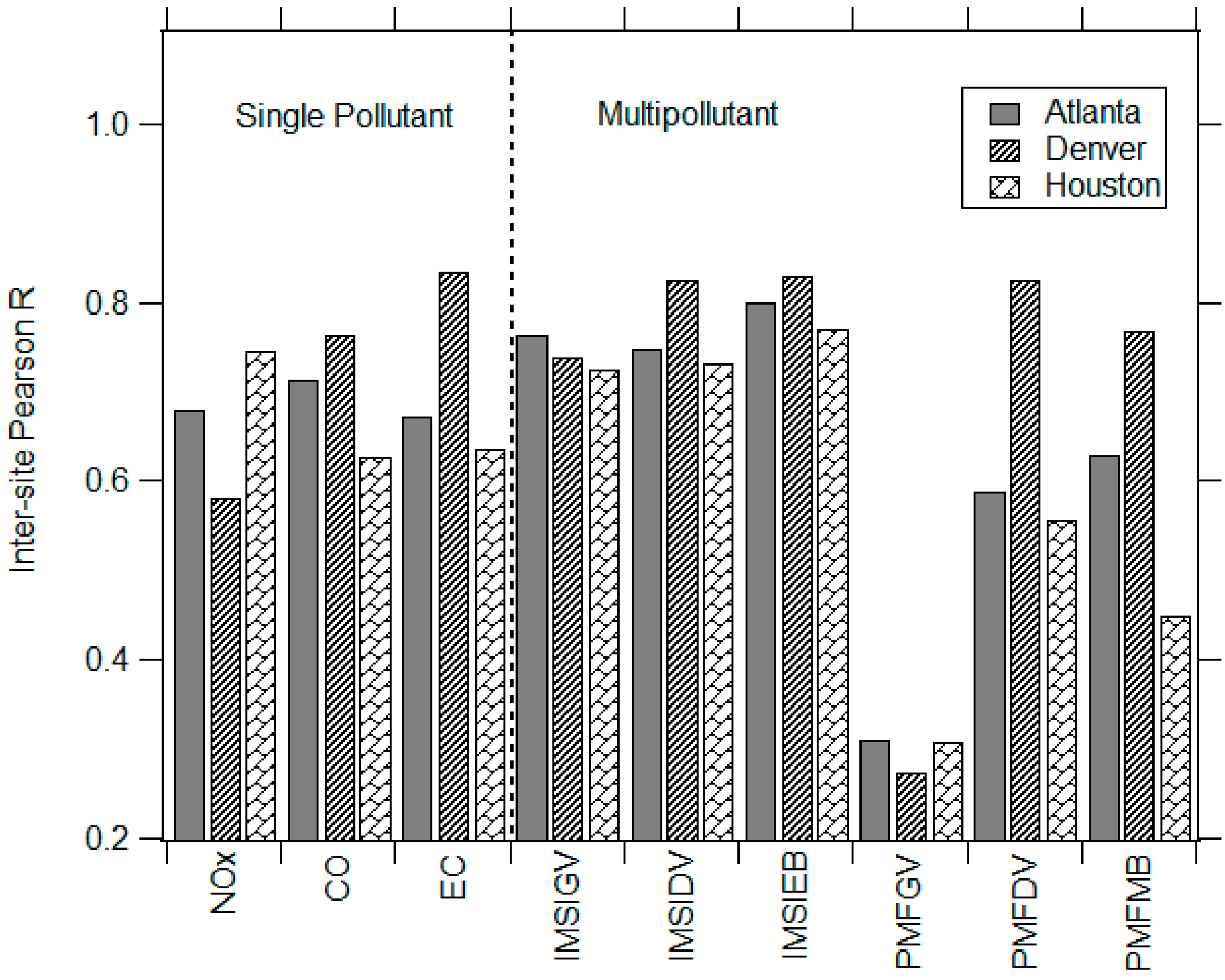
3.4. Inter-Site Spatial Comparisons of Metrics in Different Locations


4. Discussion
5. Conclusions and Future Work
Supplementary Files
Supplementary File 1Acknowledgments
Author Contributions
Conflicts of Interest
References
- Bell, M.L.; Peng, R.D.; Dominici, F.; Samet, J.M. Emergency hospital admissions for cardiovascular diseases and ambient levels of carbon monoxide: Results for 126 United States urban counties, 1999–2005. Circulation 2009, 120, 949–955. [Google Scholar] [PubMed]
- Folinsbee, L.J. Does nitrogen dioxide exposure increase airways responsiveness? Toxicol. Ind. Health 1992, 8, 273–283. [Google Scholar]
- Hoek, G.; Raaschou-Nielsen, O. Impact of fine particles in ambient air on lung cancer. Chin. J. Cancer 2014, 33, 197–203. [Google Scholar] [PubMed]
- Samoli, E.; Peng, R.; Ramsay, T.; Pipikou, M.; Touloumi, G.; Dominici, F.; Burnett, R.; Cohen, A.; Krewski, D.; Samet, J. Acute effects of ambient particulate matter on mortality in Europe and North America: Results from the APHENA study. Environ. Health Perspect. 2008, 116, 1480–1486. [Google Scholar] [CrossRef] [PubMed]
- U.S. EPA. Integrated Science Assessment for Particulate Matter (Second External Review Draft); Research Triangle Park: Triangle Park, NC, USA, 2009.
- U.S. EPA. Integrated Science Assessment for Oxides of Nitrogen—Health Criteria; Research Triangle Park: Triangle Park, NC, USA, 2008.
- Dominici, F.; Peng, R.D.; Barr, C.D.; Bell, M.L. Protecting human health from air pollution: Shifting from a single-pollutant to a multipollutant approach. Epidemiology 2010, 21, 187–194. [Google Scholar] [CrossRef] [PubMed]
- Hidy, G.M.; Pennell, W.T. Multipollutant air quality management. J. Air Waste Manage. Assoc. 2010, 60, 645–674. [Google Scholar] [CrossRef]
- Johns, D.O.; Stanek, L.W.; Walker, K.; Benromdhane, S.; Hubbell, B.; Ross, M.; Devlin, R.B.; Costa, D.L.; Greenbaum, D.S. Practical advancement of multipollutant scientific and risk assessment approaches for ambient air pollution. Environ. Health Perspect. 2012, 120, 1238–1242. [Google Scholar] [CrossRef] [PubMed]
- Mauderly, J.L.; Burnett, R.T.; Castillejos, M.; Ozkaynak, H.; Samet, J.M.; Stieb, D.M.; Vedal, S.; Wyzga, R.E. Is the air pollution health research community prepared to support a multipollutant air quality management framework? Inhal. Toxicol. 2010, 22, 1–19. [Google Scholar]
- Oakes, M.; Baxter, L.; Long, T.C. Evaluating the application of multipollutant exposure metrics in air pollution health studies. Environ. Int. 2014, 69C, 90–99. [Google Scholar] [CrossRef] [PubMed]
- HEI Panel on the Health Effects of Traffic-Related Air Pollution. Traffic-Related Air Pollution: A Critical Review of the Literature on Emissions, Exposure and Health Effects; HEI: Boston, MA, USA, 2010. [Google Scholar]
- U.S. EPA. Integrated Science Assessment for Carbon Monoxide (Final Report); U.S. EPA: Washington, DC, USA, 2010.
- Dallmann, T.R.; Kirchstetter, T.W.; Demartini, S.J.; Harley, R.A. Quantifying on-road emissions from gasoline-powered motor vehicles: Accounting for the presence of medium- and heavy-duty diesel trucks. Environ. Sci. Technol. 2013, 47, 13873–13881. [Google Scholar] [CrossRef] [PubMed]
- Paatero, P. Least squares formulation of robust non-negative factor analysis. Chemom. Intell. Lab. Syst. 1997, 37, 23–35. [Google Scholar] [CrossRef]
- Paatero, P.; Tapper, U. Positive matrix factorization—A nonnegative factor model with optimal utilization of error-estimates of data values. Environmetrics 1994, 5, 111–126. [Google Scholar] [CrossRef]
- Thurston, G.D.; Ito, K.; Mar, T.; Christensen, W.F.; Eatough, D.J.; Henry, R.C.; Kim, E.; Laden, F.; Lall, R.; Larson, T.V.; et al. Workgroup report: Workshop on source apportionment of particulate matter health effects—Intercomparison of results and implications. Environ. Health Perspect. 2005, 113, 1768–1774. [Google Scholar] [CrossRef]
- Watson, J.G.; Cooper, J.A.; Huntzicker, J.J. The effective variance weighting for least-squares calculations applied to the mass balance receptor model. Atmos. Environ. 1984, 18, 1347–1355. [Google Scholar] [CrossRef]
- Hopke, P.K.; Ito, K.; Mar, T.; Christensen, W.F.; Eatough, D.J.; Henry, R.C.; Kim, E.; Laden, F.; Lall, R.; Larson, T.V.; et al. PM source apportionment and health effects: 1. Intercomparison of source apportionment results. J. Expo. Sci. Environ. Epidemiol. 2006, 16, 275–286. [Google Scholar] [CrossRef]
- Sarnat, J.A.; Marmur, A.; Klein, M.; Kim, E.; Russell, A.G.; Sarnat, S.E.; Mulholland, J.A.; Hopke, P.K.; Tolbert, P.E. Fine particle sources and cardiorespiratory morbidity: An application of chemical mass balance and factor analytical source-apportionment methods. Environ. Health Perspect. 2008, 116, 459–466. [Google Scholar] [PubMed]
- Pachon, J.E.; Balachandran, S.; Hu, Y.; Mulholland, J.A.; Darrow, L.A.; Sarnat, J.A.; Tolbert, P.E.; Russell, A.G. Development of outcome-based, multipollutant mobile source indicators. J. Air Waste Manage. Assoc. 2012, 62, 431–442. [Google Scholar] [CrossRef]
- The 2008 National Emissions Inventory. Available online: http://www.epa.gov/ttnchie1/net/2008inventory.html (accessed on 13 November 2014).
- Hansen, D.A.; Edgerton, E.S.; Hartsell, B.E.; Jansen, J.J.; Kandasamy, N.; Hidy, G.M.; Blanchard, C.L. The southeastern aerosol research and characterization study: Part I—Overview. J. Air Waste Manage. Assoc. 2003, 53, 1460–1471. [Google Scholar] [CrossRef]
- Vedal, S.; Hannigan, M.P.; Dutton, S.J.; Miller, S.L.; Milford, J.B.; Rabinovitch, N.; Kim, S.Y.; Sheppard, L. The Denver Aerosol Sources and Health (DASH) study: Overview and early findings. Atmos. Environ. 2009, 43, 1666–1673. [Google Scholar] [CrossRef]
- Technology Transfer Network (TTN) Air Quality System. Available online: http://www.epa.gov/ttn/airs/airsaqs/detaildata/downloadaqsdata.htm (accessed on 13 November 2014).
- Atmospheric, Research & Analysis, Inc. Available online: http://www.atmospheric-research.com (accessed on 13 November 2014).
- Dutton, S.J.; Schauer, J.J.; Vedal, S.; Hannigan, M.P. PM2.5 characterization for time series studies: Pointwise uncertainty estimation and bulk speciation methods applied in Denver. Atmos. Environ. 2009, 43, 1136–1146. [Google Scholar] [CrossRef]
- Dutton, S.J.; Williams, D.E.; Garcia, J.K.; Vedal, S.; Hannigan, M.P. PM2.5 characterization for time series studies: Organic molecular marker speciation methods and observations from daily measurements in Denver. Atmos. Environ. 2009, 43, 2018–2030. [Google Scholar] [CrossRef]
- Allred, E.N.; Bleecker, E.R.; Chaitman, B.R.; Dahms, T.E.; Gottlieb, S.O.; Hackney, J.D.; Pagano, M.; Selvester, R.H.; Walden, S.M.; Warren, J. Short-term effects of carbon monoxide exposure on the exercise performance of subjects with coronary artery disease. N. Engl. J. Med. 1989, 321, 1426–1432. [Google Scholar] [CrossRef] [PubMed]
- EPA Positive Matrix Factorization (PMF) Model. Available online: http://www.epa.gov/heasd/research/pmf.html (accessed on 13 November 2014).
- Balachandran, S.; Chang, H.H.; Pachon, J.E.; Holmes, H.A.; Mulholland, J.A.; Russell, A.G. Bayesian-based ensemble source apportionment of PM2.5. Environ. Sci. Technol. 2013, 47, 13511–13518. [Google Scholar] [CrossRef] [PubMed]
- Xie, M.; Hannigan, M.P.; Dutton, S.J.; Milford, J.B.; Hemann, J.G.; Miller, S.L.; Schauer, J.J.; Peel, J.L.; Vedal, S. Positive matrix factorization of PM(2.5): Comparison and implications of using different speciation data sets. Environ. Sci. Technol. 2012, 46, 11962–11970. [Google Scholar] [CrossRef] [PubMed]
- Baxter, L.K.; Duvall, R.M.; Sacks, J. Examining the effects of air pollution composition on within region differences in PM2.5 mortality risk estimates. J. Expo. Sci. Environ. Epidemiol. 2013, 23, 457–465. [Google Scholar] [CrossRef] [PubMed]
- Kim, E.; Hopke, P.K. Comparison between sample-species specific uncertainties and estimated uncertainties for the source apportionment of the speciation trends network data. Atmos. Environ. 2007, 41, 567–575. [Google Scholar] [CrossRef]
- Lee, D.; Balachandran, S.; Pachon, J.; Shankaran, R.; Lee, S.; Mulholland, J.A.; Russell, A.G. Ensemble-trained PM2.5 source apportionment approach for health studies. Environ. Sci. Technol. 2009, 43, 7023–7031. [Google Scholar] [CrossRef] [PubMed]
- Marmur, A.; Park, S.K.; Mulholland, J.A.; Tolbert, P.E.; Russell, A.G. Source apportionment of PM2.5 in the southeastern United States using receptor and emissions-based models: Conceptual differences and implications for time-series health studies. Atmos. Environ. 2006, 40, 2533–2551. [Google Scholar] [CrossRef]
- Hasheminassab, S.; Daher, N.; Ostro, B.D.; Sioutas, C. Long-term source apportionment of ambient fine particulate matter (PM2.5) in the Los Angeles Basin: A focus on emissions reduction from vehicular sources. Environ. Pollut. 2014, 193, 54–64. [Google Scholar] [CrossRef] [PubMed]
- Xie, M.; Barsanti, K.C.; Hannigan, M.P.; Dutton, S.J.; Vedal, S. Positive matrix factorization of PM2.5—Eliminating the effects of gas/particle partitioning of semivolatile organic compounds. Atmos. Chem. Phys. 2013, 13, 7381–7393. [Google Scholar] [CrossRef]
- Xie, M.; Hannigan, M.P.; Barsanti, K.C. Impact of gas/particle partitioning of semi-volatile organic compounds on source apportionment with postive matrix factorization. Environ. Sci. Technol. 2014, 48, 9053–9060. [Google Scholar] [CrossRef] [PubMed]
- Kioumourtzoglou, M.-A.; Coull, B.A.; Dominici, F.; Koutrakis, P.; Schwartz, J.D.; Suh, H. The impact of source contribution uncertainty on the effects of source-specific PM2.5 on hospital admissions: A case study in Boston, MA. J. Expo. Sci. Environ. Epidemiol. 2014, 24, 365–371. [Google Scholar] [CrossRef] [PubMed]
- Dionisio, K.L.; Baxter, L.K.; Chang, H.H. An empirical assessment of exposure measurement error and effect attenuation in bipollutant epidemiologic models. Environ. Health Perspect. 2014, 122, 1216–1224. [Google Scholar] [PubMed]
- Goldman, G.T.; Mulholland, J.A.; Russell, A.G.; Srivastava, A.; Strickland, M.J.; Klein, M.; Waller, L.A.; Tolbert, P.E.; Edgerton, E.S. Ambient air pollutant measurement error: Characterization and impacts in a time-series epidemiologic study in Atlanta. Environ. Sci. Technol. 2010, 44, 7692–7698. [Google Scholar] [CrossRef] [PubMed]
© 2014 by the authors; licensee MDPI, Basel, Switzerland. This article is an open access article distributed under the terms and conditions of the Creative Commons Attribution license (http://creativecommons.org/licenses/by/4.0/).
Share and Cite
Oakes, M.M.; Baxter, L.K.; Duvall, R.M.; Madden, M.; Xie, M.; Hannigan, M.P.; Peel, J.L.; Pachon, J.E.; Balachandran, S.; Russell, A.; et al. Comparing Multipollutant Emissions-Based Mobile Source Indicators to Other Single Pollutant and Multipollutant Indicators in Different Urban Areas. Int. J. Environ. Res. Public Health 2014, 11, 11727-11752. https://doi.org/10.3390/ijerph111111727
Oakes MM, Baxter LK, Duvall RM, Madden M, Xie M, Hannigan MP, Peel JL, Pachon JE, Balachandran S, Russell A, et al. Comparing Multipollutant Emissions-Based Mobile Source Indicators to Other Single Pollutant and Multipollutant Indicators in Different Urban Areas. International Journal of Environmental Research and Public Health. 2014; 11(11):11727-11752. https://doi.org/10.3390/ijerph111111727
Chicago/Turabian StyleOakes, Michelle M., Lisa K. Baxter, Rachelle M. Duvall, Meagan Madden, Mingjie Xie, Michael P. Hannigan, Jennifer L. Peel, Jorge E. Pachon, Siv Balachandran, Armistead Russell, and et al. 2014. "Comparing Multipollutant Emissions-Based Mobile Source Indicators to Other Single Pollutant and Multipollutant Indicators in Different Urban Areas" International Journal of Environmental Research and Public Health 11, no. 11: 11727-11752. https://doi.org/10.3390/ijerph111111727