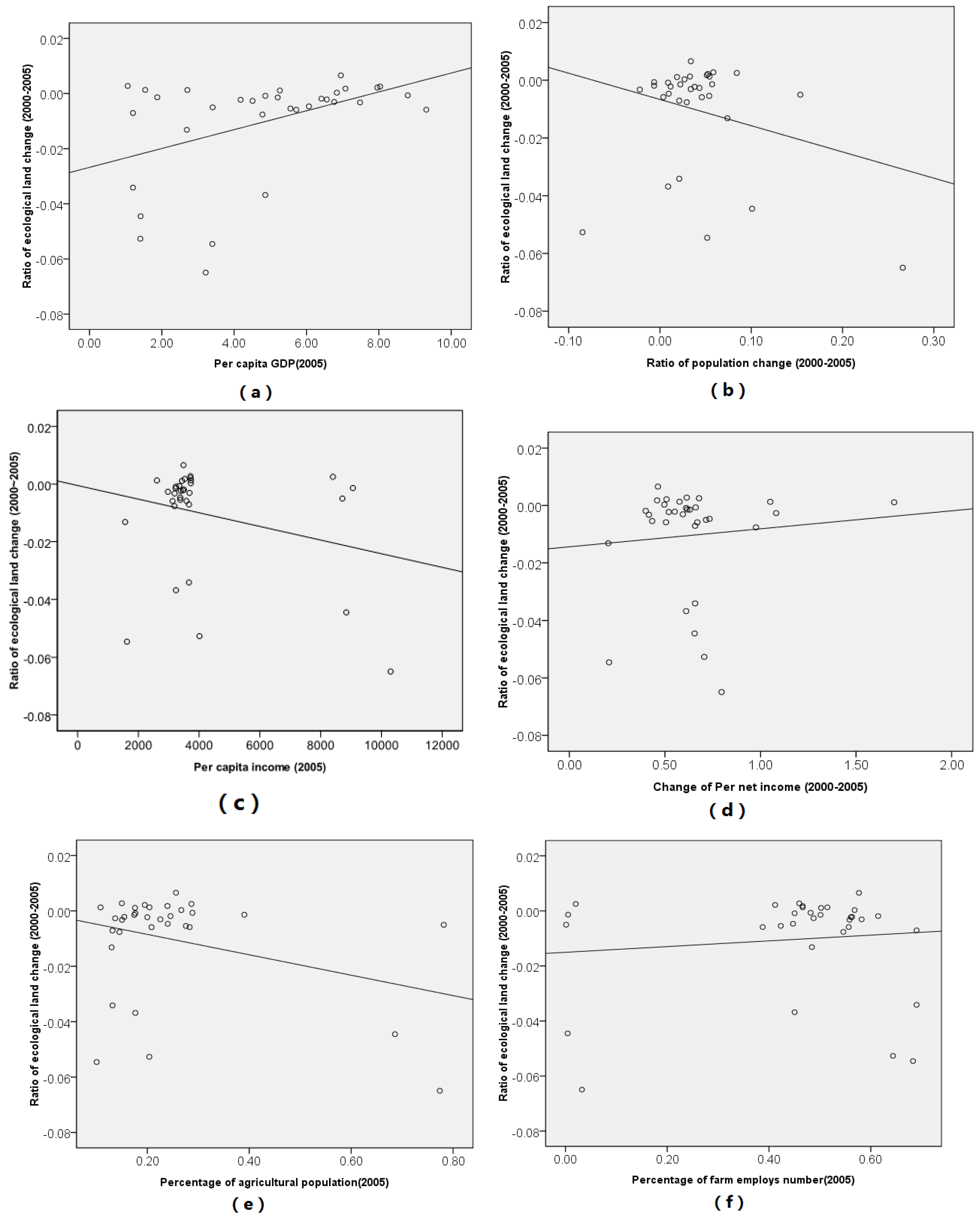
3.2.1. Local Moran’s Ii
To explore in depth the local spatial disparities of ecological land change from 1990 to 2005 in the Poyang Lake Eco-economic Zone, we used the OpenGeoda software package and obtained the results of the local Moran’s I and its significant test during the 1990 to 2000, 2000 to 2005, and 1990 to 2005 time periods (see
Table 3).
Table 3 presents the range of local Moran’s I values from 1990 to 2005 of each county in the Poyang Lake Eco-economic Zone (−0.5106, 1.3989). The negative value of the local Moran's I imply that there is spatial heterogeneity in the ecological land. The range of local Moran’s I values of each county in the study area is 1.8825 during the 1990 to 2000 time period. The maximum value of the local Moran’s I is 1.2356 during the 2000 to 2005 time period and 1.3989 during the 1990 to 2005 time period, and all the maximum values are from Nanchang County. The minimum value of the local Moran’s I is −0.8155 during the 1990 to 2000 and is located in Jingdezhen County. The minimum value of the local Moran’s I during the 2000 to 2005 time period is located in Jinxian County.
Table 3 also indicates that 12% of the counties during the 1990 to 2000 time period and 19% of the counties during the 2000 to 2005 time period are significantly heterogeneous. The changes in the rate of local Moran’s I values indicate the upward and downward trends, respectively.
Table 3 also indicates that the spatial clustering of ecological land change at the county level weakened and the spatial heterogeneity increased.
Table 1.
Ecological land changes in the Poyang Lake Eco-economic Zone from 1990 to 2005.
Table 1.
Ecological land changes in the Poyang Lake Eco-economic Zone from 1990 to 2005.
| Ecological Land Type | 1990 | 2000 | 2005 |
|---|
| Area (km2) | Percentage (%) | Area (km2) | Percentage (%) | Area (km2) | Percentage (%) |
|---|
| Forestland | 22,044.98 | 72.17 | 22,056.81 | 72.25 | 22,040.23 | 72.58 |
| Grassland | 2,182.70 | 7.15 | 2,165.48 | 7.09 | 2,127.52 | 7.01 |
| Wetland | 6,318.69 | 20.69 | 6,306.43 | 20.66 | 6,200.45 | 20.42 |
| Ecological land | 30,546.37 | 100.00 | 30,528.72 | 100.00 | 30,368.20 | 100.00 |
Table 2.
Global Moran’s I value and its statistical test for ecological land change from 1990 to 2005.
Table 2.
Global Moran’s I value and its statistical test for ecological land change from 1990 to 2005.
| Time period | Moran’s
I | E(I) | Mean | ZScore |
|---|
| 1990~2000 | 0.2091 * | −0.0323 | 0.0298 | 2.2269 |
| 2000~2005 | 0.1380 * | −0.0323 | −0.0299 | 1.9848 |
| 1990~2005 | 0.1646 * | −0.0323 | −0.0302 | 2.0425 |
Table 3.
Related parameters of the local Moran’s I for ecological land change in the Poyang Lake Eco-economic Zone from 1990 to 2005.
Table 3.
Related parameters of the local Moran’s I for ecological land change in the Poyang Lake Eco-economic Zone from 1990 to 2005.
| Time period | Minimum | Maximum | Mean | Moran’s Ii (+) | Moran’s Ii(−) | Range |
|---|
| 1990~2000 | −0.8155 | 1.0670 | 0.2025 | 9.2379 | 2.7569 | 1.8825 |
| 2000~2005 | −0.4629 | 1.2356 | 0.1144 | 5.5991 | 1.9398 | 1.6985 |
| 1990~2005 | −0.5106 | 1.3989 | 0.5943 | 7.4170 | 2.3153 | 1.9095 |
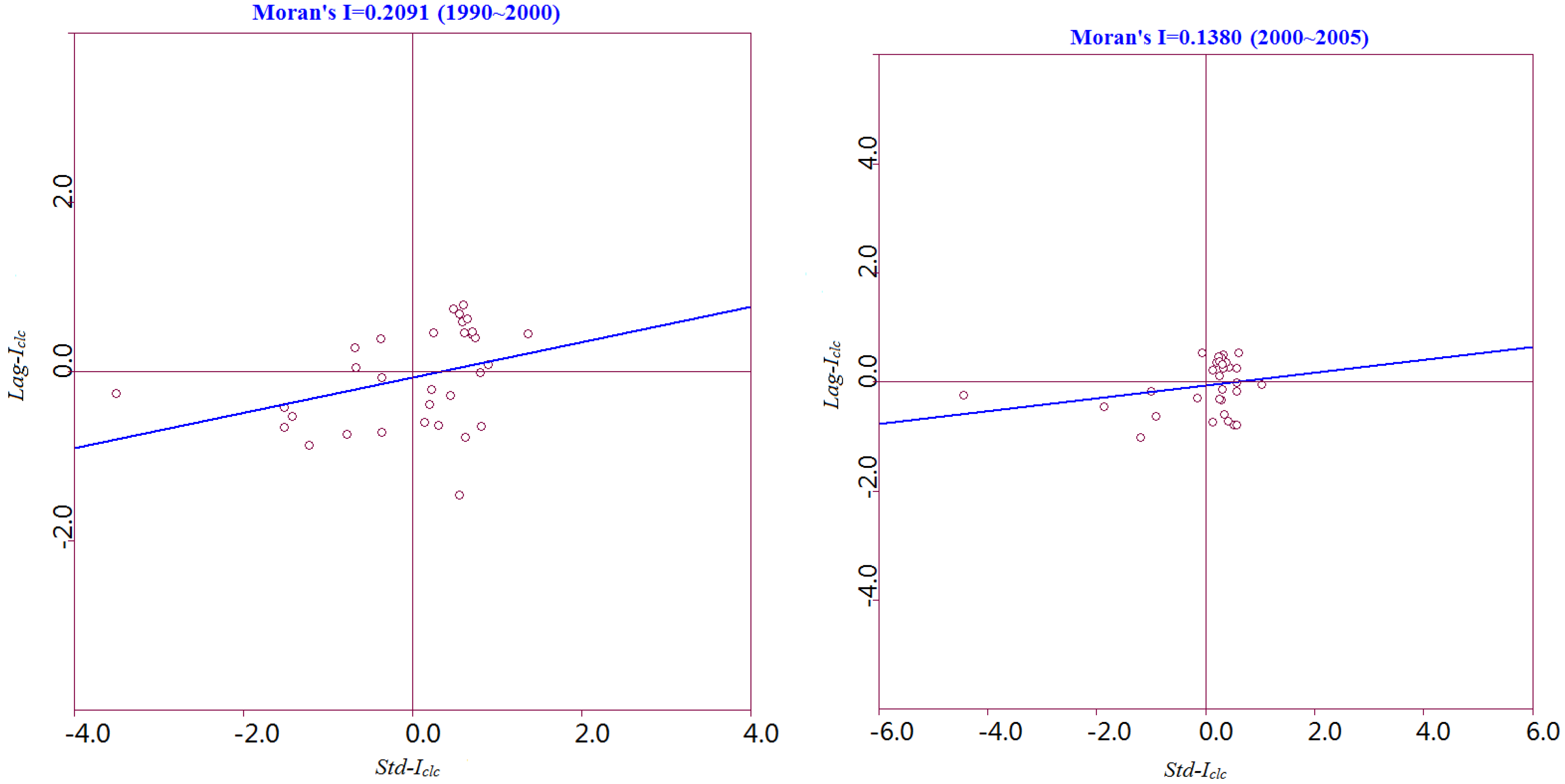
3.2.2. Spatial Association and Distribution Features Based on the Local Moran’s Ii
If the variable
Z and spatial variable
Wz at the research unit are calculated and used as the lateral axis and longitudinal axis, we can obtain the Moran scatter plot of ecological land change. Thus, the standardized value (Std-I
clc) of the research observations is used as the lateral axis, and the spatial lag value (Lag-I
clc) is the longitudinal axis. The Moran scatter plot of ecological land change composed of the local Moran's
Ii for each county in the Poyang Lake Eco-economic Zone is shown in
Figure 2.
A positive Std-I
clc value indicates that the research unit belongs to those areas that have high values of ecological land changes. A negative Std-I
clc belongs to those areas that have low values of ecological land change. The number of areas with a positive Std-I
clc value accounts for 72% of the land area during 1990 to 2005 (see
Table 4). The positive Lag-I
clc value in the Moran scatter plot indicates that the surrounding areas of research unit belong to those areas with high values of ecological land change. From
Table 4, we can see that the number of areas with a positive Lag-I
clc value account for 40% during 1990 to 2005. The number of areas with a positive Lag-I
clc value increased from 44% during 1990 to 2000 to 84% during 2000 to 2005, which implies that number of surrounding areas of research units with a high value of ecological land change increased because of the spatial association. The number of areas with a positive Std-I
clc value increased from 31% during 1990 to 2000 to 38% during 2000 to 2005.
Figure 2.
Moran scatter plot of the ecological land at the county level from 1990 to 2005. (Please provide figures with higher resolution.)
Figure 2.
Moran scatter plot of the ecological land at the county level from 1990 to 2005. (Please provide figures with higher resolution.)
Table 4.
Related parameters and disparity type of the standardized variable Z for ecological land change at the county level (%).
Table 4.
Related parameters and disparity type of the standardized variable Z for ecological land change at the county level (%).
| Time period | Std-Iclc >0 | Std-Iclc <0 | Lag-Iclc >0 | Lag-Iclc <0 | H–H | L–L | L–L | H–L |
|---|
| Ratio | Ratio | Ratio | Ratio | Comparison ratio | Ratio | Comparison ratio | Ratio | Comparison ratio | Ratio | Comparison ratio | Ratio |
|---|
| 1990~2000 | 68.75 | 31.25 | 43.75 | 56.25 | S+L+ | 34.38 | S+L− | 34.38 | S−L− | 21.88 | S−L+ | 9.38 |
| 2000~2005 | 62.50 | 37.50 | 84.38 | 15.63 | S+L+ | 59.38 | S+L− | 3.13 | S−L− | 25.00 | S−L+ | 12.50 |
| 1990~2005 | 71.88 | 28.13 | 40.63 | 59.38 | S+L+ | 37.50 | S+L− | 34.38 | S−L− | 25.00 | S−L+ | 3.13 |
Using to the positive or negative attributes of the Std-I
clc and Lag-I
clc values, we can obtain the four types of areas of ecological land change (
Table 4). The four types of areas are referred to as the High-High (H-H) type, which has a positive correlation; the Low-Low (L-L) type, which has a positive correlation; the Low-High (L-H) type, which has a negative correlation; and the High-Low (H-L) type, which has a negative correlation.
From
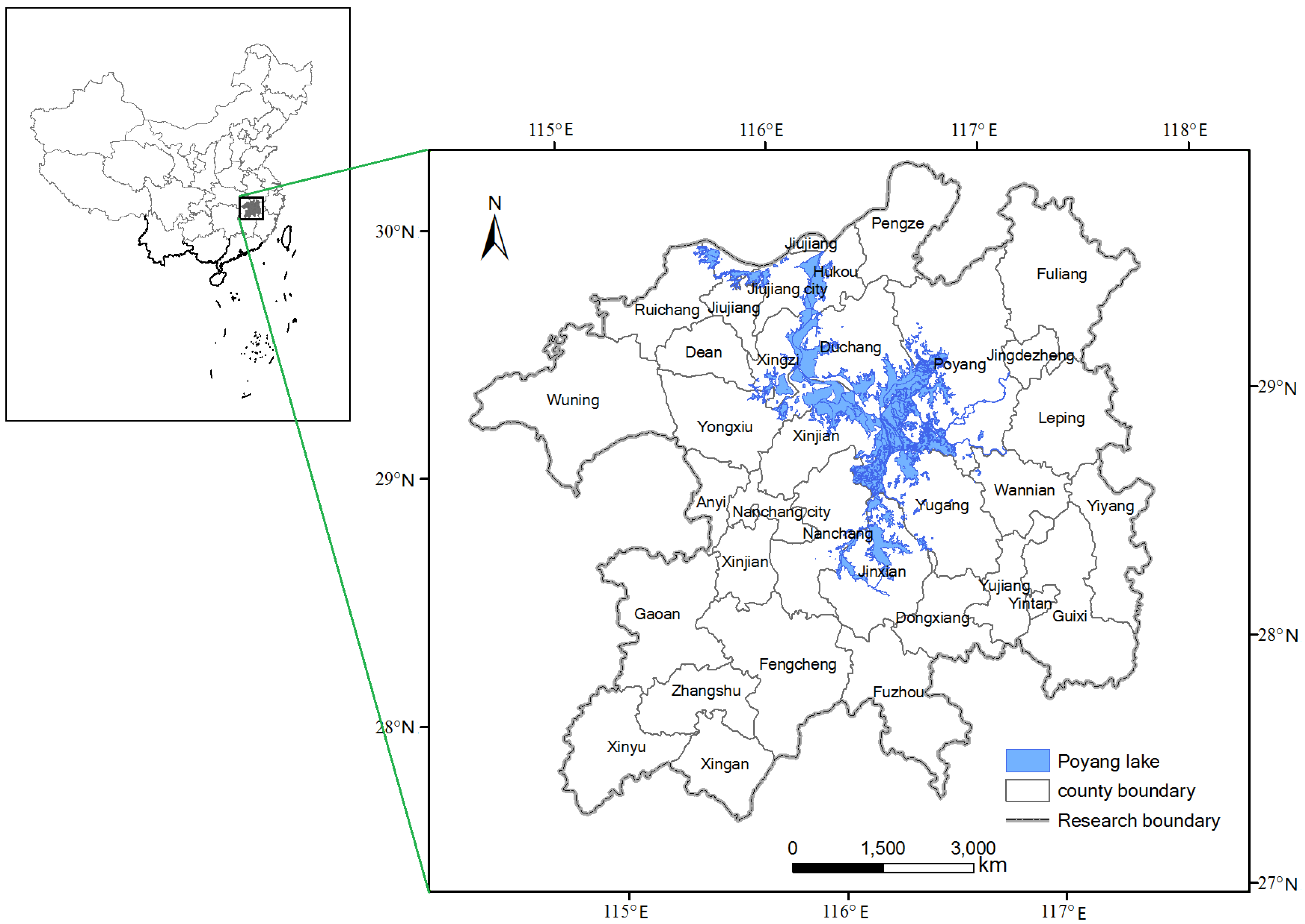
Table 4, we can conclude that the number of areas that belong to the L-L type accounted for 30% during 1990 to 2005 (e.g., the counties of Yugang, Pengze, and Fuliang). This result occurred primarily because of the low urbanization and industrialization in the aforementioned areas. From
Table 4, we can see that the number of the areas that belong to the H-H type accounted for 34% during 1990 to 2005, (e.g., Jiujiang, Fuzhoushi, and Xinyushi countie). This result occurred because of the greater urbanization and industrialization level in the aforementioned areas.
To effectively explore the spatial characteristics of ecological land change in the Poyang Lake Eco-economic Zone during 1990 to 2005, LISA clustering maps of two time stages formed by matching the type to which the area belongs with the corresponding spatial location of each county during 1990 to 2000 and during 2000 to 2005 are shown in
Figure 3 and
Figure 4.
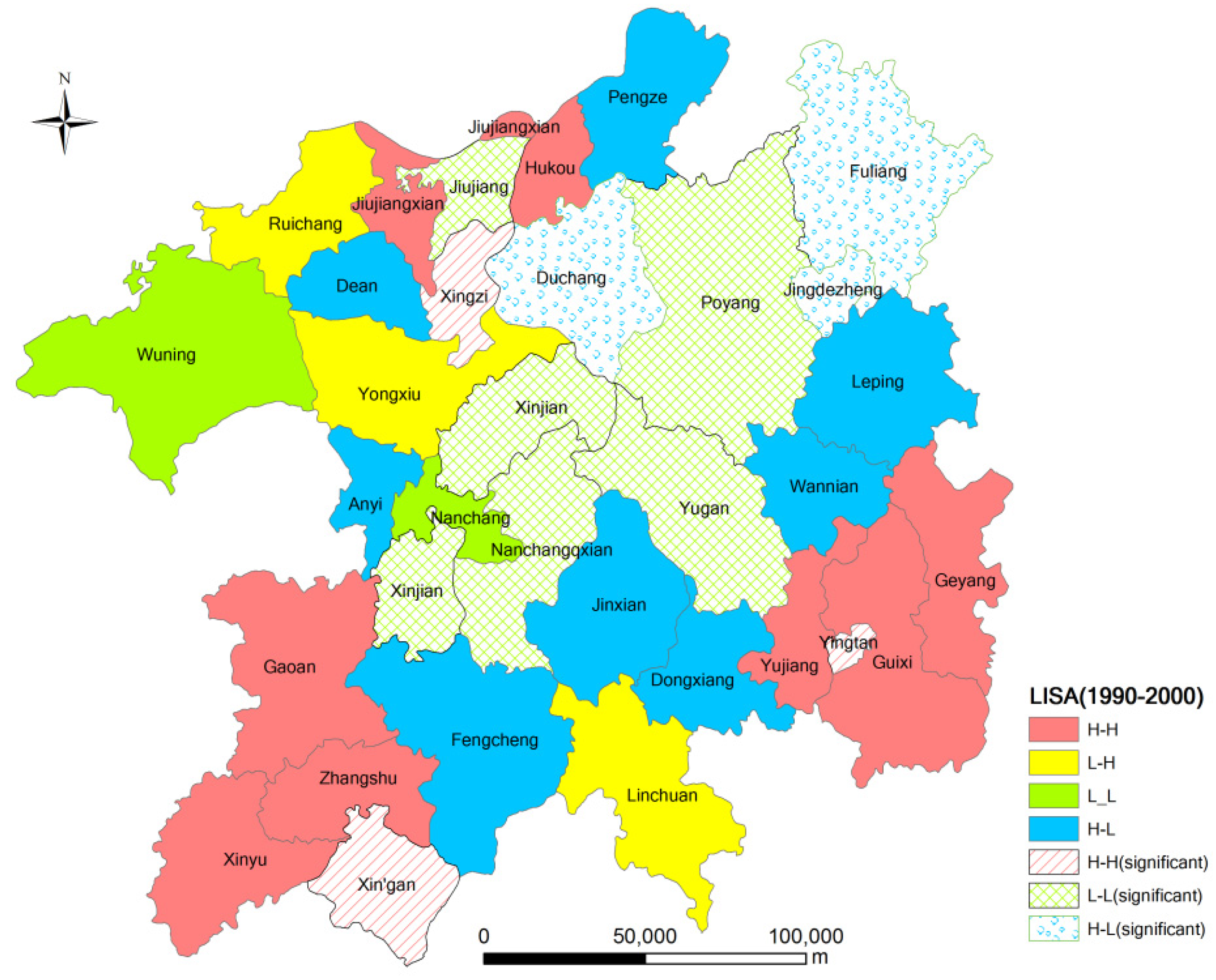
Figure 3.
LISA clustering of ecological land change in the Poyang Lake Eco-economic Zone during 1990-2000 at the county level.
Figure 3.
LISA clustering of ecological land change in the Poyang Lake Eco-economic Zone during 1990-2000 at the county level.
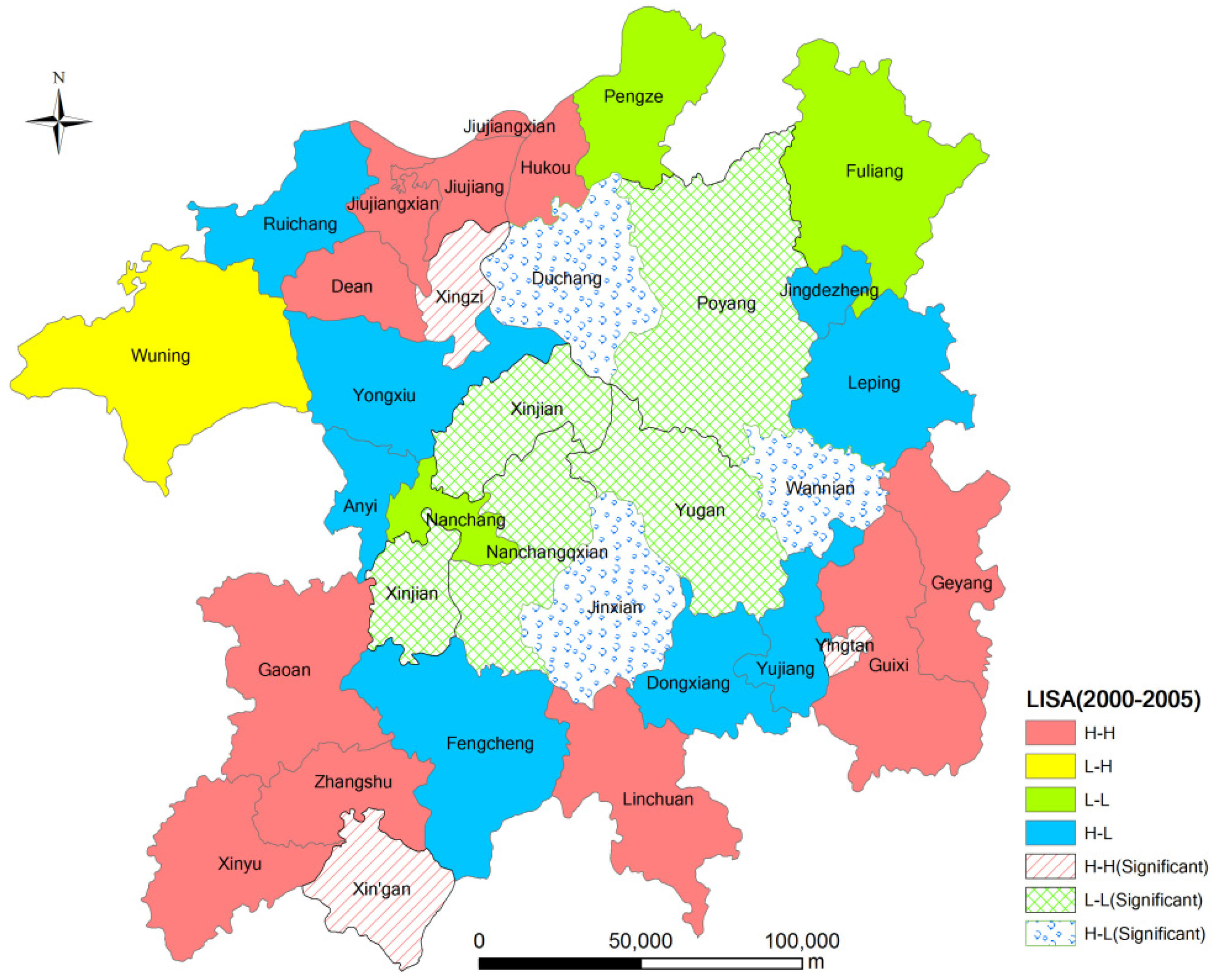
Figure 3 and
Figure 4 indicate that the areas that belong to the H-H type have a positive spatial autocorrelation during 1990 to 2000 and during 2000 to 2005, where Std-I
clc > 0 and Lag-I
clc > 0. The local spatial disparities of ecological land change are stronger with local homogeneity in those areas, where high values are surrounded by neighbors with high values.
Table 4 indicates that the proportion of those type of areas increased from 34% during 1990 to 2000 to 59% during 2000 to 2005. Especially at the 5% significance level, the Xingan, Yingtan, and Xinzi counties have a significantly positive relationship for 1990 to 2000 and 2000 to 2005 (
Figure 3 and
Figure 4).
From
Figure 3 and
Figure 4, we can conclude that the areas that belong to the L-L type have a positive spatial autocorrelation, where Std-I
clc < 0 and Lag-I
clc < 0. This result implies that the local spatial disparities of ecological land change is small in those areas, and low values are surrounded by neighbors with low values. The number of L-L-type areas increased from 7 during 1990 to 2000 to 8 during 2000 to 2005. The L-L type area ratio (22%) is less than the average level in the Poyang Lake Eco-economic Zone during 1999 to 2000. All areas that belong to this type are significantly distributed in the surrounding areas of the Poyang Lake, where protection policies of ecological land have been effective in the past 15 years. At the 5% significance level, Poyang and Yugang Counties both have significantly positive relationships during 1990 to 2005 and during 2000 to 2005 (
Figure 3 and
Figure 4).
Figure 4.
LISA clustering of ecological land change in the Poyang Lake Eco-economic Zone during 2000–2005 at the county level.
Figure 4.
LISA clustering of ecological land change in the Poyang Lake Eco-economic Zone during 2000–2005 at the county level.
The areas that belong to the H-L type exhibit a negative spatial autocorrelation, where Std-I
clc > 0 and Lag-I
clc < 0. This result implies that clusters of dissimilar values (e.g., locations with high values surrounded by neighbors with low values) forms the hot spots of local heterogeneity. There are three areas that belonged to the H-L type during 1990 to 2000 and four areas that belonged during 2000 to 2005. At the 5% significance level, Duchang and Fuliang Counties have significantly negative relationships during 1990 to 2005 (
Figure 3).
The areas that belong to the L-H type have a negative spatial autocorrelation, where Std-I
clc < 0 and Lag-I
clc > 0 (
Figure 3 and
Figure 4). This result implies that clusters of dissimilar values (e.g., locations with low values surrounded by neighbors with high values) form cold spots of local heterogeneity. There were 11 L-H types during 1990 to 2000 and 1 during 2000 to 2005.
The above results demonstrate that cluster plot of LISA can measure the spatial heterogeneity and identify the hot and cold spots of spatial clustering in the local space for ecological land change.


