A 1,000 Frames/s Programmable Vision Chip with Variable Resolution and Row-Pixel-Mixed Parallel Image Processors

Abstract
:1. Introduction
2. Architecture and Operations of the Chip
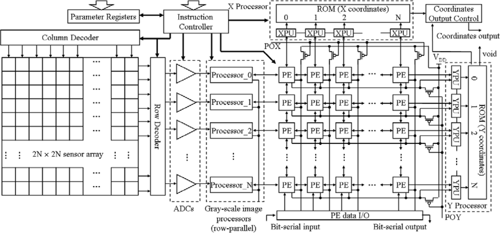
2.1. Architecture
2.2. Operations
2.2.1. Binary Mathematical Morphology
2.2.2. Gray-Scale Mathematical Morphology
2.2.3. Detecting a Void Image
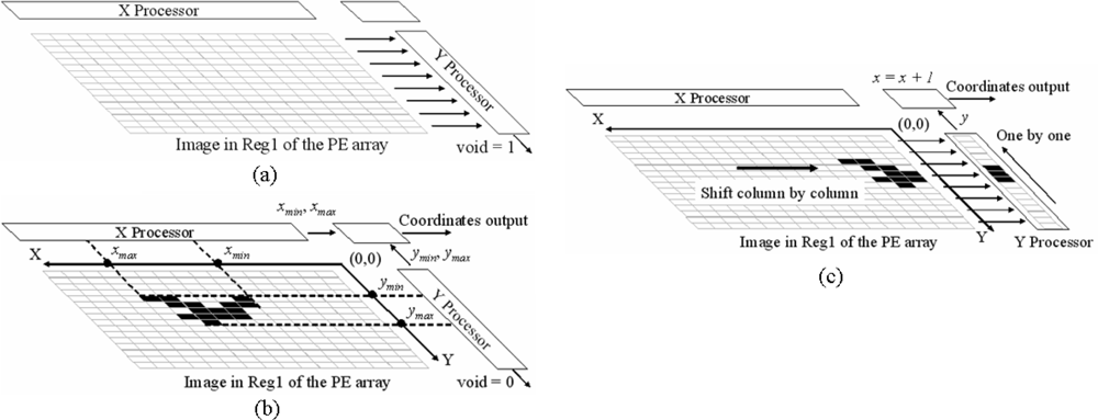
2.2.4. Extracting the Range and the Center of a Region
2.2.5. Extracting the Coordinates of Activated Pixels
3. VLSI Circuits Design
3.1. CMOS Image Sensor
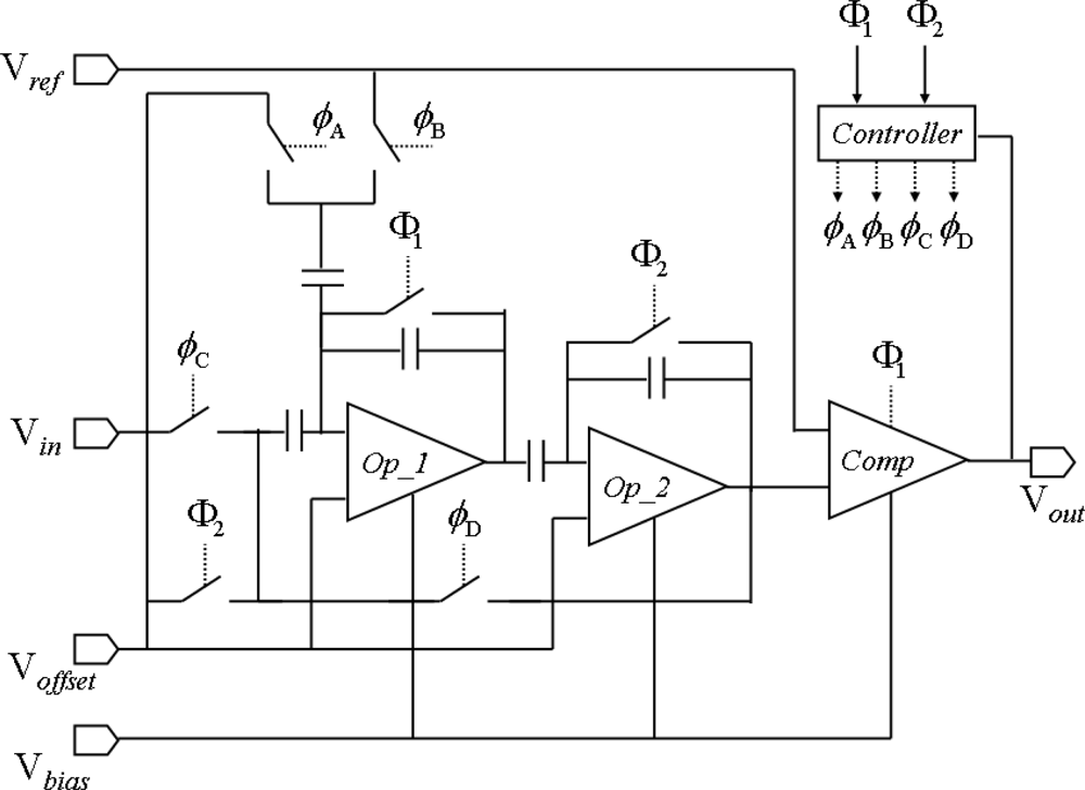
3.2. Row-Parallel 6-bit Algorithmic ADCs
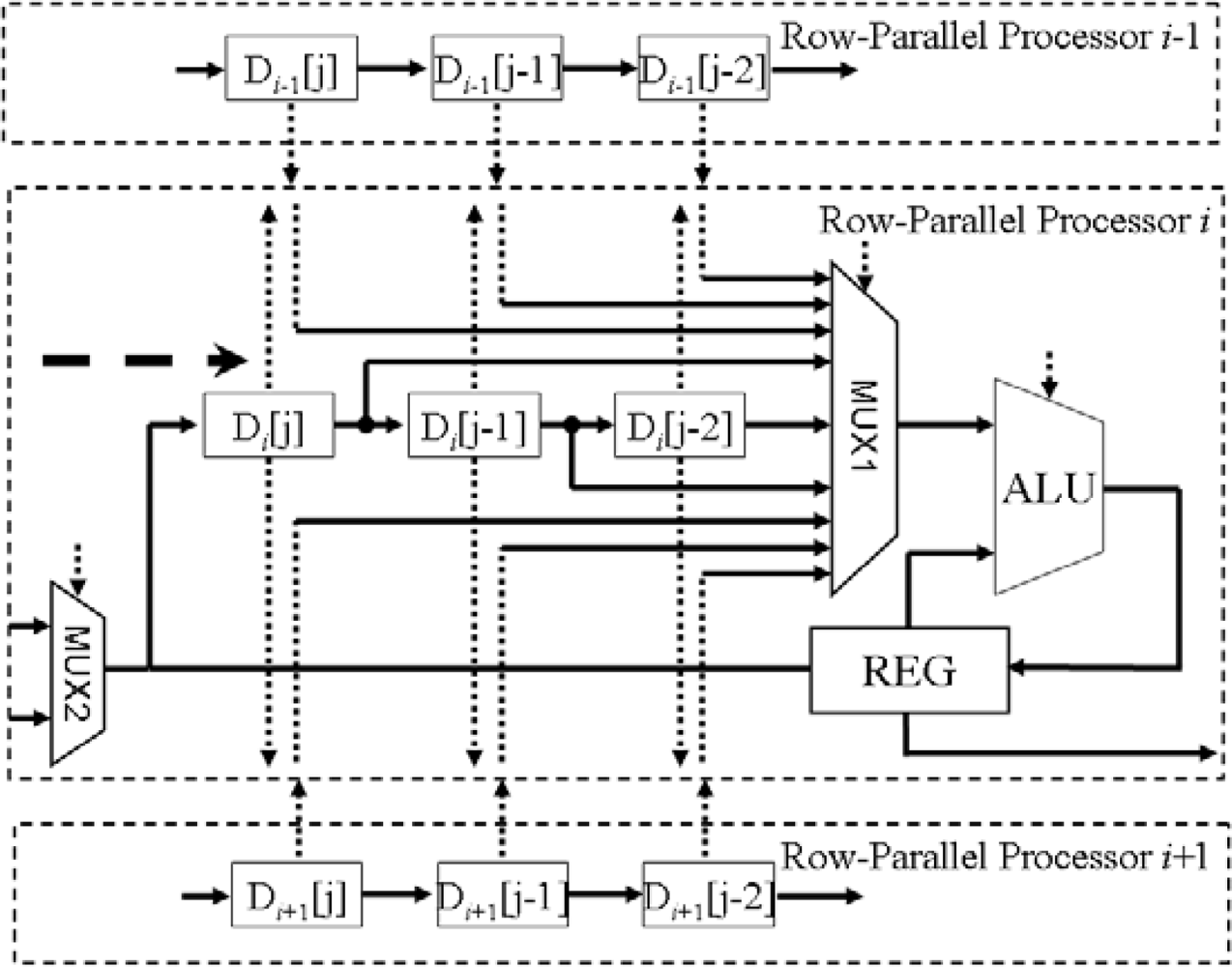
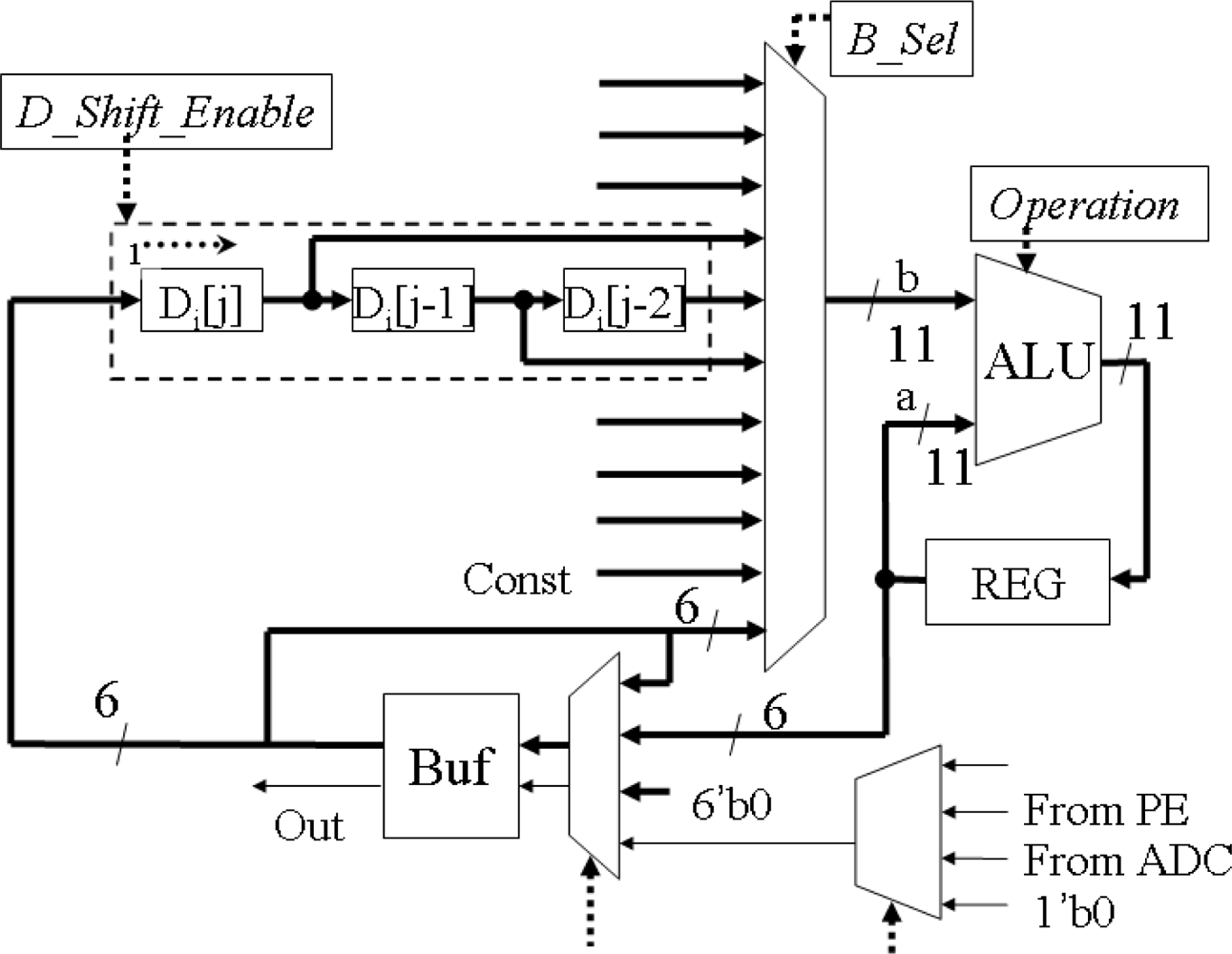
3.3. Row-Parallel Processors
3.4. Search Chain in X Processors and Y Processors
3.4.1. XPUs in the X Processor
3.4.2. YPUs in the Y Processor
4. Chip Implementation and Experiments
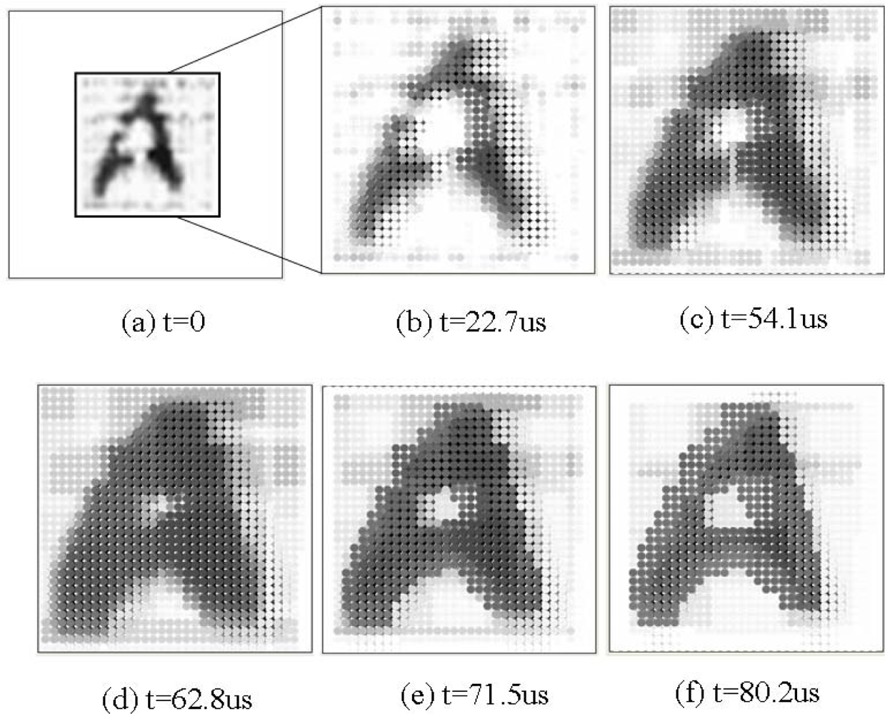
4.1. Experiment in Gray-Scale Mathematical Morphology
4.2. Experiment in Binary Mathematical Morphology
4.3. Target Tracking
5. Discussion of Performance
6. Conclusions
Acknowledgments
References and Notes
- Aizawa, K. Computational sensors—vision VLSI. IEICE Trans. Inf. Syst 1999, E82-D, 580–588. [Google Scholar]
- Seitz, P. Solid-state image sensing. In Handbook of Computer Vision and Applications; Academic Press: New York, USA, 2000; Volume 1, pp. 165–222. [Google Scholar]
- Gonzalez, R.C.; Woods, R.E. Digital Image Processing, 2nd ed; Pearson Education, Inc: Upper Saddle River, NJ, USA, 2002; p. 2. [Google Scholar]
- Yadid-Pecht, O.; Belenky, A. In-pixel Autoexposure CMOS APS. IEEE J. Solid-State Circ 2003, 38, 1425–1428. [Google Scholar]
- Acosta-Serafini, P.; Ichiro, M.; Sodini, C. A 1/3 VGA linear wide dynamic range CMOS image sensor implementing a predictive multiple sampling algorithm with overlapping integration intervals. IEEE J. Solid-State Circ 2004, 39, 1487–1496. [Google Scholar]
- Dudek, P.; Hicks, P.J. A general-purpose processor-per-pixel analog SIMD vision chip. IEEE Trans. Circ. Syst. I 2005, 52, 13–20. [Google Scholar]
- Kozlowski, L.; Rossi, G.; Blanquart, L.; Marchesini, R.; Huang, Y.; Chow, G.; Richardson, J.; Standley, D. Pixel noise suppression via soc management of target reset in a 1920 × 1080 CMOS image sensor. IEEE J. Solid-State Circ 2005, 40, 2766–2776. [Google Scholar]
- Massari, N.; Gottardi, M. A 100 dB dynamic-range CMOS vision sensor with programmable image processing and global feature extraction. IEEE J. Solid-State Circ 2007, 42, 647–657. [Google Scholar]
- Oike, Y.; Ikeda, M.; Asada, K. A row-parallel position detector for high-speed 3-D camera based on light-section method. IEICE Trans. Electron 2003, E86-C, 2320–2328. [Google Scholar]
- Oike, Y.; Ikeda, M.; Asada, K. A 375 × 365 1 k frames/s range-finding image sensor with 394.5 kHz access rate and 0.2 sub-pixel accuracy. ISSCC 2004, 1, 118–517. [Google Scholar]
- Komuro, T.; Ishii, I.; Ishikawa, M.; Yoshida, A. A digital vision chip specialized for high-speed target tracking. IEEE Trans. Electron. Dev 2003, 50, 191–199. [Google Scholar]
- Watanabe, Y.; Komuro, T.; Kagami, S.; Ishikawa, M. Vision chip architecture for simultaneous output of multi-target positions. Proceedings of SICE Annual Conference, Fukui, Japan, August 4–6, 2003; pp. 1572–1575.
- Luppe, M.; da Costa, L.F.; Roda, V.O. Parallel implementation of exact dilations and multi-scale skeletonization. J. Real-Time Imaging 2003, 9, 163–169. [Google Scholar]
- da Costa, L.F. Robust skeletonization through exact Euclidean distance transform and its applications to neuromorphometry. J. Real-Time Imaging 2003, 6, 415–431. [Google Scholar]
- Miao, W.; Lin, Q.; Wu, N. A novel vision chip for high-speed target tracking. Jpn. J. Appl. Phys 2007, 46, 2220–2225. [Google Scholar]
- Lin, Q.; Miao, W.; Wu, N. A high-speed target tracking CMOS image sensor. IEEE Asian Solid-State circuits Conference, Hangzhou, China, November, 2006; pp. 139–142.
- Zimmermann, H. Silicon Optoelectronic Integrated Circuits; Springer: Berlin, Germany, 2003; pp. 62–66. [Google Scholar]
- Yang, D.; Fowler, B.; Gamal, A.E. A nyquist-rate pixel-level ADC for CMOS image sensors. IEEE J. Solid-State Circ 1999, 34, 348–356. [Google Scholar]
- Loeliger, T.; Bachtold, P.; Binnig, G.K.; Cherubini, G.; Durig, U.; Eleftheriou, E.; Vettiger, P.; Uster, M.; Jackel, H. Cmos sensor array with cell-level analog-to-digital conversion for local probe data storage. Proceedings of the 28th European Solid-State Circuit Conference (ESSCIRC 2002), Florence, Italy, September 24–26, 2002; pp. 623–626.
- Harton, A.; Ahmed, M.; Beuhler, A.; Castro, F.; Dawson, L.; Herold, B.; Kujawa, G.; Lee, K.; Mareachen, R.; Scaminaci, T. High dynamic range CMOS image sensor with pixel level ADC and in situ image enhancement. Sensors and camera systems for scientific and industrial applications VI. Proc. SPIE 2005, 5677, 67–77. [Google Scholar]
- Chi, Y.; Mallik, U.; Choi, E.; Clapp, M.; Gauwenberghs, G.; Etienne-Cummings, R. CMOS Pixel-level ADC with change detection. Proc. Int. Symp. Circ. Syst 2006, 1647–1650. [Google Scholar]
- Furuta, M.; Nishikawa, Y.; Inoue, T.; Kawahito, S. A high-speed, high-sensitivity digital CMOS image sensor with a global shutter and 12-bit column-parallel cyclic A/D converters. IEEE J. Solid-State Circ 2007, 42, 766–774. [Google Scholar]
- Sartori, A.; Gottardi, M.; Maloberti, F.; Simoni, A.; Torelli, G. Analog-to-digital converters for optical sensor arrays. Proceedings of the Third International Conference on Electronics, Circuits, and Systems (ICECS ‘96), Rodos, Greece, October 13–16, 1996; pp. 939–942.
- Wu, C.; Shih, Y.; Lan, J.; Hsieh, C.; Huang, C.; Lu, J. Design, optimization, and performance analysis of new photodiode structures for CMOS Active-Pixel-Sensor (APS) imager applications. IEEE Sens. J 2004, 4, 135–144. [Google Scholar]
- Cembrano, G.; Rodriguez-Vazquez, A.; Galan, R.; Jimenez-Garrido, F.; Espejo, S.; Dominguez-Castro, R. A 1000 fps at 128 × 128 vision processor with 8bit digitized I/O. IEEE J. Solid-State Circ 2004, 39, 1044–1055. [Google Scholar]
- Brea, V.M.; Vilariño, D.L.; Paasio, A.; Cabello, D. “Design of the processing core of a mixed-signal CMOS DTCNN chip for pixel-level snakes”. IEEE Trans. Circ. Syst. I 2004, 51, 997–1013. [Google Scholar]
- Sugiyama, Y.; Takumi, M.; Tyoda, H.; Mukozaka, N.; Ihori, A.; Kurashina, T.; Nakamura, Y.; Tonbe, T.; Mizuno, S. A high-speed CMOS image with profile data acquiring function. IEEE J. Solid-State Circ 2005, 40, 2816–2823. [Google Scholar]


| Operations | Clock cycles |
|---|---|
| Load from ADC | ≈8 × N |
| Shift 1 pixel | 1 |
| Copy | 1 |
| AND/OR/NOT | 1 |
| Binary Erosion / Dilation | ≈M(1) |
| Gray-scale Erosion / Dilation | ≈M × N(2) |
| Detecting a void image | 2 |
| Extracting the Range and the center | 8 |
| Extracting coordinates of activated pixels | ≈2K(3) |
| Bit-serial binary image input/output | ≈N × N |
| Parameter | Value |
|---|---|
| Technology | 0.18 μm 1P6M CMOS Std. |
| Chip Size (pad incl.) | 3.5 mm × 1.5 mm |
| Array Size | 64 × 64 pixels for Sensor Array |
| 32 × 32 pixels for PE Array | |
| Pixel Size | 9.5 μm × 9.5 μm for Sensor |
| 23 μm × 29 μm for PE | |
| Number of trans/pixel | 3 trans in Sensor pixel |
| 85 trans in PE pixel | |
| Fill Factor | 58% |
| Clock frequency | 40 MHz |
| Power supply and consumption | 1.8 V & 3.3V |
| 82.5mW (@, 1,000 fps) |
| Reference | Our chip | [13] | [25] | [26] | [27] |
|---|---|---|---|---|---|
| Photosensors | Yes | No | Yes | Yes | Yes |
| Technology | 0.18 μm 1P6M | FPGA | 0.35 μm 1P5M | 0.25 μm | 0.6 μm 2P3M |
| PE area (μm2) | 23 × 29 | 68 LE* | 75.5 × 73.3 | 83 × 45 | 20 × 20 |
| Stored bits per PE | 8 | N/A | 32 | 4 | N/A |
| PE Array | 32 × 32 | 12 × 12 | 128 × 128 | 9 × 9 | 512 × 512 |
| Image processing | 6-Bit Gray | 9-Bit Gray | 8-Bit Gray | 4-Bit Gray | Analog |
| Control Style | SIMD | Regular | SIMD/CNN | Complicated | Regular |
| Global features | Specific periphery | N/A | Non-specific Periphery | No exportation | Specific periphery |
| Programmability | High | Specific | High | Moderate | Low |
© 2009 by the authors; licensee MDPI, Basel, Switzerland This article is an open access article distributed under the terms and conditions of the Creative Commons Attribution license (http://creativecommons.org/licenses/by/3.0/).
Share and Cite
Lin, Q.; Miao, W.; Zhang, W.; Fu, Q.; Wu, N. A 1,000 Frames/s Programmable Vision Chip with Variable Resolution and Row-Pixel-Mixed Parallel Image Processors. Sensors 2009, 9, 5933-5951. https://doi.org/10.3390/s90805933
Lin Q, Miao W, Zhang W, Fu Q, Wu N. A 1,000 Frames/s Programmable Vision Chip with Variable Resolution and Row-Pixel-Mixed Parallel Image Processors. Sensors. 2009; 9(8):5933-5951. https://doi.org/10.3390/s90805933
Chicago/Turabian StyleLin, Qingyu, Wei Miao, Wancheng Zhang, Qiuyu Fu, and Nanjian Wu. 2009. "A 1,000 Frames/s Programmable Vision Chip with Variable Resolution and Row-Pixel-Mixed Parallel Image Processors" Sensors 9, no. 8: 5933-5951. https://doi.org/10.3390/s90805933