On the Capability of Artificial Neural Networks to Compensate Nonlinearities in Wavelength Sensing

Abstract
:
1. Introduction
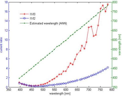
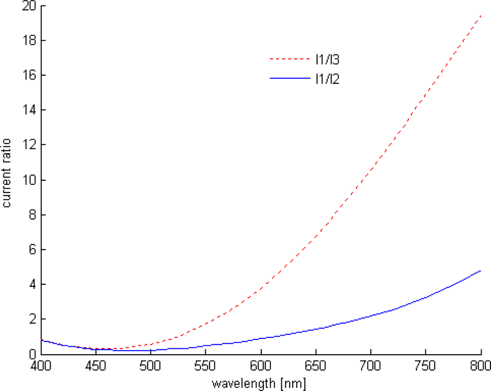
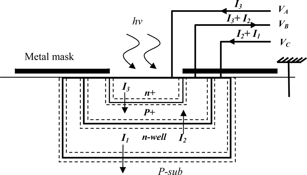
2. Modeling and Problem Formulation
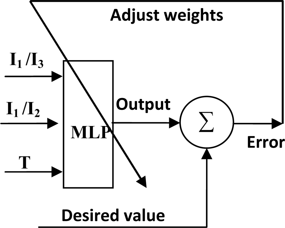
3. ANN Based-on Signal Readout
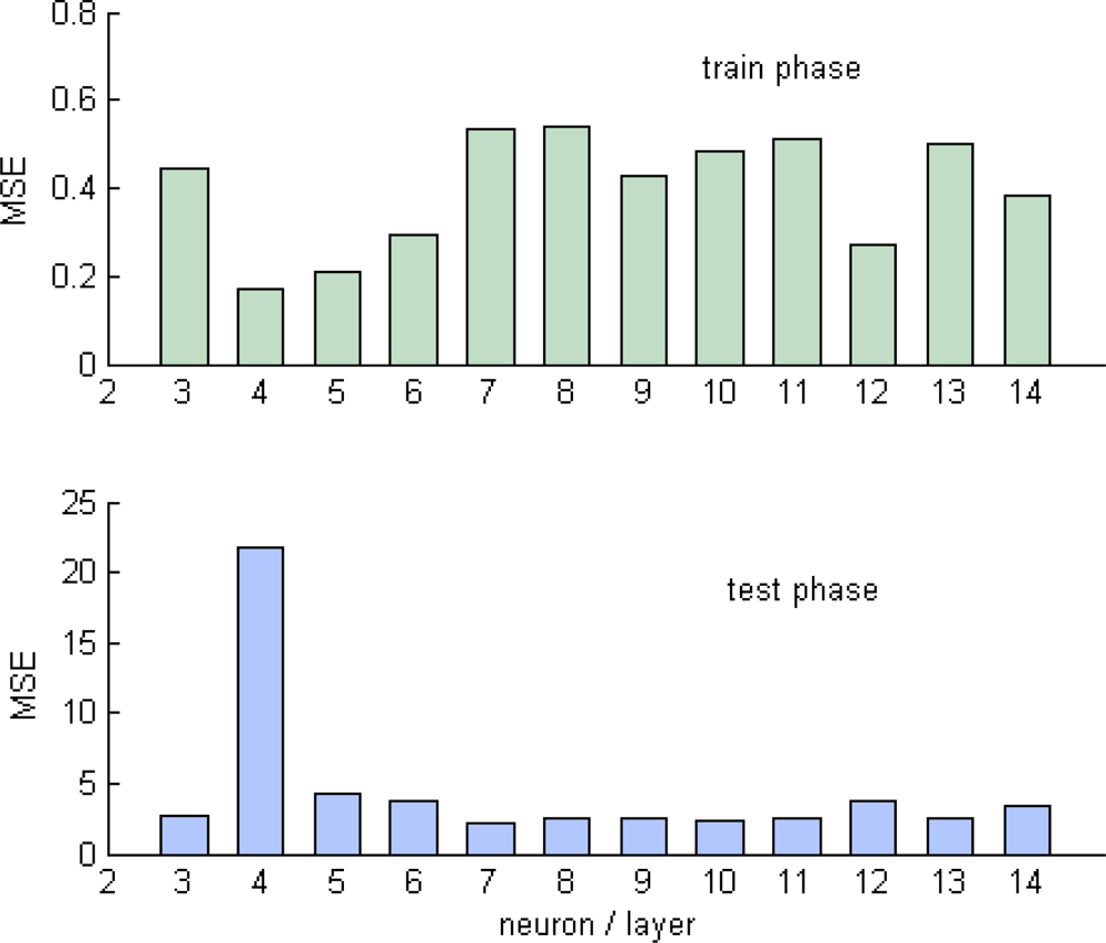
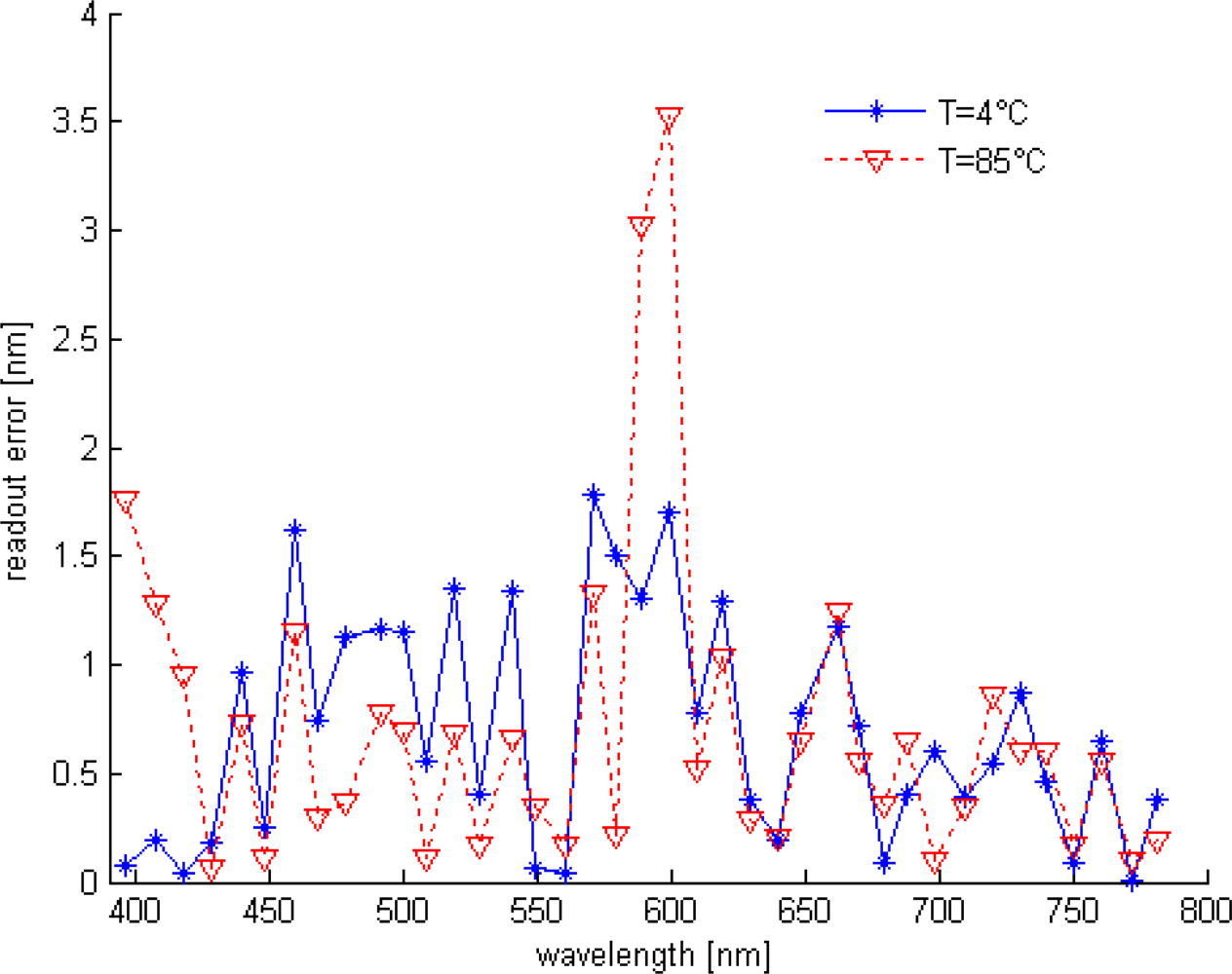
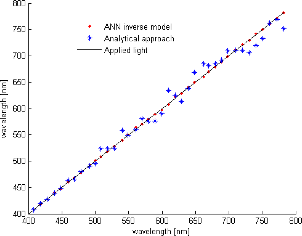
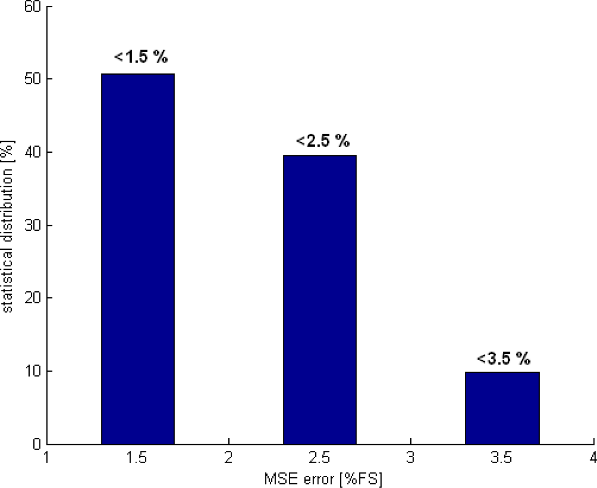
4. Implementation and Simulation Results
5. Conclusions
Acknowledgments
References and Notes
- Chouikha, M.B.; Lu, G.N.; Sedjil, M.; Sou, G. Colour detection using buried triple pn junction structure implemented in BiCMOS process. Electron. Lett 1998, 34, 120–122. [Google Scholar]
- Sangwine, S.J.; Horne, R.E.N. The Color Image Processing Handbook; Springer: New York, NY, USA, 1998. [Google Scholar]
- Dillon, P.L.; Brault, A.T.; Horak, J.R.; Garcia, E.; Martin, T.W.; Light, W.A. Fabrication and performance of colour filter arrays for solid-state imagers. IEEE Trans. Electron. Dev 1978, 25, 97–101. [Google Scholar]
- Pau, L.F.; Johansen, F.S. Neural network signal understanding for instrumentation. IEEE Trans. Instrum. Meas 1990, 39, 558–564. [Google Scholar]
- Daponte, P.; Grimaldi, D. Artificial neural networks in measurements. Measurement 1998, 23, 93–115. [Google Scholar]
- Hu, Y.H.; Hwang, J.N. Handbook of Neural Network Signal Processing; CRC Press: Washington, DC, USA, 2002. [Google Scholar]
- Dias Pereira, J.M.; Girao, P.M.B.; Postolache, O. Fitting transducer characteristics to measured data. IEEE Instrum. Meas. Mag 2001, 4, 26–39. [Google Scholar]
- Patra, J.C.; Kot, A.C.; Panda, G. An intelligent pressure sensor using neural networks. IEEE Trans. Instrum. Meas 2000, 49, 829–834. [Google Scholar]
- Patra, J.C.; van den Bos, A.; Kot, A.C. An ANN-based smart capacitive pressure sensor in dynamic environment. Sens. Actuat. A 2000, 86, 26–38. [Google Scholar]
- Dias Pereira, J.M.; Postolache, O.; Silva Girao, P.M.B. A temperature-compensated system for magnetic field measurements based on artificial neural networks. IEEE Trans. Instrum. Meas 1998, 47, 494–498. [Google Scholar]
- Carullo, A.; Ferraris, F.; Graziani, S.; Grimaldi, U.; Parvis, M. Ultrasonic distance sensor improvement using a two-level neural-network. IEEE Trans. Instrum. Meas 1996, 45, 677–682. [Google Scholar]
- Tian, G.Y. Design and implementation of distributed measurement systems using fieldbus-based intelligent sensors. IEEE Trans. Instrum. Meas 2000, 50, 1197–1202. [Google Scholar]
- Arpaia, P.; Daponte, P.; Grimaldi, D.; Michaeli, L. ANNbased error reduction for experimentally modeled sensors. IEEE Trans. Instrum. Meas 2002, 51, 23–30. [Google Scholar]
- Hafiane, M.L.; Dibi, Z.; Saidi, L.; Hafiane, A. Modeling of a capacitive pressure sensor using artificial neural networks. Proceedings of the IEEE ICTTA’06, Damascus, Syria, 24–28 April, 2006; p. 73.
- Patra, J.C.; Ang, E.L.; Chaudhari, N.S.; Das, A. Neural-network-based smart sensor framework operating in a harsh environment. EURASIP J. Appl. Signal Proc 2005, 4, 558–574. [Google Scholar]
- Rivera, J.; Carrillo, M.; Chacón, M.; Herrera, G.; Bojorquez, G. Self-calibration and optimal response in intelligent sensors design based on artificial neural networks. Sensors 2007, 7, 1509–1529. [Google Scholar]
- Dias Pereira, J.M.; Postolache, O.; Silva Girao, P.M.B. A temperature-compensated system for magnetic field measurements based on artificial neural networks. IEEE Trans. Instrum. Meas 1998, 47, 494–498. [Google Scholar]
- Carullo, A.; Ferraris, F.; Graziani, S.; Grimaldi, U.; Parvis, M. Ultrasonic distance sensor improvement using a two-level neural-network. IEEE Trans. Instrum. Meas 1996, 45, 677–682. [Google Scholar]
- Tian, G.Y. Design and implementation of distributed measurement systems using fieldbus-based intelligent sensors. IEEE Trans. Instrum. Meas 2001, 50, 1197–1202. [Google Scholar]
- Arpaia, P.; Daponte, P.; Grimaldi, D.; Michaeli, L. ANN-based error reduction for experimentally modeled sensors. IEEE Trans. Instrum. Meas 2002, 51, 23–30. [Google Scholar]
- Alexandre, A.; Sou, G.; Chouikha, M.B.; Sedjil, M.; Lu, G.N.; Aiquie, G. Modeling and design of multi buried junctions detector for color systems development. Proceedings of Symposium on Design, Test, Integration, and Packaging of MEMS/MOEMS, Paris, France, 9–11 May 2000; 4019, pp. 288–298.
- Lu, G.N. A dual-wavelength method using the BDJ detector and its application to iron concentration measurement. Meas. Sci. Technol 1999, 10, 312–315. [Google Scholar]
- Lu, G.N.; Guillaud, G.; Sou, G.; Devigny, F.; Pitaval, M.; Morin, P. Investigation of CMOS BDJ detector for fluorescence detection in microarray analysis. Proceedings of 1st Annual International Conference On Microtechnologies in Medicine and Biology, Lyon, France, 12–14 December, 2000; pp. 381–386.
- Hornik, K.; Stinchcombe, M.; White, H. Multilayer feedforward networks are universal approximators. Neur. Netw 1989, 2, 359–366. [Google Scholar]
- Funahashi, K.I. On the approximate realization of continuous mappings by neural networks. Neur. Netw 1989, 2, 193–192. [Google Scholar]


| Parameters | Optimized values | |
|---|---|---|
| Architecture | Normal feed-forward MLP | |
| Hidden layer | 1 | |
| Training algorithm | Back-propagation | |
| Number of neurons | Input layer | 3 |
| Hidden layer | 7 | |
| Output layer | 1 | |
| Transfer function | Hidden layer | Sigmoid |
| Output layer | Linear | |
| Output range | Wavelength (nm) | |
| Max | 780 | |
| Min | 400 | |
| Data base size | Training set | 234 |
| Test set | 36 | |
© 2009 by the authors; licensee MDPI, Basel, Switzerland This article is an open access article distributed under the terms and conditions of the Creative Commons Attribution license (http://creativecommons.org/licenses/by/3.0/).
Share and Cite
Hafiane, M.L.; Dibi, Z.; Manck, O. On the Capability of Artificial Neural Networks to Compensate Nonlinearities in Wavelength Sensing. Sensors 2009, 9, 2884-2894. https://doi.org/10.3390/s90402884
Hafiane ML, Dibi Z, Manck O. On the Capability of Artificial Neural Networks to Compensate Nonlinearities in Wavelength Sensing. Sensors. 2009; 9(4):2884-2894. https://doi.org/10.3390/s90402884
Chicago/Turabian StyleHafiane, Mohamed Lamine, Zohir Dibi, and Otto Manck. 2009. "On the Capability of Artificial Neural Networks to Compensate Nonlinearities in Wavelength Sensing" Sensors 9, no. 4: 2884-2894. https://doi.org/10.3390/s90402884