Measuring Gait Using a Ground Laser Range Sensor


Abstract
:
1. Introduction
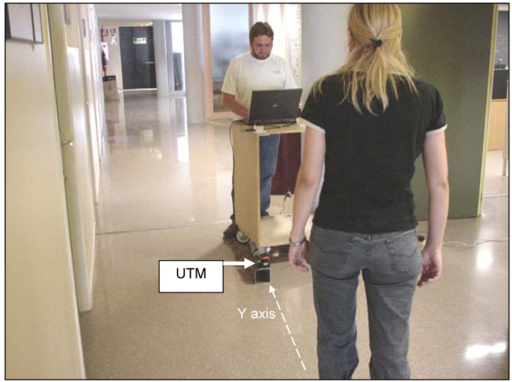
2. Measurement System
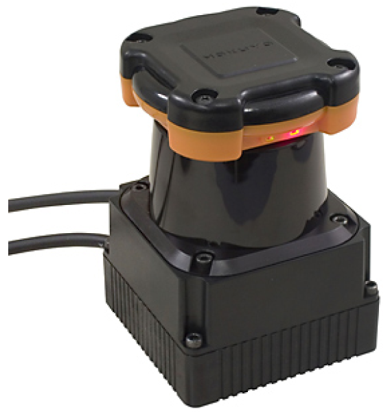
2.1. Laser Range Sensor
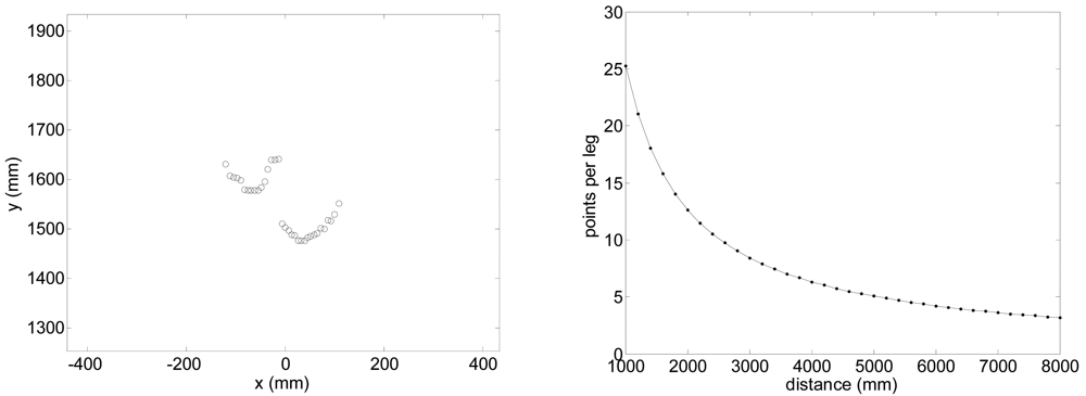
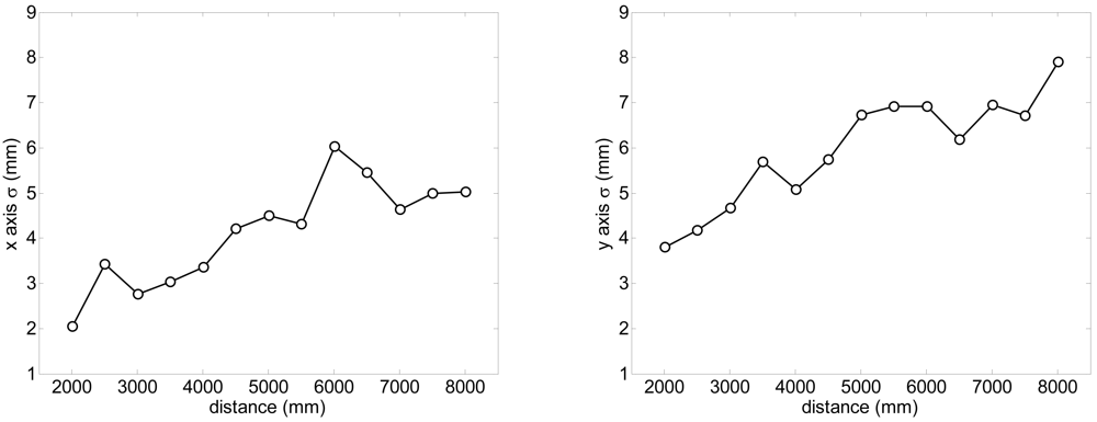
2.2. Range measurement
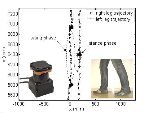
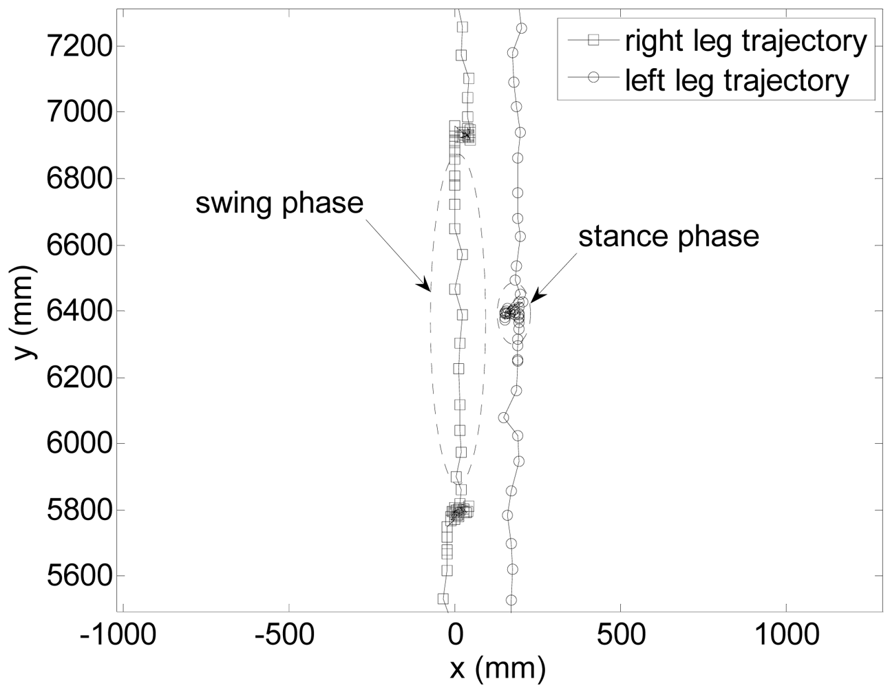
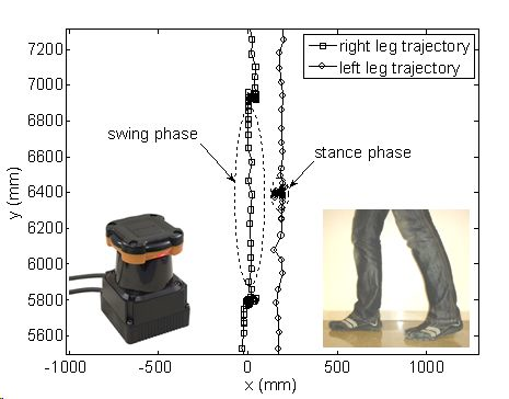
2.3. Estimating the Position of the Legs
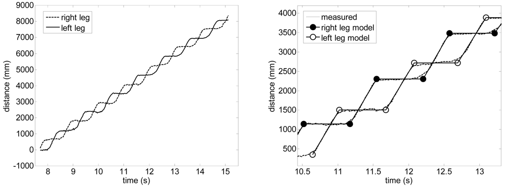
2.4. Step-Line Model of the Gait
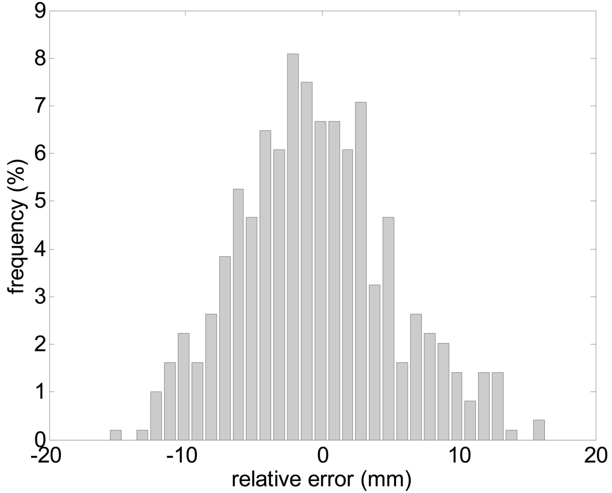
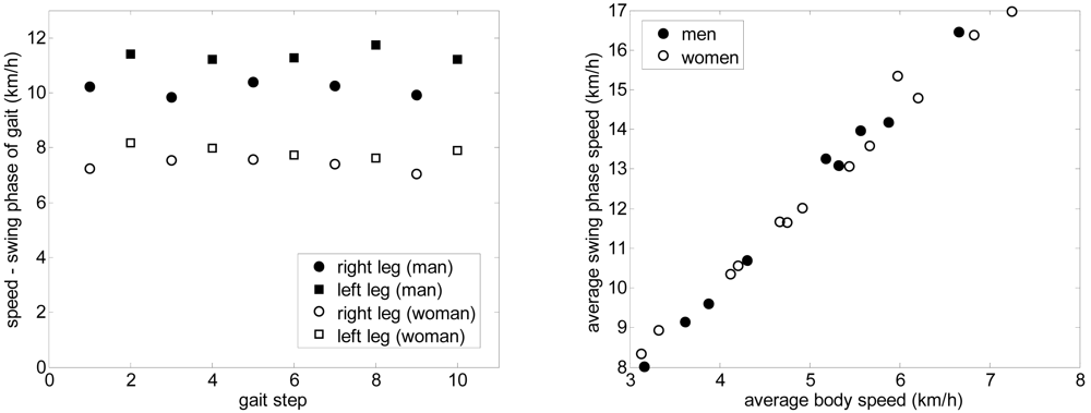
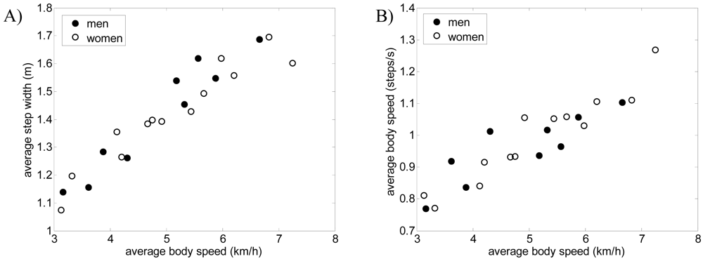
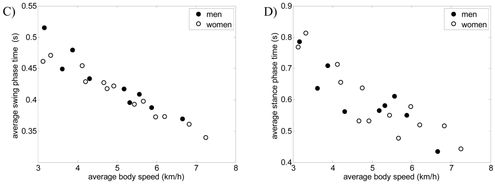
3. Results
4. Conclusions and Future Work
References and Notes
- Brooks, P. Body Work; Harvard University Press: Cambridge, MA, USA, 1993. [Google Scholar]
- Guyton, A. Function of the human body, 4th ed.; Saunders: Philadelphia, PA, USA, 1974. [Google Scholar]
- Martorell, R. Body size, adaptation and function. Hum. Organ. 1989, 48, 15–20. [Google Scholar]
- Lim, I.; Wegen, E.; Goede, C.; Deutekom, M.; Nieuwboer, A.; Willems, A.; Jones, D.; Rochester, L.; Kwakkel, G. Effects of external rhythmical cueing on gait in patients with Parkinson's disease: a systematic review. Clin. Rehabil. 2005, 19, 695–713. [Google Scholar]
- Morris, M.E. Movement disorders in people with Parkinson disease: a model for physical therapy. Phys. Ther. 2000, 80, 578–597. [Google Scholar]
- Cutting, J.; Kozlowski, L. Recognising friends by their walk: gait perception without familiarity cues. Bull. Psychonomic Soc. 1977, 9, 353–356. [Google Scholar]
- Little, J.; Boyd, J. Recognizing people by their gait: the shape of motion. Videre 1998, 1, 2–32. [Google Scholar]
- Kozlowski, L.; Cutting, J. Recognizing the sex of a walker from a dynamic point-light display. Percept. Psychophys. 1977, 21, 575–580. [Google Scholar]
- Hausdorff, J.M.; Rios, D.A.; Edelberg, H.K. Gait variability and fall risk in community-living older adults: a 1-year prospective study. Arch. Phys. Med. Rehabil. 2001, 82, 1050–1056. [Google Scholar]
- Wang, L. Abnormal walking gait analysis using silhouette-masked flow histograms. Proceedings of the 18th International Conference on Pattern Recognition, Hong Kong, August 20-24, 2006; pp. 473–476.
- Mayagoitia, R.E.; Nene, A.V.; Veltink, P.H. Accelerometer and rate gyroscope measurement of kinematics: an inexpensive alternative to optical motion analysis systems. J. Biomech. 2002, 35, 537–542. [Google Scholar]
- Bamberg, S.; Benbasat, A.Y.; Scarborough, D.M.; Krebs, D.E.; Paradiso, J.A. Gait analysis using a shoe-integrated wireless sensor system. IEEE Trans. Inform. Technol. Biomed. 2008, 12, 413–423. [Google Scholar]
- Qian, G.; Zhang, J.; Kidane, A. People identification using gait via floor pressure sensing and analysis. Lect. Note. Comput. Sci. 2008, 5279, 83–98. [Google Scholar]
- Farjas, M.; Sillero-Quintana, M.; Merino, P.A. Applying topographic techniques to modeling the human shape in motion. Second Workshop on Digital Media and its Application in Museum & Heritages, Chongqing, China, December 10-12, 2007; pp. 169–172.
- Gate, G.; Nashashibi, F. Using targets appearance to improve pedestrian classification with a laser scanner. IEEE Intelligent Vehicles Symposium, Eindhoven, The Netherlands, June 4-6, 2008; pp. 571–576.
- Navarro-Serment, L.E.; Mertz, C.; Hebert, H. Pedestrian detection and tracking using three-dimensional ladar data. Proceedings of the 7th International Conference on Field and Service Robotics, Cambridge, MA, USA, July 14-16, 2009.
- Gidel, S.; Blanc, C.; Chateau, T.; Checchin, P.; Trassoudaine, L. A method based on multilayer laserscanner to detect and track pedestrians in urban environment. IEEE Intelligent Vehicles Symposium, Xi'an, Shaanxi, China, June 3-5, 2009; pp. 157–162.
- Morales, Y.; Takeuchi, E.; Carballo, A.; Tokunaga, W.; Kuniyoshi, H.; Aburadani, A.; Hirosawa, A.; Nagasaka, Y.; Suzuki, Y.; Tsubouchi, T. 1 km autonomous robot navigation on outdoor pedestrian paths “running the tsukuba challenge”. Proceedings of International Conference on Intelligent Robots and Systems, Nice, France, September 22-26, 2008; pp. 219–225.
- Vázquez-Martín, R.; Núñez, P.; Bandera, A.; Sandoval, F. Curvature-based environment description for robot navigation using laser range sensors. Sensors 2009, 9, 5894–5918. [Google Scholar]
- Palacín, J.; Palleja, T.; Tresanchez, M.; Sanz, R.; Llorens, J.; Ribes-Dasi, M.; Masip, J.; Arnó, J.; Escola, A.; Rosell, J.R. Real-time tree-foliage surface estimation using a ground laser scanner. IEEE Trans. Instrum. Meas. 2007, 56, 1377–1383. [Google Scholar]
- Voss, M.; Sugumaran, R. Seasonal effect on tree species classification in an urban environment using hyperspectral data, lidar, and an object-oriented approach. Sensors 2008, 8, 320–336. [Google Scholar]
- Swanson, A.; Huang, S.; Crabtree, R. Using a LIDAR vegetation model to predict UHF SAR attenuation in coniferous forests. Sensors 2009, 9, 1559–1573. [Google Scholar]
- Hokuyo Automatic Co., Ltd. Scanning Laser Range Finder UTM-30LX/LN Specification, Drawing No. C-42-3615; 2008. [Google Scholar]
- Ahn, S.J.; Rauh, W.; Warnecke, H. Least-squares orthogonal distances fitting of circle, sphere, ellipse, hyperbola, and parabola. Pattern Recognit. 2001, 34, 2283–2303. [Google Scholar]
- Whittle, M.W. Gait analysis: An introduction; Elsevier Health Sciences: Oxford, UK, 2002. [Google Scholar]


| Parameter | Typical value |
|---|---|
| Power source | 12V ±10% |
| Current consumption | 0.7A (rush current 1.0A) |
| Detection range | 0.1 to approx. 60 m (<30 m guaranteed) |
| Laser wavelength | 870 nm, Class 1 |
| Eye safe | |
| Scan angle | 270° |
| Scan time | 0.025 s/scan (40.0 Hz) |
| Angular Resolution | 0.25° |
| Interface | USB 2.0 |
| Serial COM | |
| Weight | 0.233 kg |
| Measurement error | 0.1 to 10 m (±30 mm) |
| 10 to 30 m (±50 mm) |
© 2009 by the authors; licensee Molecular Diversity Preservation International, Basel, Switzerland. This article is an open access article distributed under the terms and conditions of the Creative Commons Attribution license (http://creativecommons.org/licenses/by/3.0/).
Share and Cite
Pallejà, T.; Teixidó, M.; Tresanchez, M.; Palacín, J. Measuring Gait Using a Ground Laser Range Sensor. Sensors 2009, 9, 9133-9146. https://doi.org/10.3390/s91109133
Pallejà T, Teixidó M, Tresanchez M, Palacín J. Measuring Gait Using a Ground Laser Range Sensor. Sensors. 2009; 9(11):9133-9146. https://doi.org/10.3390/s91109133
Chicago/Turabian StylePallejà, Tomàs, Mercè Teixidó, Marcel Tresanchez, and Jordi Palacín. 2009. "Measuring Gait Using a Ground Laser Range Sensor" Sensors 9, no. 11: 9133-9146. https://doi.org/10.3390/s91109133