New Method for Estimation of Aeolian Sand Transport Rate Using Ceramic Sand Flux Sensor (UD-101)

Abstract
:1. Introduction
- The sensor is calibrated by performing both wind tunnel and field experiments.
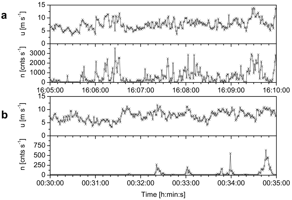
- The sensor records an impact value of 0 or 1 at 10 kHz; it samples once per second, and theoretically, it can detect a maximum of 10,000 impact counts in the sampling interval, i.e., the sensor has high temporal resolution.
- The sensor is relatively inexpensive.
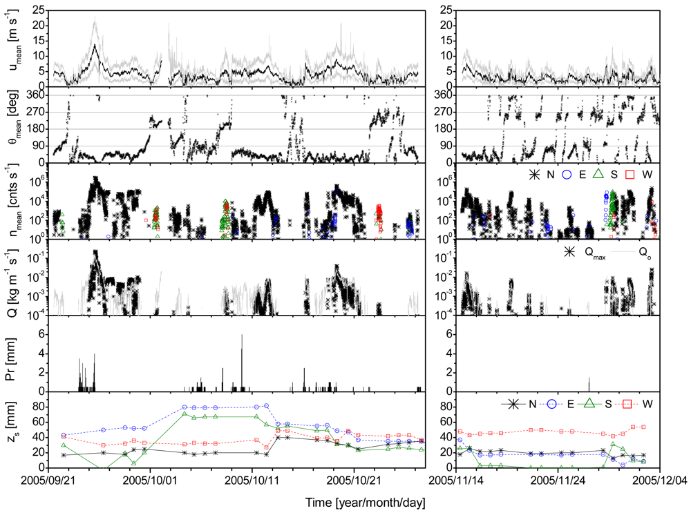
- During periods without rainfall and in the presence of longshore winds (conditions similar to those employed in wind tunnel experiments), the aeolian sand flux at a certain height above a flat ground surface increased significantly with the wind velocity and approximately equaled the flux estimated in wind tunnel experiments using Kawamura's [3] equation.
- The flux decreased significantly with an increase in precipitation, i.e., with an increase in the moisture content of the sand surface; however, even during periods with rainfall, flux was detected during strong wind conditions.
- The flux increased with a decrease in the angle between the sensor direction and wind direction.
2. New Estimation Method for Determining Total Aeolian Sand Flux
2.1. Characteristics of UD-101 Data
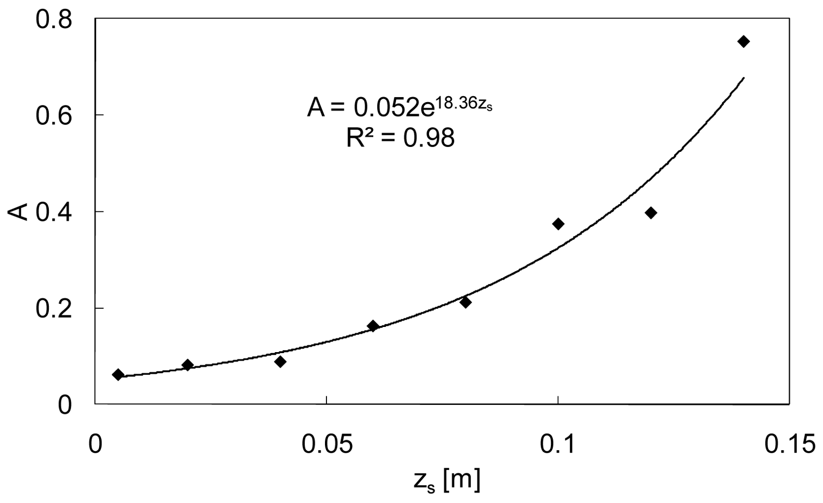
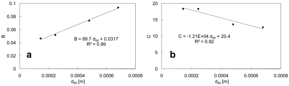
2.2. Relationship between Impact Counts and Aeolian Sand Flux at a Measurement Height
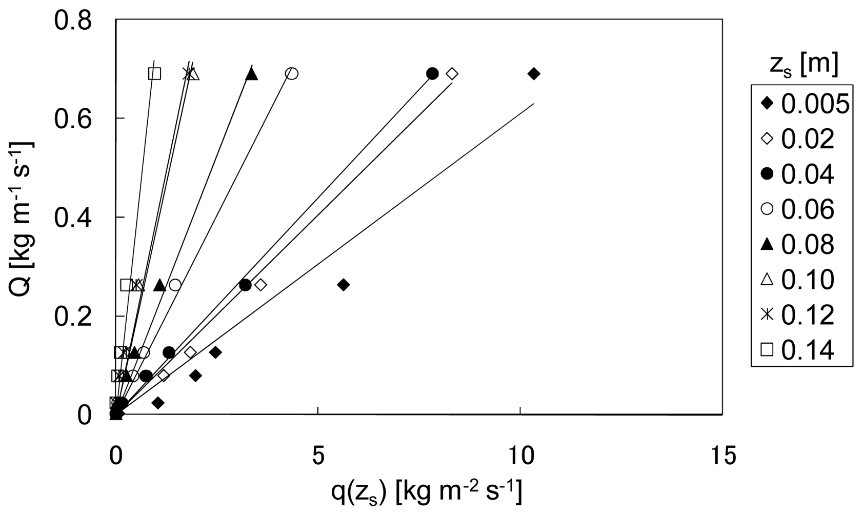
2.3. Relationship between Aeolian Sand Flux at a Measurement Height and Total Sand Flux
3. UD-101 Data Obtained at Hasaki Beach
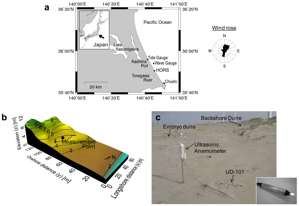
3.1. Summary of Field Measurements
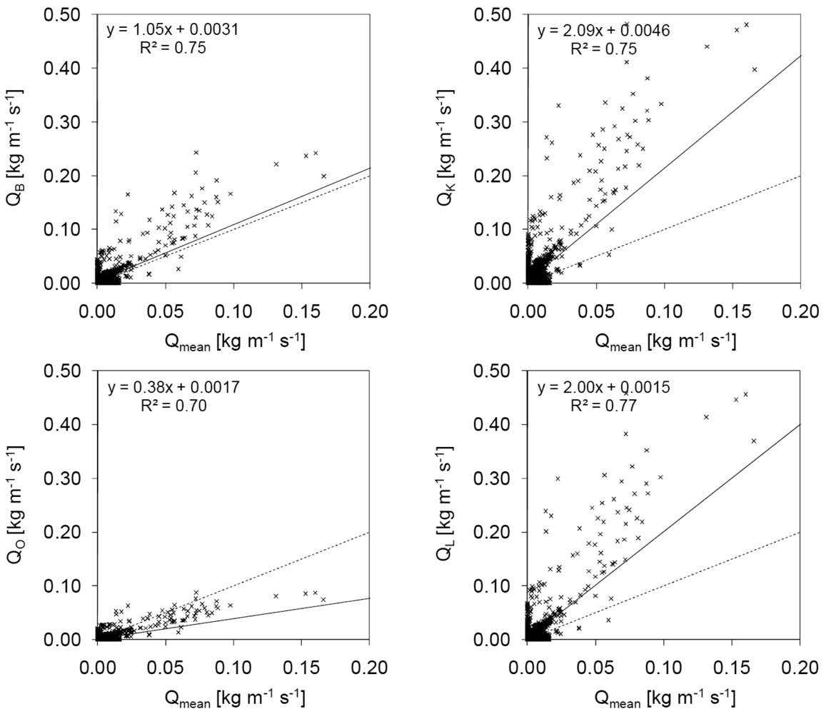
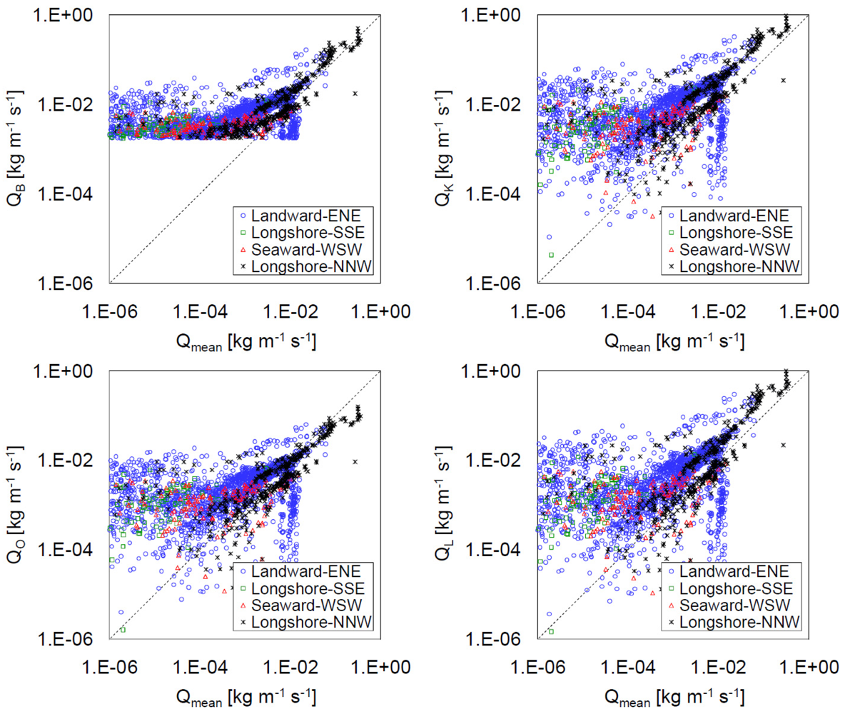
3.2. Evaluation of the Accuracy of the New Method by Comparing Q with QB, QK, QO, and QL
4. Conclusions
Acknowledgments
References and Notes
- Bagnold, R.A. The Physics of Blown Sand and Desert Dunes; Methuen: London, UK, 1941; p. 265. [Google Scholar]
- Chepil, W. Dynamics of wind erosion. II: initiation of soil movement. Soil Sci. 1945, 6, 397–411. [Google Scholar]
- Kawamura, R. Study of sand movement by wind. Univ. Tokyo, Rep. Inst. Sci. Technol. 1951, 5, 95–112. (in Japanese). [Google Scholar]
- Zingg, A.W. Wind tunnel studies of the movement of sedimentary material. Proceedings of 5th Hydraulic Conference, Iowa City, IA, USA; McNown, J.S., Boyer, M.C., Eds.; Iowa Institute of Hydraulic Research, State University of Iowa, 1953; pp. 111–135. [Google Scholar]
- Owen, P.R. Saltation of uniform grains in air. J. Fluid Mech. 1964, 20, 225–242. [Google Scholar]
- Letau, K.; Lettau, H.H. Experimental and micrometeorological field studies of dune migration. In Exploring the World's Driest Climates; Lettau, H.H., Lettau, K., Eds.; Institute of Environmental Science Report 101, Center for Climatic Research, University of Wisconsin: Madison, WI, USA, 1978; pp. 110–147. [Google Scholar]
- White, B.R. Soil transport by winds on Mars. J. Geophys. Res. 1979, 84, 4643–4651. [Google Scholar]
- Iversen, J.D.; White, B.R. Saltation threshold on Earth, Mars and Venus. Sedimentology 1982, 29, 111–119. [Google Scholar]
- Unger, J.E.; Haff, P.K. Steady state saltation in air. Sedimentology 1987, 34, 289–299. [Google Scholar]
- Werner, B.T. A steady-state model of wind-blown sand transport. J. Geol. 1990, 98, 1–17. [Google Scholar]
- Anderson, R.S.; Haff, P.K. Wind modification and bed response during saltation of sand in air. Acta Mech. 1991, 1, 21–51. [Google Scholar]
- Shao, Y.; Raupach, M.R. The overshoot and equilibrium of saltation. J. Geophys. Res. 1992, 97, 20559–20564. [Google Scholar]
- Iversen, J.D.; Rasmussen, K.R. The effect of wind speed and bed slope on sand transport. Sedimentology 1999, 46, 723–731. [Google Scholar]
- Shao, Y.; Lu, H. A simple expression for wind erosion threshold friction velocity. J. Geophys. Res. 2000, 105, 22437–22432. [Google Scholar]
- Roney, J.A.; White, B.R. Definition and measurement of dust aeolian thresholds. J. Geophys. Res. 2004, 109, F01013. [Google Scholar]
- Sorensen, M. On the rate of aeolian sand transport. Geomorphology 2004, 59, 53–62. [Google Scholar]
- Stockton, P.H.; Gillette, D.A. Field measurement of the sheltering effect of vegetation on erodible land surfaces. Land Degrad. Rehabil. 1990, 2, 77–85. [Google Scholar]
- Stout, J.E.; Zobeck, T.M. Intermittent saltation. Sedimentology 1997, 44, 959–970. [Google Scholar]
- Baas, A.C.W. Evaluation of saltation flux impact responders (Safires) for measuring instantaneous aeolian sand transport intensity. Geomorphology 2004, 59, 99–118. [Google Scholar]
- Gillies, J.A.; Berkofsky, L. Eolian suspension above the saltation layer, the concentration profile. J. Sediment. Res. 2004, 74, 176–183. [Google Scholar]
- Mikami, M.; Shi, G.Y.; Uno, I.; Yabuki, S.; Iwasaka, Y.; Yasui, M.; Aoki, T.; Tanaka, T.Y.; Kurosaki, Y.; Masuda, K.; Uchiyama, A.; Matsuki, A.; Sakai, T.; Takemi, T.; Nakawo, M.; Seino, N.; Ishizuka, M.; Satake, S.; Fujita, K.; Hara, Y.; Kai, K.; Kanayama, S.; Hayashi, M.; Du, M.; Kanai, Y.; Yamada, Y.; Zhang, X.Y.; Shen, Z.; Zhou, H.; Abe, O.; Nagai, T.; Tsutsumi, Y.; Chiba, M.; Suzuki, J. Aeolian dust experiment on climate impact: an overview of Japan-China joint project ADEC. Global Planet. Change. 2006, 52, 142–172. [Google Scholar]
- Udo, K.; Kuriyama, Y.; Jackson, D.W.T. Observations of wind-blown sand under various meteorological conditions. J. Geophys. Res. 2008, 113, F04008. [Google Scholar]
- Butterfield, G.R. Grain transport rates in steady and unsteady turbulent airflows. Acta Mech. 1991, 1, 97–122. [Google Scholar]
- Butterfield, G.R. Traditional behaviour of saltation: wind tunnel observations of unsteady winds. J. Arid Environ. 1998, 39, 377–394. [Google Scholar]
- Jackson, D.W.T. A new, instantaneous aeolian sand trap design for field use. Sedimentology 1996, 43, 791–796. [Google Scholar]
- Bauer, B.O.; Namikas, S.L. Design and field test of a continuously weighing, tipping-bucket assembly for aeolian sand traps. Earth Surf. Process. Landforms 1998, 23, 1173–1183. [Google Scholar]
- Davidson-Arnott, R.G.D.; MacQuarrie, K.; Aagaard, T. The effect of wind gusts, moisture content and fetch length on sand transport on a beach. Geomorphology 2005, 68, 115–129. [Google Scholar]
- Ellis, J.T.; Morrison, R.F.; Priest, B.H. Detecting impacts of sand grains with a microphone system in field conditions. Geomorphology 2009, 105, 87–94. [Google Scholar]
- Kubota, S.; Hosaka, K.; Oguri, Y. Development of wind blown sand measuring device used a ceramic piezo-electric sensor: Output of a ceramic piezo-electric sensor when sand grains hit. Rep. Res. Inst. Sci. Technol. Nihon Univ. 2006, 114, 93–103. (in Japanese). [Google Scholar]
- Kubota, S.; Hosaka, K.; Tamura, T. Development of wind blown sand measuring device used a ceramic piezo-electric sensor. (2) Verification by a visual analysis using a high-speed camera. Rep. Res. Inst. Sci. Technol. Nihon Univ. 2007, 115, 141–149. (in Japanese). [Google Scholar]
- Udo, K. Field measurement of seasonal wind-blown sand flux using high-frequency sampling instrumentation. J. Coast. Res. 2009, SI 56, 148–152. [Google Scholar]
- U.S. Army Corps of Engineers. Coastal Engineering Manual 1110-2-1100; U.S. Army Corps of Engineers: Washington, DC, USA, 2008; Chapter III-4. [Google Scholar]
- Kuriyama, Y.; Mochizuki, N.; Nakashima, T. Influence of vegetation on aeolian sand transport rate from a backshore to a foredune at Hasaki, Japan. Sedimentology 2005, 52, 1123–1132. [Google Scholar]
- Ni, J.R.; Li, Z.S.; Mendoza, C. Vertical profiles of aeolian sand mass flux. Geomorphology 2002, 49, 205–218. [Google Scholar]
- Rasmussen, K.R.; Sørensen, M. Vertical variation of particle speed and flux density in aeolian saltation: measurement and modeling. J. Geophys. Res. 2008, 113, F02S12. [Google Scholar]
- Charnock, H. Wind stress on a water surface. Q. J. R. Meteorol. Soc. 1955, 81, 639–640. [Google Scholar]
- Chamberlain, A.C. Roughness length of sea, sand, and snow. Boundary Layer Meteorol. 1983, 25, 405–409. [Google Scholar]
- Raupach, M.R. Rough-wall turbulent boundary layers. Appl. Mech. Rev. 1991, 44, 1–25. [Google Scholar]
- Hotta, S.; Kubota, S.; Nakamura, N.; Hosaka, K. Wind tunnel study of vertical distribution of sand transport rate by wind. Coastal Engineering 2006 (Proceedings of the 30th International Conference on Coastal Engineering), Toh Tuck Link, Singapore; Smith, J.M., Ed.; World Scientific Pub. Co., 2007; pp. 2604–2616. [Google Scholar]
- Hotta, S.; Horikawa, K. Vertical distribution of sand transport rate by wind. Coast. Eng. J. 1991, 36, 91–110. [Google Scholar]
- Sherman, D.J.; Jackson, D.W.T.; Namikas, S.L.; Wang, J. Wind-blown sand on beaches: An evaluation of models. Geomorphology 1998, 22, 113–133. [Google Scholar]
- Shao, Y. Physics and Modelling of Wind Erosion; Kluwer Academic Publishers: Dordrecht, The Netherlands, 2000; p. 393. [Google Scholar]
- Ni, J.R.; Li, Z.S.; Mendoza, C. Blown-sand transport rate. Earth Surf. Process. Landf. 2004, 29, 1–14. [Google Scholar]
- Rubey, W.W. Settling velocities of gravel, sand, and silt particles. Am. J. Sci. 1933, 25, 325–338. [Google Scholar]
- Horikawa, K.; Hotta, S.; Kubota, S.; Katori, S. On the sand transport rate by wind on a beach. Coast. Eng. Japan 1983, 26, 101–120. [Google Scholar]
- Sherman, D.J.; Farrell, E.J. Aerodynamic roughness lengths over movable beds: Comparison of wind tunnel and field data. J. Geophys. Res. 2008, 113, F02S08. [Google Scholar]


| ENE (N = 2714) | SSE (N = 198) | WSW (N = 557) | NNW (N = 706) | |
|---|---|---|---|---|
| QB | 1.231Qmean + 0.003 (R2 = 0.33) | −0.242Qmean + 0.002 (R2 = 0.08) | −0.180Qmean + 0.003 (R2 = 0.01) | 1.047Qmean + 0.004 (R2 = 0.82) |
| QK | 2.548Qmean + 0.004 (R2 = 0.34) | −0.225Qmean + 0.002 (R2 = 0.03) | −0.304Qmean + 0.005 (R2 = 0.01) | 2.075Qmean + 0.008 (R2 = 0.82) |
| QO | 0.545Qmean + 0.001 (R2 = 0.32) | −0.076Qmean + 0.001 (R2 = 0.03) | −0.079Qmean + 0.001 (R2 = 0.01) | 0.369Qmean + 0.002 (R2 = 0.81) |
| QL | 2.091Qmean + 0.001 (R2 = 0.34) | −0.094Qmean + 0.001 (R2 = 0.02) | −0.200Qmean + 0.003 (R2 = 0.01) | 1.997Qmean + 0.003 (R2 = 0.82) |
© 2009 by the authors; licensee Molecular Diversity Preservation International, Basel, Switzerland. This article is an open access article distributed under the terms and conditions of the Creative Commons Attribution license (http://creativecommons.org/licenses/by/3.0/).
Share and Cite
Udo, K. New Method for Estimation of Aeolian Sand Transport Rate Using Ceramic Sand Flux Sensor (UD-101). Sensors 2009, 9, 9058-9072. https://doi.org/10.3390/s91109058
Udo K. New Method for Estimation of Aeolian Sand Transport Rate Using Ceramic Sand Flux Sensor (UD-101). Sensors. 2009; 9(11):9058-9072. https://doi.org/10.3390/s91109058
Chicago/Turabian StyleUdo, Keiko. 2009. "New Method for Estimation of Aeolian Sand Transport Rate Using Ceramic Sand Flux Sensor (UD-101)" Sensors 9, no. 11: 9058-9072. https://doi.org/10.3390/s91109058