An Effective Mobile Sensor Control Method for Sparse Sensor Networks

Abstract
:1. Introduction
3. DATFM (Data Acquisition and Transmission with Fixed and Mobile node)
3.1. Assumptions
3.1.1. Fixed node
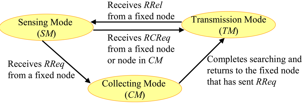
3.1.2. Mobile node
Sensing mode (SM)
Collecting mode (CM)
Transmission mode (TM)
3.2. Moving strategy of mobile nodes
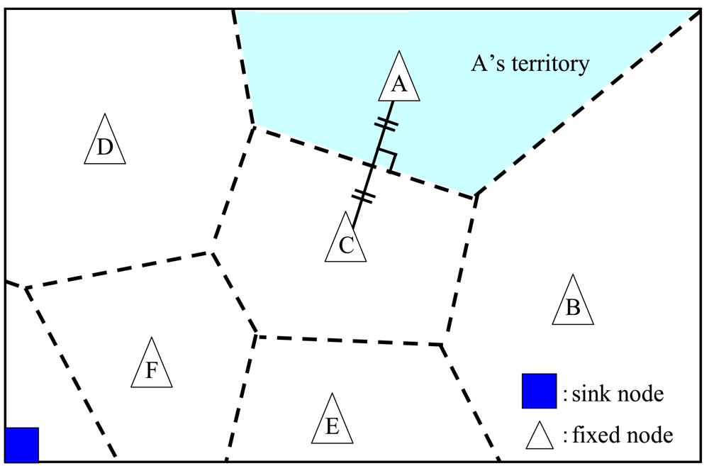
- It moves to connect to the nearest fixed node (i.e. the fixed node in the current territory) and transmits its acquired data.
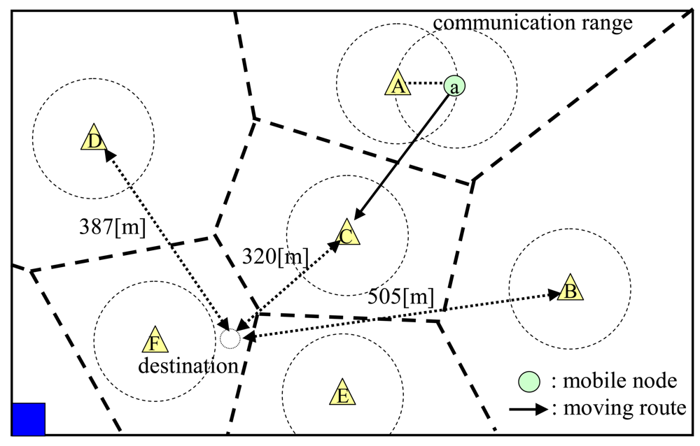
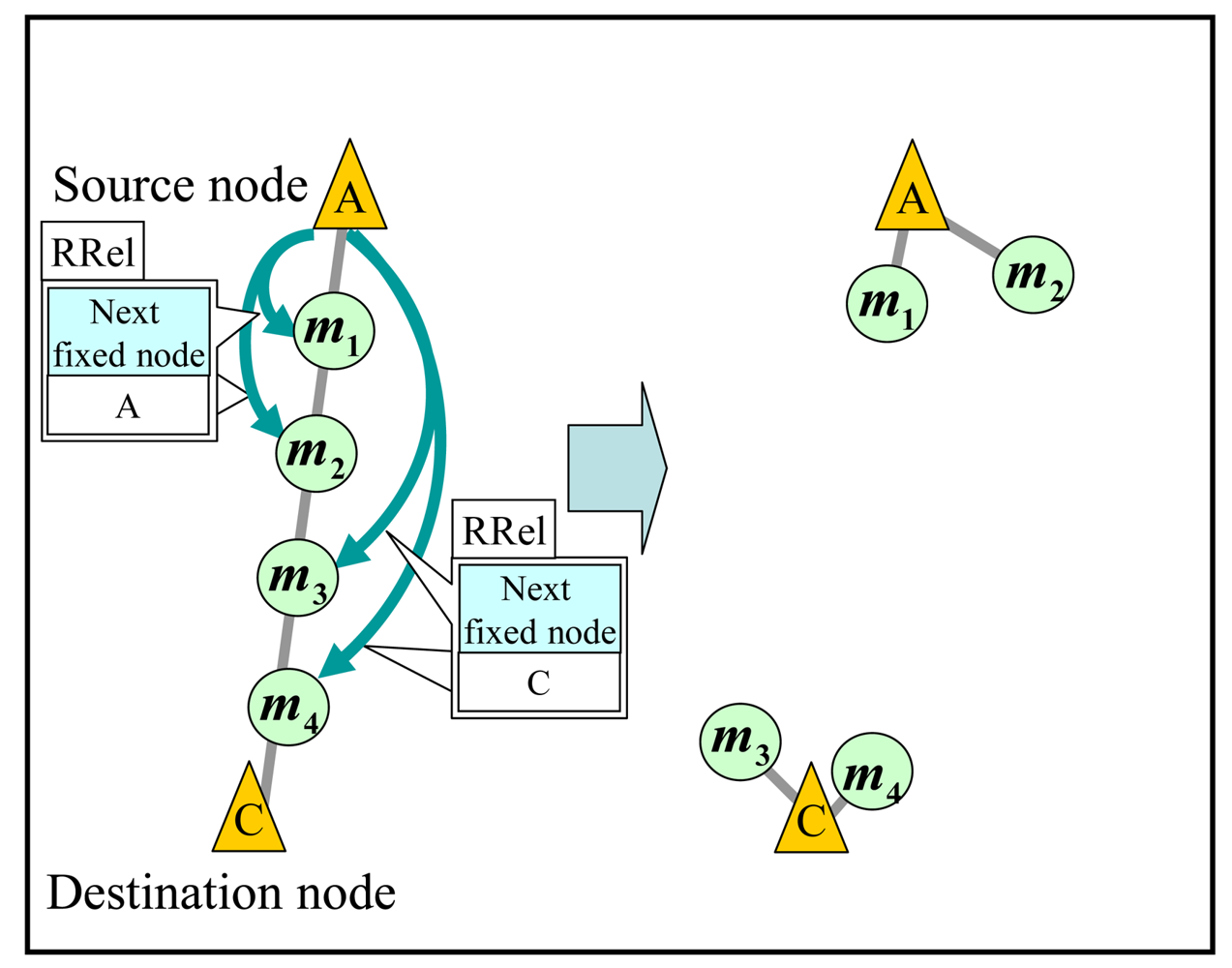
- It calculates the distances between its destination and all fixed nodes in the adjacent territories and moves to the fixed node that is the nearest to its destination. In addition, it sends information on its identifier, its next fixed node to move, and its destination to the connecting fixed node before moving to the next fixed node. Figure 3 shows an example to choose the next fixed node to move. After transmitting its acquired data to fixed node A, the mobile node a calculates the distances between its destination and fixed nodes B, C, and D, which are in territories adjacent to A's territory. After that, it chooses fixed node C that is the nearest to the destination and moves there. These procedures are repeated until the mobile node connects to the fixed node that has charge of the territory which contains the destination.
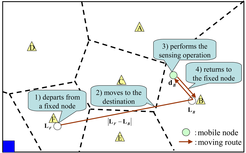
- It moves to its destination and does a sensing operation.
3.3. Data Transmission
3.3.1. Selection of the next fixed node
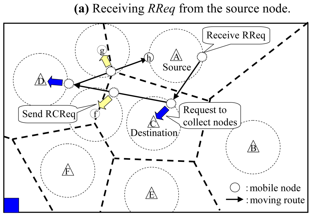
3.3.2. Request for collecting mobile nodes
- It calculates the number of mobile nodes which are performing a sensing operation in the territory of the connected fixed node. This can be done by checking the ‘next destination’ record in the information held by the fixed node. Specifically, when the ‘next destination’ is in the territory of the fixed node, the corresponding mobile node is performing the sensing operation in the territory.
- It decreases Nreq in the RReq by that calculated number of nodes. This is because the mobile nodes performing a sensing operation in a territory will connect to the fixed node in the territory after the sensing operation. As described later, those mobile nodes will receive RCReq from the fixed node, and move to the source node to help data transmission.
- It sends the updated RReq to the fixed node.
- It chooses the next fixed node to go. Specifically, it checks the ‘next fixed node’ record in the information held by the fixed node, and chooses one to which the largest number of mobile nodes have gone, and which it has not visited yet.
- The next fixed node to go cannot be found.
- Nreq in RReq becomes zero.
- The time limit has come.
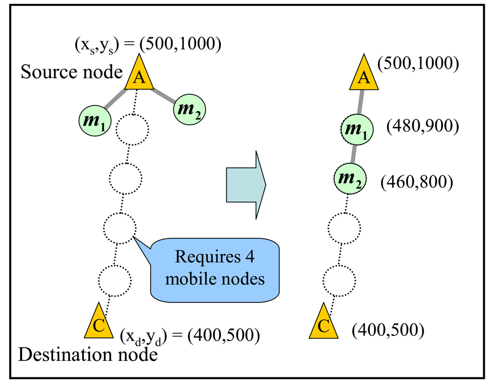
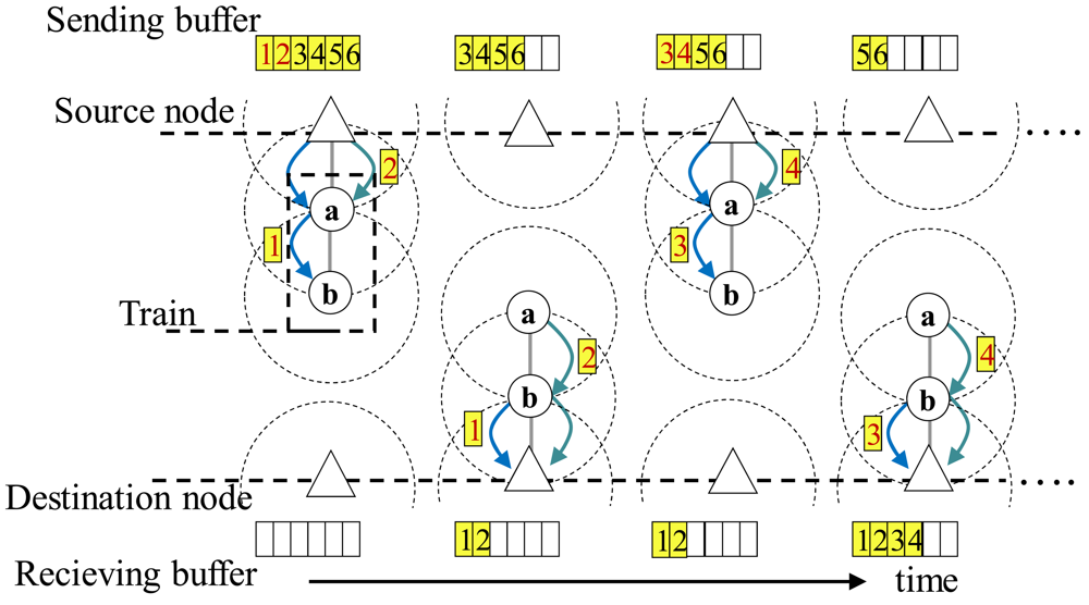
3.3.3 Data transmission using the collected node
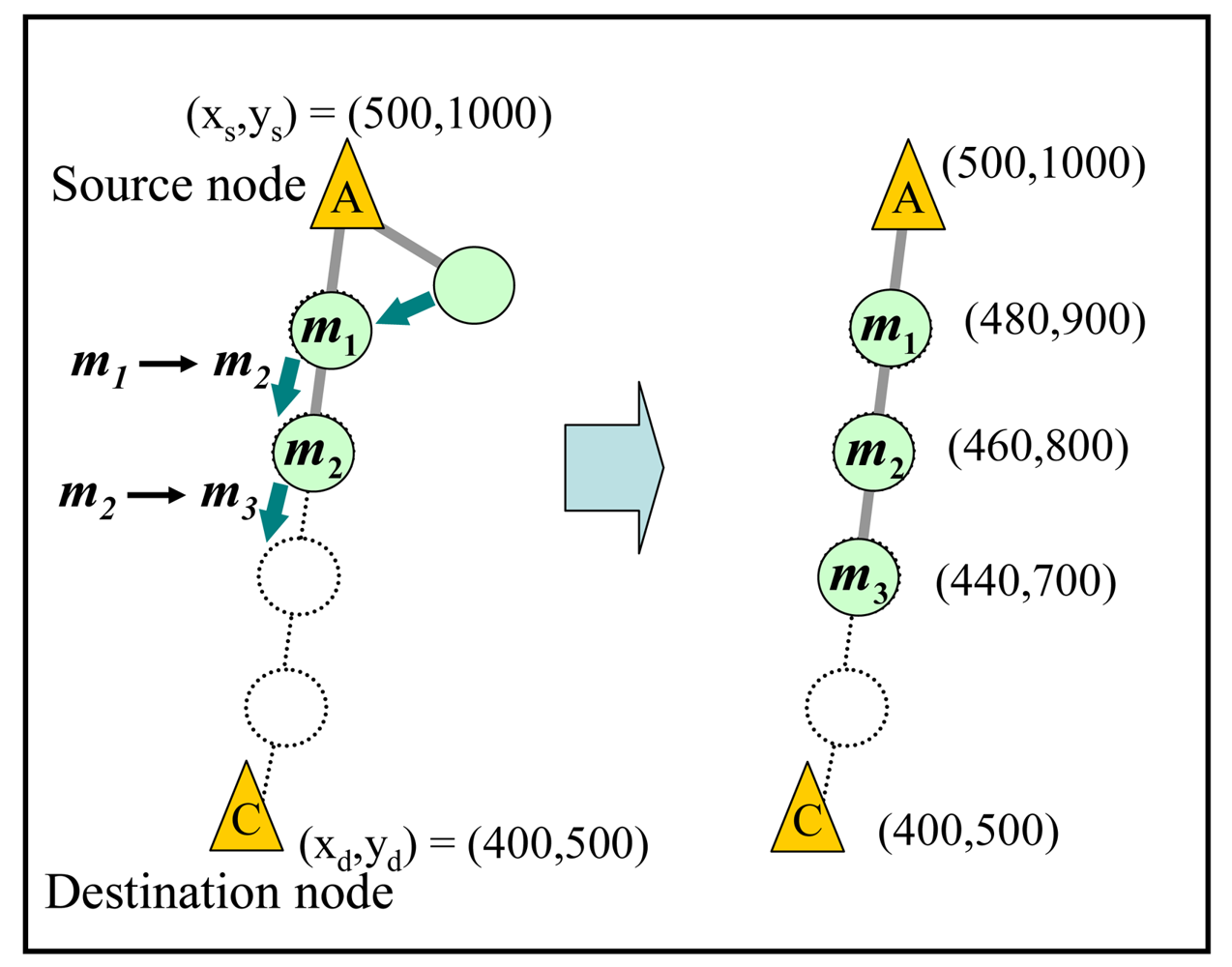
- The source node transmits a part of the accumulated data so that the amount of the transmitted data equals to the sum of memory spaces of the collected nodes.
- The collected nodes move toward the destination node with keeping same distances between adjacent nodes, and stop when the node at the other end of the line segment connects to the destination node.
- The collected nodes transmit all the data to the destination node through the line segment (communication route), and then, move back toward the source node.
3.3.4. Decision of the time limit
- Li: the location of fixed node i.
- Ti: the territory of fixed node i.
- di: the location of the destination (sensing point) of a mobile node in Ti (i.e. di ∈ Ti).
- Sarea: the size of the whole area (i.e. ).
- υm: the velocity of mobile nodes in SM.
- Tacq: the time for a sensing operation at a destination (sensing point).
- SF: the set of fixed nodes in the whole area.
- Nmov: the number of mobile nodes in the whole area.
- Nreqi: the required number of mobile nodes to construct the completed communication route from fixed node i.
3.4. Discussions
- The source node can collect mobile nodes easily since each mobile node travels around the fixed nodes as described in Subsection 3.2.
- Since each mobile node transmits the acquired data to the nearest fixed node, it can store new data more frequently.
- Since the accumulated data are transmitted by using multiple mobile nodes, the data can reach to the sink node easily even in a wide area.
- By applying train transmission, the source node can transmit the accumulated data even when the distance between the source and destination nodes is long.
4. Performance evaluation
4.1. Simulation environment
- ThroughputThe amount of data that arrive at the sink node per 1[sec].
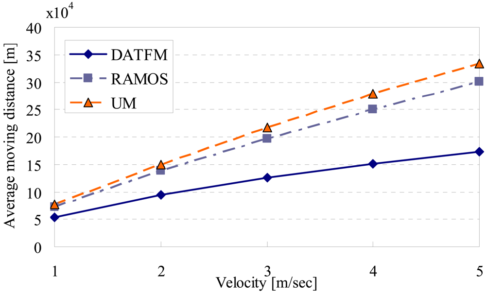
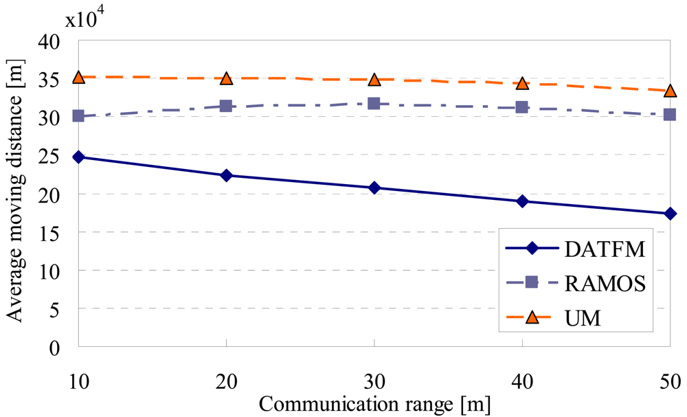
- Average moving distanceThe average of moving distances of all mobile nodes (i.e. all mobile nodes in DATFM, all nodes except those in category1 in RAMOS, and all nodes in UM) during the simulation period.
- Average delayThe average of the elapsed time after data are acquired until the data arrive at the sink node.
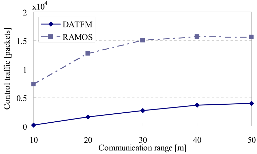
- Control trafficThe number of packets to control sensor nodes during the simulation period. Specifically, in DATFM, the total number of RReqs, RCReqs, and RRels sent by nodes becomes the control traffic. On the other hand, the control traffic in RAMOS is the total number of packets sent from nodes in
4.2. Effects of the velocity of node
4.2.1. Throughput
4.2.2. Average moving distance
4.2.3. Average delay
4.2.4. Control traffic
4.3. Effects of the communication range
4.3.1. Throughput
4.3.2. Average moving distance
4.3.3. Average delay
4.3.4. Control traffic
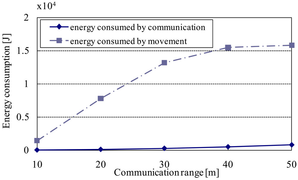
4.3.5. Energy consumption
4.4. Summary
5. Conclusions
Acknowledgments
References and Notes
- Cui, J.-H.; Kong, J.; Gerla, M.; Zhou, S. The challenges of building mobile underwater wireless networks for aquatic applications. IEEE Netw 2006, 20, 12–18. [Google Scholar]
- Roy, S.; Arabshahi, P.; Rouseff, D.; Fox, W.L.J. Wide area ocean networks: architecture and system design considerations. In Underwater Networks; ACM, 2006; pp. 25–32. [Google Scholar]
- Akyildiz, I.F.; Pompili, D.; Melodia, T. Underwater acoustic sensor networks: research challenges. Ad Hoc Netw. 2005, 3, 257–279. [Google Scholar]
- Lin, F.; Wang, Y.; Wu, H. Testbed implementation of delay/fault-tolerant mobile sensor network (dft-msn). In PerCom Workshops; IEEE Computer Society, 2006; pp. 321–327. [Google Scholar]
- Rao, R.N.; Kesidis, G. Purposeful mobility for relaying and surveillance in mobile ad hoc sensor networks. IEEE Trans. Mobile Comput. 2004, 3(3), 225–232. [Google Scholar]
- Wang, Y.; Wu, H. Delay/fault-tolerant mobile sensor network (dft-msn): A new paradigm for pervasive information gathering. IEEE Trans. Mobile Comput. 2007, 6(9), 1021–1034. [Google Scholar]
- Suzuki, R.; Makimura, K.; Saito, H.; Tobe, Y. Prototype of a sensor network with moving nodes. INSS 2004. [Google Scholar]
- Tobe, Y.; Suzuki, T. WISER: cooperative sensing using mobile robots. ICPADS 2005 2005, 388–392. [Google Scholar]
- Wang, K.-C.; Ramanathan, P. Collaborative sensing using sensors of uncoordinated mobility. In DCOSS, Lecture Notes in Computer Science; Springer, 2005; Volume 3560, pp. 293–306. [Google Scholar]
- Son, D.; Helmy, A.; Krishmacharl, B. The effect of mobility-induced location errors on geographic routing in mobile ad hoc and sensor networks:analysis and improvement using mobility prediction. IEEE Trans. Mobile Comput. 2004, 3(3), 233–245. [Google Scholar]
- Arboleda C, L.M.; Nasser, N. Cluster-based routing protocol for mobile sensor networks. International Conference on Quality of Service in Heterogeneous Wired/Wireless Networks, August 2006.
- Shinjo, T.; Ogawa, T.; Kitajima, S.; Hara, T.; Nishio, S. Mobile sensor control methods for reducing power consumption in sparse sensor network. SeNTIE 2008, 133–140. [Google Scholar]
- Lin, C.-Y.; Tseng, Y.-C. Structures for in-network moving object tracking in wireless sensor networks. In BROADNETS; IEEE Computer Society, 2004; pp. 718–727. [Google Scholar]
- Pompili, D.; Melodia, T.; Akyildiz, I.F. Routing algorithms for delay-insensitive and delay-sensitive applications in underwater sensor networks. In MOBICOM; ACM, 2006; pp. 298–309. [Google Scholar]
- Bahl, P.; Padmanabhan, V.N. Radar: An in-building rf-based user location and tracking system. INFOCOM 2000, 775–784. [Google Scholar]
- Hu, L.; Evans, D. Localization for mobile sensor networks. In MOBICOM; ACM, 2004; pp. 45–57. [Google Scholar]
- Goldenberd, D.K.; Lin, J.; Morse, A.S.; Rosen, B.E.; Yang, Y.R. Towards mobility as a network control primitive. In MOBIHOC; ACM, 2004; pp. 163–174. [Google Scholar]
- Rahimi, M.H.; Shah, H.; Sukhatme, G.S.; Heidemann, J.S.; Estrin, D. Studying the feasibility of energy harvesting in a mobile sensor network. In ICRA; IEEE, 2003; pp. 19–24. [Google Scholar]


| Node ID | Connected time | Next fixed node | Destination |
|---|---|---|---|
| a | 1,232 | E | (832,324) |
| c | 1,266 | F | (542,255) |
| f | 1,335 | E | (832,324) |
| i | 1,552 | C | (754,743) |
| o | 1,632 | C | (754,743) |
| Parameter | Value (Default) |
|---|---|
| Rcom | 10 ∼ 50 (50) |
| υm | 1.0 ∼ 5.0 (5.0) |
© 2009 by the authors; licensee Molecular Diversity Preservation International, Basel, Switzerland. This article is an open access article distributed under the terms and conditions of the Creative Commons Attribution license (http://creativecommons.org/licenses/by/3.0/).
Share and Cite
Treeprapin, K.; Kanzaki, A.; Hara, T.; Nishio, S. An Effective Mobile Sensor Control Method for Sparse Sensor Networks. Sensors 2009, 9, 327-354. https://doi.org/10.3390/s90100327
Treeprapin K, Kanzaki A, Hara T, Nishio S. An Effective Mobile Sensor Control Method for Sparse Sensor Networks. Sensors. 2009; 9(1):327-354. https://doi.org/10.3390/s90100327
Chicago/Turabian StyleTreeprapin, Kriengsak, Akimitsu Kanzaki, Takahiro Hara, and Shojiro Nishio. 2009. "An Effective Mobile Sensor Control Method for Sparse Sensor Networks" Sensors 9, no. 1: 327-354. https://doi.org/10.3390/s90100327