Chemical Characterization of Dew Water Collected in Different Geographic Regions of Poland

Abstract
:1. Introduction
2. Experimental Section
3. Results and Discussion
3.1. Chemical composition of dew
3.2. Correlation between concentrations
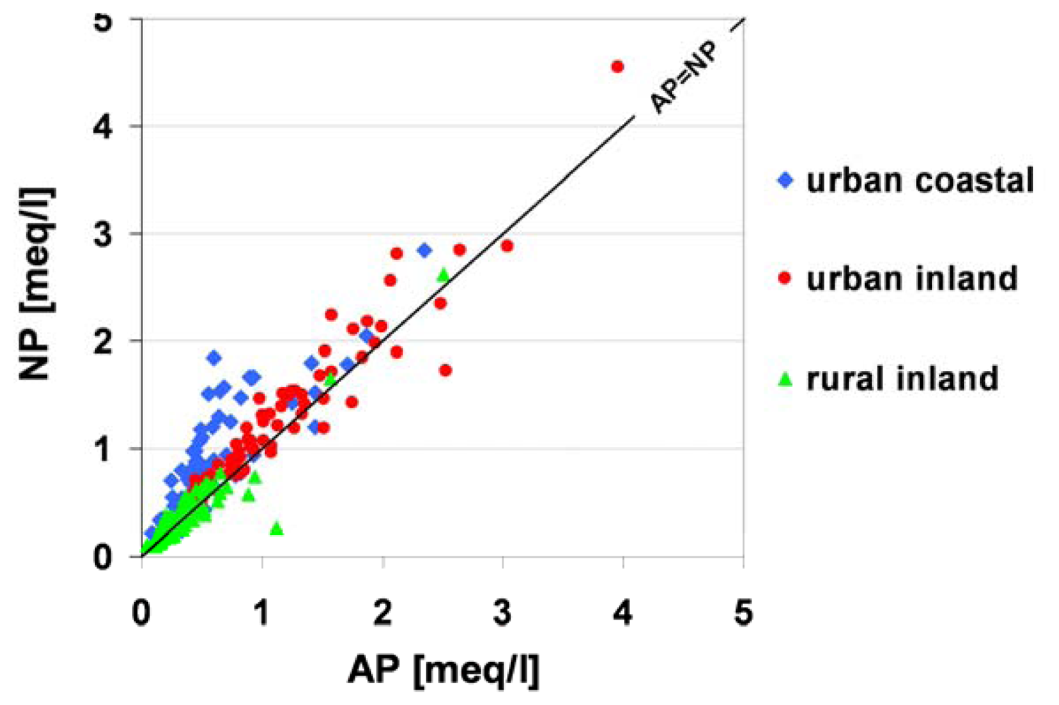
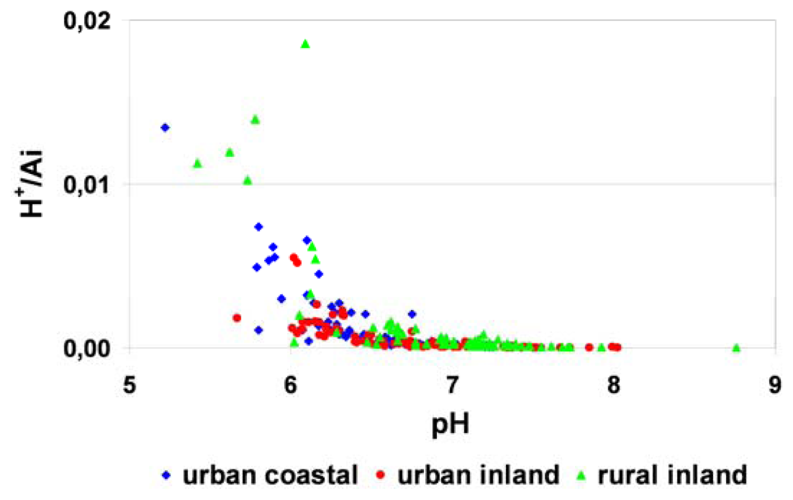
3.3. The dew acidification process
3.4. Ionic correlations between determined concentrations of analytes
3.5. Dew chemistry in relation to meteorological data
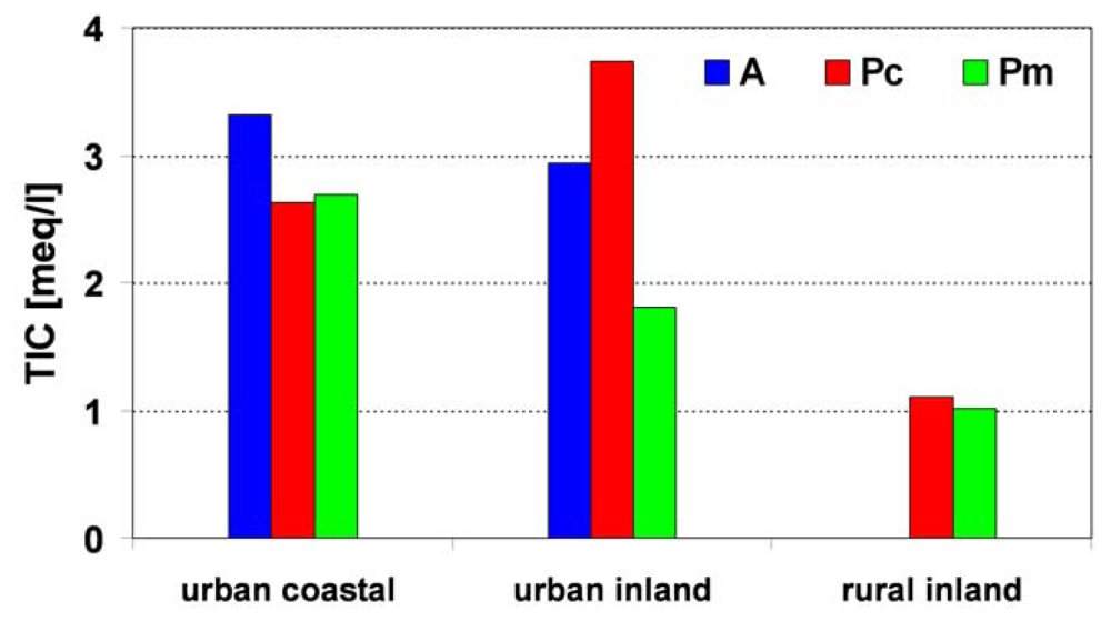
3.5.1. Type of air mass
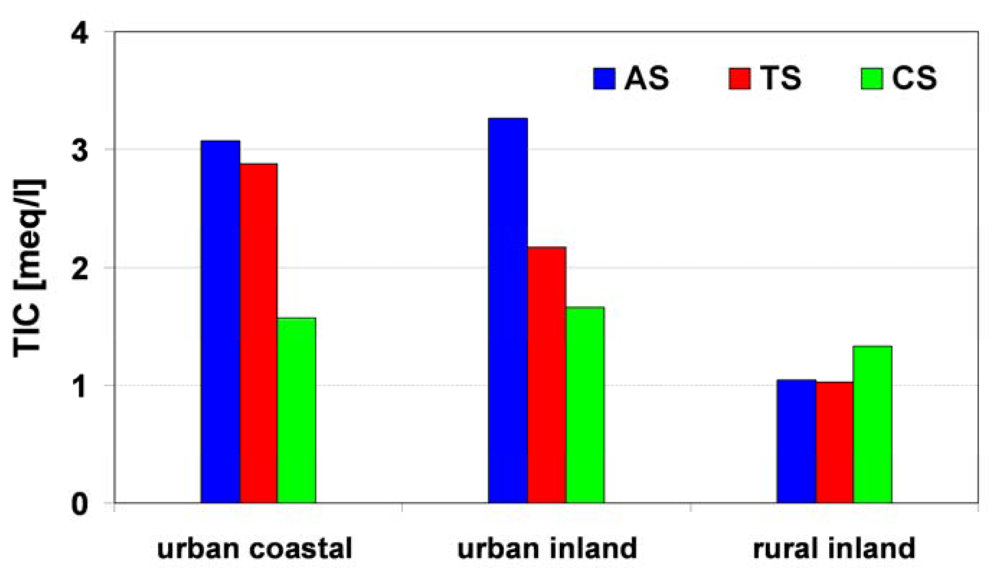
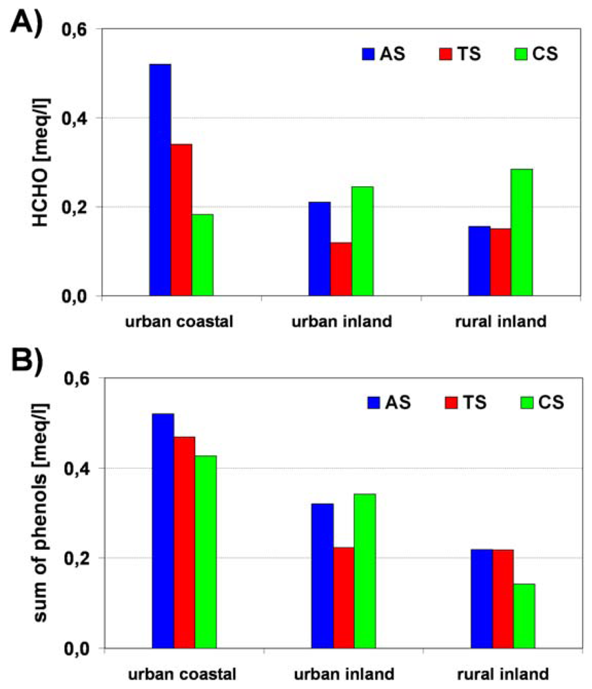
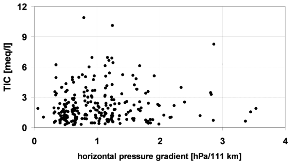
3.5.2. Synoptic situation
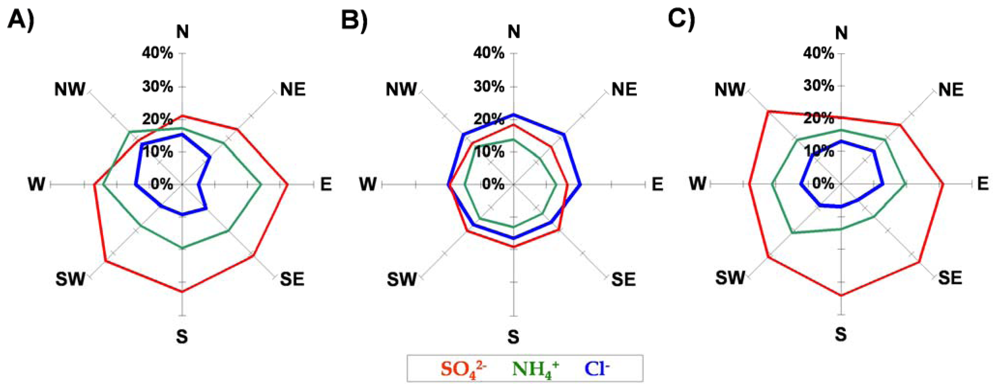
3.5.3. Direction of atmospheric circulation
4. Conclusions
Acknowledgments
References
- Taylor, R.C. (Ed.) Glossary of Meteorology; American Meteorological Society website visited 6 March 2007. (http://amsglossary.allenpress.com/glossary).
- Beysens, D. The formation of dew. Atmos. Res. 1995, 39, 215–237. [Google Scholar]
- Olszewski, J.L. Dew at various heights above ground. Ekol. Pol. 1976, 24, 639–668. [Google Scholar]
- Hutorowicz, H. Dew measurements at Olsztyn. Assoc. Int. Hydrol. Scient. 1963, 65, 352–359. [Google Scholar]
- Monteith, J.L. Dew: facts and fallacies. In The water relations of plants; Rutter, A.J., Whitehead, F.H., Eds.; Wiley: New York, 1963; pp. 37–56. [Google Scholar]
- Garratt, J.R.; Segal, M. On the contribution of atmospheric moisture to dew formation. Bound. Layer Meteor 1988, 45, 209–236. [Google Scholar]
- Richards, K. Hardware scale modeling of summertime patterns of urban dew and surface moisture in Vancouver, BC, Canada. Atmos. Res. 2002, 64, 313–321. [Google Scholar]
- Jacobs, A.F.G.; Heusinkveld, B.G.; Berkiwicz, S.M. Dew deposition and drying in a desert system: a simple simulation model. J. Arid Environ. 1999, 42, 211–222. [Google Scholar]
- Jacobs, A.F.G.; Heusinkveld, B.G.; Berkiwicz, S.M. Force-restore technique for ground surface temperature and moisture content in dry desert system. Water Resour. Res. 2000, 36, 1261–1268. [Google Scholar]
- Jacobs, A.F.G.; Heusinkveld, B.G.; Berkiwicz, S.M. A simple model for potential dewfall in an arid region. Atmos. Environ. 2002, 64, 285–295. [Google Scholar]
- Evenari, M.; Shanan, L.; Tadmor, N. The Negev: Challenge of a Desert, 2nd Ed. ed; Harvard Univ. Press: Cambridge, MA, 1982. [Google Scholar]
- Richards, K. Observation and modeling of urban dew. PhD thesis, University of British Columbia, Vancouver, Canada, 1999. [Google Scholar]
- Grimmond, C.S.B.; Oke, T.R. Variability of evapotranspiration rates in urban areas. In Biometeorology and Urban Climatology at the Turn of the Millennium, Selected papers from the ICB-ICU'99 Conference, Geneva; de Dear, R.J., Kalma, J.D., Oke, T.R., Auliciems, A., Eds.; 2000; pp. 475–480. [Google Scholar]
- Beysens, D.; Ohayon, C.; Muselli, M.; Clus, O. Chemical and biological characteristics of dew and rain water in an urban coastal area (Bordeaux, France). Atmos. Environ. 2006, 40, 3710–3723. [Google Scholar]
- Beysens, D.; Muselli, M.; Milimouk, I.; Ohayon, C.; Berkowicz, S. M.; Soyeux, E.; Mileta, M.; Ortega, P. Application of passive radiative cooling for dew condensation. Energy 2006, 31, 1967–1979. [Google Scholar]
- Muselli, M.; Beysens, D.; Marcillat, J.; Milimouk, I.; Nilsson, T.; Louche, A. Dew water collector for potable water in Ajaccio. Atmos. Res. 2002, 64, 297–312. [Google Scholar]
- Zuo, Y.; Wang, C.; Van, T. Simultaneous determination of nitrite and nitrate in dew, rain, snow and lake water samples by ion-pair high-performance liquid chromatography. Talanta 2006, 70, 281–285. [Google Scholar]
- Rubio, M. A.; Guerrero, M. J.; Villena, G.; Lissi, E. Hydroperoxides in dew water in downtown Santiago, Chile. A comparison with gas-phase values. Atmos. Environ. 2006, 40, 6165–6172. [Google Scholar]
- Jiries, A. Chemical composition of dew in Amman, Japan. Atmos. Res. 2001, 57, 261–268. [Google Scholar]
- Polkowska, Ż.; Astel, A.; Walna, B.; Małek, S.; Mędrzycka, K.; Górecki, T.; Siepak, J.; Namieśnik, J. Chemometric analysis of rainwater and throughfall at several sites in Poland. Atmos. Environ. 2005, 39, 837–855. [Google Scholar]
- Cardenas, L.M.; Brassington, D.J.; Allan, B.J.; Coe, H.; Alicke, B.; Platt, U.; Wilson, K.M.; Plane, J.M.C.; Penkett, S.A. Intercomparison of formaldehyde measurements in clean and polluted atmospheres. J. Atmos. Chem. 2000, 37, 53–80. [Google Scholar]
- Cini, R.; Prodi, F.; Santachiara, G.; Porcu., F.; Bellandi, S.; Stortini, A.M.; Oppo, C.; Udisti, R.; Pantani, F. Chemical characterization of cloud episodes at a ridge in Tuscan Appenines, Italy. Atmos. Res. 2002, 61, 311–334. [Google Scholar]
- Zimmermann, F.; Matschullat, J.; Bruggemann, E.; Pleβow, K.; Wienhaus, O. Temporal and elevation-related variability in precipitation chemistry from 1993 to 2002, Eastern Erzgebirge, Germany. Water, Air, Soil Pollut. 2006, 170, 123–141. [Google Scholar]
- Möller, D.; Acker, K.; Wieprecht, W. A relationship between liquid water content and chemical composition in clouds. Atmos. Res. 1996, 41, 321–335. [Google Scholar]
- Watanabe, K.; Ishizaka, Y.; Takenaka, C. Chemical characteristics of cloud water over the Japan Sea and the North western Pacific Ocean near the central part of Japan: airborne measurements. Atmos. Environ. 2001, 35, 645–655. [Google Scholar]
- Hara, H.; Kitamura, M.; Mori, A.; Noguchi, I.; Ohizumi, T.; Seto, S.; Takeuchi, T.; Deguchi, T. Precipitation chemistry in Japan 1989-1993. Water Air Soil Pollut. 1995, 85, 2307–2312. [Google Scholar]
- Watanabe, K.; Takebe, Y.; Sode, N.; Igarashi, Y.; Takahashi, H.; Dokiya, Y. Fog and rain water chemistry at Mt. Fuji: A case study during the September 2002 campaign. Atmos. Res. 2006, 82, 652–662. [Google Scholar]
- Błaś, M.; Sobik, M.; Quiel, F.; Netzel, P. Temporal and spatial variations of fog in the Western Sudety Mts., Poland. Atmos. Res. 2002, 64, 19–28. [Google Scholar]
- Dore, A.J.; Sobik, M.; Migała, K. Patterns of precipitation and pollutant deposition in the western Sudete Mountains. Atmos. Environ. 1999, 33, 3301–3312. [Google Scholar]
- Sasakawa, M.; Uematsu, M. Relative contribution of chemical composition to acidification of sea fog (stratus) over the northern North Pacific and its marginal seas. Atmos. Environ. 2005, 39, 1357–1362. [Google Scholar]
- Daily Synoptic Bulletin; IMGW: Warszawa, 2006.


| Sampling site location | Geographic coordinates | Elevation [m a.s.l.] | Type of area | Landform type | Site description |
|---|---|---|---|---|---|
| Coastal urban sites | |||||
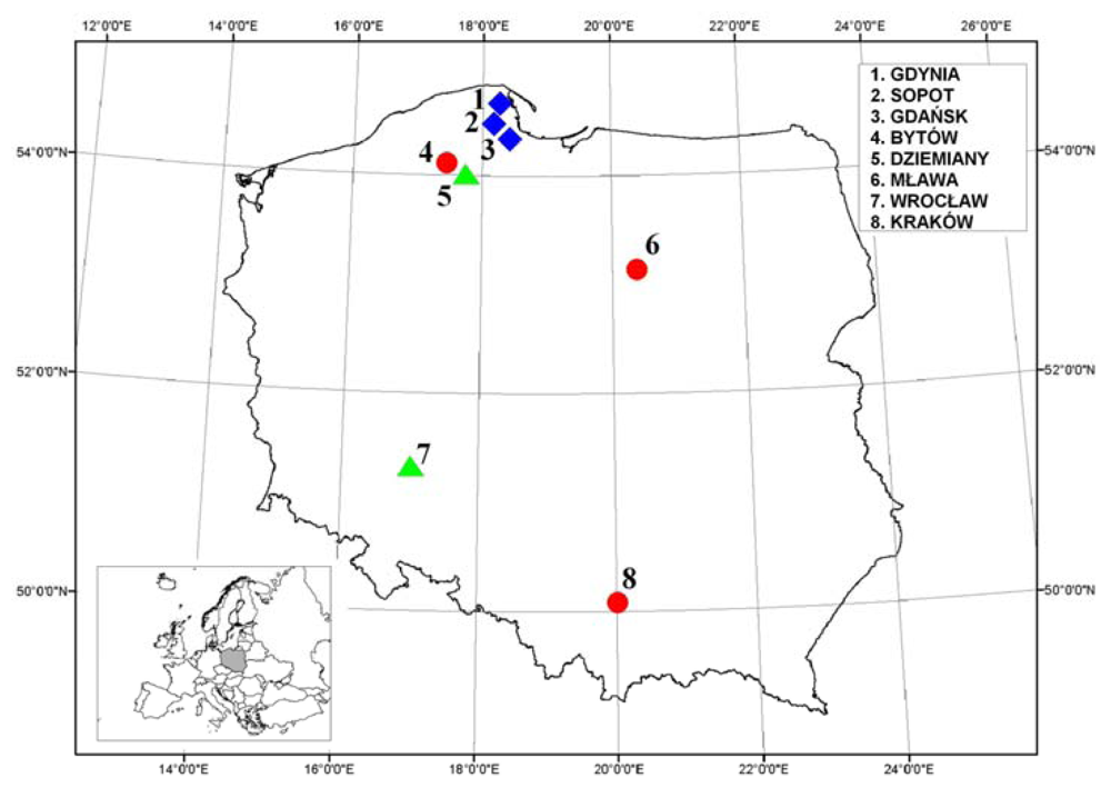
| Gdańsk | 54° 20″ N 18° 36″ E | 74 | suburban | gentle slope | 200 m away from the main road connecting the Gdańsk centre with the Tricity ring road; 3 km WSW of the Gdańsk city centre and 8 km away from the Gdańsk Gulf; 460,000 citizens |
| Sopot | 54° 27″ N 18° 34″ E | 5 | urban | flat | intersection close to the city centre; in the vicinity of the coast line (200 m), surrounded directly by allotments and a residential area; 40,500 citizens |
| Gdynia | 54° 29″ N 18° 32″ E | 37 | urban | flat | intersection close to the city centre with very intensive road transport; close to the coast line (1.5 km), surrounded by a residential area; 253,500 citizens |
| Inland urban sites | |||||
| Mława | 53° 08″ N 20° 21″ E | 142 | urban | flat | outskirts of the country town; sampling point located in the vicinity of the allotments and a building with flats; 30,000 citizens |
| Kraków | 50° 07″ N 19° 55″ E | 225 | suburban | flat | sampling point surrounded by allotments and a building with flats; 757,500 citizens |
| Bytów | 54° 10″ N 17° 30″ E | 147 | urban | flat | outskirts of the city centre; only single-family buildings; 23,500 citizens |
| Rural sites | |||||
| Dziemiany | 54° 00″ N 17° 46″ E | 166 | rural, lake district and foresty | hilly | village located on the outskirts of the Wdzyński Landscape Park; surrounded by a forest; 1,600 citizens |
| Wrocław | 51° 07″ N 17° 05″ E | 116 | rural | Flat (mikro concave) | Meteorological Observatory; measuring site situated on the east of Wrocław, 5 km from the centre; located close to the Odra river and Szczytnicki park, surrounded directly by allotments |
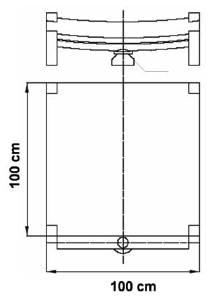
| Characteristics of the sampler | Size of the sampler |
|---|---|
| 100 cm × 100 cm (Figure 2) |
| |
|
| Analyte | Technique | Analytical parameters | Limit of detection [mg/L] | Precision [% RSD] |
|---|---|---|---|---|
| Anions | IC | AS9-HC column (2 × 250 mm), | Br-, F-, Cl-, | 1 |
| AutoSuppression Recycle Mode | NO3-, SO42-= 0.01 | |||
| ASRC®-ULTRA (2 mm), conductivity | NO2-=0.05 | |||
| detection, eluent 9.0 mM Na2CO3, | PO43-= 0.04 | |||
| flow rate 0.25 ml/min | ||||
| Cations | CS12A column (2 × 250 mm), | 0.01 | ||
| AutoSuppression Recycle Mode CSRS | ||||
| ®-ULTRA (2 mm), conductivity | ||||
| detection, eluent 20 mM | ||||
| Methanesulfonic Acid, | ||||
| flow rate 0.25 ml/min | ||||
| Phenols | photometry | Absorbance measured at 495 nm | 0.001 | 5 |
| HCHO | Absorbance measured at 585 nm | 0.005 | 5 |
| ANALYTES | STATS | URBAN COASTAL | URBAN INLAND | RURAL INLAND | ||||||
|---|---|---|---|---|---|---|---|---|---|---|
| Gdańsk | Gdynia | Sopot | Bytów | Kraków | Mława | Dziemiany | Wrocław | |||
| 1 | 2 | 3 | 4 | 5 | 6 | 7 | 8 | 10 | 11 | |
| N | 13 | 31 | 20 | 36 | 19 | 29 | 33 | 53 | ||
| Conductivity | max | 288 | 482 | 747 | 518 | 881 | 298 | 276 | 396 | |
| mean | 151 | 151 | 183 | 171 | 337 | 152 | 92. 0 | 56.7 | ||
| min | 28.8 | 31.2 | 35.1 | 29.2 | 56.2 | 69.5 | 19.2 | 20.2 | ||
| f (%) | 100 | 100 | 100 | 100 | 100 | 100 | 100 | 100 | ||
| pH | max | 7.20 | 7.35 | 7.03 | 7.99 | 8.02 | 7.32 | 8.76 | 7.47 | |
| mean | 6.31 | 6.52 | 6.55 | 6.80 | 7.12 | 6.49 | 7.15 | 6.63 | ||
| min | 5.22 | 5.80 | 5.94 | 6.01 | 6.57 | 5.67 | 5.62 | 4.16 | ||
| f (%) | 100 | 100 | 100 | 100 | 100 | 100 | 100 | 100 | ||
| Na+ | max | 0.88 | 1.07 | 0.26 | 0.68 | 0.22 | 0.34 | 0.96 | 0.22 | |
| mean | 0.34 | 0.34 | 0.13 | 0.15 | 0.11 | 0.14 | 0.11 | 0.043 | ||
| min | 0.013 | 0.024 | 0.034 | 0.020 | 0.040 | 0.0030 | 0.026 | 0.0052 | ||
| f (%) | 100 | 100 | 100 | 100 | 100 | 100 | 100 | 100 | ||
| NH4+ | max | 0.45 | 1.18 | 0.42 | 0.60 | 0.59 | 0.70 | 0.84 | 0.82 | |
| mean | 0.25 | 0.23 | 0.27 | 0.33 | 0.29 | 0.35 | 0.26 | 0.15 | ||
| min | 0.063 | 0.029 | 0.085 | 0.15 | 0.067 | 0.10 | 0.084 | 0.039 | ||
| f (%) | 100 | 35.5 | 100 | 100 | 100 | 100 | 100 | 100 | ||
| K+ | max | 0.37 | 0.43 | 0.17 | 0.26 | 0.36 | 0.22 | 0.17 | 0.16 | |
| mean | 0.15 | 0.13 | 0.092 | 0.077 | 0.12 | 0.086 | 0.052 | 0.046 | ||
| min | 0.029 | 0.0095 | 0.037 | 0.025 | 0.064 | 0.019 | 0.018 | 0.0067 | ||
| f (%) | 100 | 100 | 100 | 100 | 100 | 100 | 100 | 100 | ||
| Mg2+ | max | 0.45 | 0.77 | 0.32 | 0.62 | 1.14 | 0.46 | 0.15 | 0.18 | |
| mean | 0.23 | 0.21 | 0.072 | 0.074 | 0.29 | 0.093 | 0.028 | 0.031 | ||
| min | 0.026 | 0.032 | 0.012 | 0.0025 | 0.012 | 0.011 | 0.0025 | 0.00083 | ||
| f (%) | 100 | 100 | 100 | 100 | 100 | 100 | 100 | 100 | ||
| Ca2+ | max | 1.81 | 2.49 | 1.40 | 2.80 | 4.43 | 2.16 | 1.78 | 0.84 | |
| mean | 0.89 | 0.74 | 0.75 | 0.73 | 1.33 | 0.68 | 0.27 | 0.16 | ||
| min | 0.13 | 0.086 | 0.15 | 0.037 | 0.15 | 0.16 | 0.027 | 0.030 | ||
| f (%) | 100 | 100 | 100 | 100 | 100 | 100 | 100 | 100 | ||
| F- | max | 0.10 | 0.056 | 0.020 | 0.042 | 0.039 | 0.062 | 0.22 | 0.25 | |
| mean | 0.018 | 0.012 | 0.010 | 0.016 | 0.021 | 0.011 | 0.036 | 0.015 | ||
| min | 0.0016 | 0.0016 | 0.0016 | 0.00053 | 0.0042 | 0.0016 | 0.0042 | 0.00053 | ||
| f (%) | 76.9 | 71.0 | 100 | 94.6 | 100 | 100 | 100 | 83.0 | ||
| Cl- | max | 1.14 | 1.71 | 1.00 | 0.97 | 0.84 | 0.77 | 0.23 | 0.34 | |
| mean | 0.45 | 0.55 | 0.54 | 0.20 | 0.23 | 0.26 | 0.13 | 0.067 | ||
| min | 0.065 | 0.062 | 0.27 | 0.027 | 0.052 | 0.059 | 0.065 | 0.0037 | ||
| f (%) | 100 | 100 | 100 | 100 | 100 | 100 | 100 | 100 | ||
| NO2- | max | 0.070 | 0.21 | 0.052 | 0.31 | 0.16 | 0.049 | 0.13 | 0.048 | |
| mean | 0.030 | 0.035 | 0.028 | 0.054 | 0.052 | 0.023 | 0.012 | 0.014 | ||
| min | 0.0041 | 0.0035 | 0.0048 | 0.0024 | 0.0072 | 0.0071 | 0.0015 | 0.0028 | ||
| f (%) | 76.9 | 67.7 | 55.0 | 86.5 | 47.4 | 51.7 | 81.8 | 100 | ||
| NO3- | max | 0.72 | 0.47 | 0.54 | 0.81 | 0.34 | 0.51 | 1.74 | 0.50 | |
| mean | 0.16 | 0.12 | 0.12 | 0.15 | 0.12 | 0.18 | 0.12 | 0.062 | ||
| min | 0.0066 | 0.026 | 0.032 | 0.00097 | 0.0082 | 0.012 | 0.013 | 0.015 | ||
| f (%) | 100 | 100 | 100 | 100 | 94.7 | 96.6 | 100 | 100 | ||
| PO43- | max | 0.40 | 0.47 | 0.090 | 0.057 | 0.12 | 0.13 | 0.24 | 0.12 | |
| mean | 0.092 | 0.10 | 0.031 | 0.020 | 0.049 | 0.044 | 0.034 | 0.019 | ||
| min | 0.0091 | 0.0044 | 0.0073 | 0.0075 | 0.0059 | 0.012 | 0.0047 | 0.0028 | ||
| f (%) | 61.5 | 74.2 | 75.0 | 35.1 | 63.2 | 69.0 | 51.5 | 26.4 | ||
| SO42- | max | 1.40 | 1.94 | 0.87 | 4.46 | 3.77 | 1.71 | 1.22 | 1.07 | |
| mean | 0.72 | 0.48 | 0.40 | 0.95 | 1.37 | 0.68 | 0.40 | 0.25 | ||
| min | 0.067 | 0.030 | 0.15 | 0.11 | 0.34 | 0.30 | 0.030 | 0.065 | ||
| f (%) | 100 | 100 | 100 | 100 | 100 | 100 | 100 | 100 | ||
| SO42- + NO3- | max | 1.91 | 2.41 | 0.95 | 5.10 | 3.98 | 2.16 | 2.51 | 1.58 | |
| mean | 0.88 | 0.60 | 0.52 | 1.10 | 1.49 | 0.85 | 0.52 | 0.31 | ||
| min | 0.12 | 0.091 | 0.19 | 0.18 | 0.38 | 0.42 | 0.048 | 0.082 | ||
| Cl- / Na+ | max | 8.42 | 6.55 | 10.9 | 4.18 | 3.91 | 57.6 | 4.63 | 7.02 | |
| mean | 2.29 | 2.48 | 4.92 | 1.64 | 1.98 | 3.88 | 2.15 | 1.86 | ||
| min | 0.32 | 0.80 | 1.68 | 0.21 | 0.83 | 0.67 | 0.086 | 0.059 | ||
| SO42- / Na+ | max | 17.3 | 8.61 | 8.55 | 14.6 | 29.0 | 287 | 14.5 | 24.5 | |
| mean | 3.94 | 2.56 | 3.64 | 6.72 | 13.7 | 15.0 | 5.99 | 7.20 | ||
| min | 1.04 | 0.25 | 0.93 | 1.56 | 5.52 | 1.48 | 0.91 | 2.18 | ||
| K+ / Na+ | max | 4.12 | 3.81 | 1.16 | 1.45 | 3.44 | 6.23 | 2.86 | 2.50 | |
| mean | 1.01 | 0.70 | 0.77 | 0.68 | 1.35 | 0.83 | 0.75 | 1.21 | ||
| min | 0.065 | 0.13 | 0.52 | 0.14 | 0.49 | 0.26 | 0.093 | 0.30 | ||
| Ca2+ / Na+ | max | 16.5 | 14.4 | 18.8 | 12.3 | 24.1 | 279 | 17.6 | 30.5 | |
| mean | 4.57 | 4.45 | 6.65 | 4.81 | 12.5 | 14.4 | 4.38 | 5.41 | ||
| min | 1.01 | 0.55 | 1.36 | 0.75 | 2.42 | 2.12 | 0.12 | 0.87 | ||
| Mg2+ / Na+ | max | 8.99 | 2.37 | 2.36 | 1.52 | 6.53 | 40.5 | 1.27 | 2.08 | |
| mean | 1.54 | 0.88 | 0.63 | 0.40 | 2.66 | 1.97 | 0.33 | 0.70 | ||
| min | 0.090 | 0.20 | 0.12 | 0.086 | 0.19 | 0.14 | 0.048 | 0.033 | ||
| NO3- / SO42- | max | 0.83 | 2.08 | 2.95 | 0.86 | 0.30 | 1.67 | 2.25 | 0.88 | |
| mean | 0.27 | 0.39 | 0.39 | 0.24 | 0.099 | 0.33 | 0.26 | 0.27 | ||
| min | 0.029 | 0.086 | 0.069 | 0.0024 | 0.013 | 0.022 | 0.013 | 0.068 | ||
| Ca2+ + NH4+ / NO3- + SO42- | max | 1.72 | 2.84 | 2.77 | 1.44 | 1.31 | 1.54 | 2.34 | 1.72 | |
| mean | 1.03 | 1.45 | 2.00 | 1.09 | 1.08 | 1.21 | 1.17 | 1.03 | ||
| min | 0.69 | 0.84 | 1.31 | 0.64 | 0.93 | 0.94 | 0.24 | 0.65 | ||
| Σ anions / Σ cations | max | 0.99 | 0.99 | 1.39 | 1.21 | 0.94 | 1.06 | 1.28 | 1.31 | |
| mean | 0.86 | 0.85 | 0.87 | 0.97 | 0.85 | 0.87 | 0.97 | 0.99 | ||
| min | 0.80 | 0.80 | 0.80 | 0.88 | 0.80 | 0.80 | 0.86 | 0.85 | ||
| TIC | max | 6.13 | 8.24 | 3.77 | 10.1 | 10.9 | 6.87 | 6.20 | 3.79 | |
| mean | 3.08 | 2.77 | 2.43 | 2.73 | 3.93 | 2.51 | 1.43 | 0.83 | ||
| min | 0.39 | 0.62 | 0.88 | 0.52 | 0.97 | 1.18 | 0.32 | 0.27 | ||
| PDI [% ] | max | 11.1 | 11.1 | 16.3 | 9.51 | 10.8 | 11.1 | 12.4 | 13.4 | |
| mean | 7.48 | 8.13 | 9.11 | 4.12 | 8.18 | 7.15 | 4.43 | 4.25 | ||
| min | 0.65 | 0.49 | 0.84 | 0.019 | 2.84 | 0.19 | 0.22 | 0.34 | ||
| pAi | max | 3.92 | 4.07 | 3.74 | 3.76 | 3.42 | 3.38 | 4.36 | 4.10 | |
| mean | 3.19 | 3.37 | 3.33 | 3.15 | 2.88 | 3.11 | 3.39 | 3.60 | ||
| min | 2.73 | 2.63 | 3.03 | 2.30 | 2.40 | 2.67 | 2.60 | 2.81 | ||
| AP | max | 1.86 | 2.34 | 0.93 | 5.05 | 3.95 | 2.12 | 2.50 | 1.56 | |
| mean | 0.84 | 0.56 | 0.50 | 1.08 | 1.47 | 0.83 | 0.50 | 0.30 | ||
| min | 0.12 | 0.086 | 0.18 | 0.17 | 0.38 | 0.42 | 0.044 | 0.079 | ||
| NP | max | 2.05 | 2.85 | 1.67 | 3.26 | 4.54 | 2.81 | 2.62 | 1.65 | |
| mean | 0.93 | 0.81 | 1.02 | 1.06 | 1.61 | 1.03 | 0.53 | 0.31 | ||
| min | 0.13 | 0.19 | 0.28 | 0.22 | 0.37 | 0.46 | 0.11 | 0.090 | ||
| NP / AP | max | 1.83 | 3.09 | 2.88 | 1.46 | 1.32 | 1.59 | 2.51 | 1.73 | |
| mean | 1.07 | 1.55 | 2.05 | 1.11 | 1.08 | 1.23 | 1.19 | 1.05 | ||
| min | 0.71 | 0.86 | 1.34 | 0.65 | 0.93 | 0.95 | 0.23 | 0.65 | ||
| loss Mg2+ | max | 0.017 | 0.019 | 0.0069 | 0.17 | 0.011 | ||||
| mean | 0.062 | 0.014 | 0.011 | 0.0045 | 0.0026 | 0.0037 | 0.023 | 0.0049 | ||
| min | 0.0023 | 0.00027 | 0.0015 | 0.00037 | 0.0018 | |||||
| nss SO42- | max | 1.38 | 1.87 | 0.85 | 4.41 | 3.74 | 1.67 | 1.11 | 1.06 | |
| mean | 0.67 | 0.44 | 0.39 | 0.93 | 1.36 | 0.66 | 0.38 | 0.24 | ||
| min | 0.065 | 0.024 | 0.14 | 0.11 | 0.34 | 0.28 | 0.026 | 0.062 | ||
| nss Ca2+ | max | 1.80 | 2.46 | 1.39 | 2.78 | 4.42 | 2.14 | 1.77 | 0.84 | |
| mean | 0.87 | 0.73 | 0.75 | 0.73 | 1.32 | 0.67 | 0.27 | 0.16 | ||
| min | 0.13 | 0.082 | 0.15 | 0.036 | 0.15 | 0.15 | 0.026 | 0.029 | ||
| loss Mg2+/ Mg2+ | max | 0.89 | 1.67 | 0.69 | 3.81 | 5.96 | ||||
| mean | 1.55 | 0.14 | 0.57 | 0.49 | 0.23 | 0.29 | 1.07 | 1.77 | ||
| min | 0.052 | 0.040 | 0.080 | 0.034 | 0.23 | |||||
| nss SO42- SO42- | max | 0.99 | 0.99 | 0.99 | 0.99 | 1.00 | 1.00 | 0.99 | 1.00 | |
| mean | 0.94 | 0.90 | 0.95 | 0.97 | 0.99 | 0.97 | 0.97 | 0.98 | ||
| min | 0.88 | 0.52 | 0.87 | 0.92 | 0.98 | 0.92 | 0.87 | 0.94 | ||
| nss Ca2+ / Ca2+ | max | 1.00 | 1.00 | 1.00 | 1.00 | 1.00 | 1.00 | 1.00 | 1.00 | |
| mean | 0.98 | 0.98 | 0.99 | 0.98 | 0.99 | 0.99 | 0.97 | 0.99 | ||
| min | 0.96 | 0.92 | 0.97 | 0.94 | 0.98 | 0.98 | 0.64 | 0.95 | ||
| HCHO | max | 0.98 | 3.15 | 0.25 | 1.71 | 0.27 | 0.410 | 2.12 | 5.40 | |
| mean | 0.40 | 0.76 | 0.13 | 0.29 | 0.13 | 0.15 | 0.260 | 1.22 | ||
| min | 0.050 | 0.060 | 0.050 | 0.010 | 0.050 | 0.060 | 0.040 | 0.100 | ||
| f (%) | 90.9(11)* | 82.8 (29)* | 100 (19)* | 100 (34)* | 100 (18)* | 100 (27)* | 100 (32)* | 100 (51)* | ||
| Sum of phenols | max | 0.83 | 2.43 | 0.57 | 1.51 | 0.22 | 0.55 | 0.470 | 1.76 | |
| Mean | 0.58 | 0.89 | 0.22 | 0.55 | 0.11 | 0.16 | 0.084 | 0.299 | ||
| min | 0.37 | 0.10 | 0.060 | 0.020 | 0.058 | 0.035 | 0.033 | 005 | ||
| f (%) | 100 (7)* | 73.9 (23)* | 100 (15)* | 96.8 (31)* | 94.4 (18)* | 100 (23)* | 100. (32)* | 96.1(51)* | ||
| F- | Cl- | NO3- | PO43- | SO42- | Na+ | NH4+ | K+ | Mg2+ | Ca2+ | SO42- +NO3- | ||
|---|---|---|---|---|---|---|---|---|---|---|---|---|
| URBAN COASTAL | ||||||||||||
| F- | 1.00 | |||||||||||
| Cl- | 0.48 | 1.00 | ||||||||||
| NO3- | 0.61 | 0.53 | 1.00 | |||||||||
| PO43- | -0.20 | 0.64 | -0.21 | 1.00 | ||||||||
| SO42- | 0.75 | 0.76 | 0.84 | 0.083 | 1.00 | |||||||
| Na+ | 0.44 | 0.92 | 0.58 | 0.61 | 0.79 | 1.00 | ||||||
| NH4+ | -0.042 | 0.70 | -0.076 | 0.90 | 0.21 | 0.63 | 1.00 | |||||
| K+ | 0.55 | 0.88 | 0.72 | 0.41 | 0.88 | 0.97 | 0.48 | 1.00 | ||||
| Mg2+ | 0.67 | 0.60 | 0.83 | 0.00039 | 0.94 | 0.73 | 0.11 | 0.84 | 1.00 | |||
| Ca2+ | 0.74 | 0.71 | 0.87 | -0.045 | 0.93 | 0.65 | 0.042 | 0.76 | 0.80 | 1.00 | ||
| SO42- + NO3- | 0.74 | 0.73 | 0.90 | 0.023 | 0.99 | 0.76 | 0.15 | 0.87 | 0.94 | 0.94 | 1.00 | |
| URBAN INLAND | ||||||||||||
| F- | 1.00 | |||||||||||
| Cl- | 0.33 | 1.00 | ||||||||||
| NO3- | 0.44 | 0.30 | 1.00 | |||||||||
| PO43- | -0.14 | 0.34 | -0.074 | 1.00 | ||||||||
| SO42- | 0.64 | 0.57 | 0.33 | 0.23 | 1.00 | |||||||
| Na+ | 0.45 | 0.82 | 0.41 | 0.074 | 0.60 | 1.00 | ||||||
| NH4+ | 0.55 | 0.31 | 0.36 | -0.026 | 0.54 | 0.34 | 1.00 | |||||
| K+ | 0.54 | 0.58 | 0.43 | 0.21 | 0.80 | 0.76 | 0.48 | 1.00 | ||||
| Mg2+ | 0.32 | 0.52 | 0.13 | 0.59 | 0.73 | 0.42 | 0.13 | 0.62 | 1.00 | |||
| Ca2+ | 0.60 | 0.65 | 0.46 | 0.30 | 0.96 | 0.62 | 0.44 | 0.78 | 0.73 | 1.00 | ||
| SO42- + NO3- | 0.68 | 0.58 | 0.54 | 0.18 | 0.97 | 0.63 | 0.57 | 0.82 | 0.68 | 0.97 | 1.00 | |
| RURAL | ||||||||||||
| F- | 1.00 | |||||||||||
| Cl- | 0.36 | 1.00 | ||||||||||
| NO3- | 0.050 | 0.16 | ||||||||||
| NO3- | 0.83 | 0.32 | 1.00 | |||||||||
| PO43- | 0.68 | 0.18 | 0.75 | 1.00 | ||||||||
| SO42- | 0.32 | 0.49 | 0.59 | 0.25 | 1.00 | |||||||
| H+ | -0.17 | -0.30 | 0.055 | -0.11 | 0.40 | |||||||
| Na+ | 0.044 | 0.49 | 0.044 | -0.023 | 0.53 | 1.00 | ||||||
| NH4+ | 0.70 | 0.55 | 0.86 | 0.58 | 0.75 | 0.20 | 1.00 | |||||
| K+ | 0.46 | 0.49 | 0.67 | 0.47 | 0.76 | 0.45 | 0.83 | 1.00 | ||||
| Mg2+ | 0.18 | 0.50 | 0.32 | 0.31 | 0.54 | 0.30 | 0.31 | 0.45 | 1.00 | |||
| Ca2+ | 0.80 | 0.44 | 0.97 | 0.73 | 0.63 | 0.082 | 0.83 | 0.60 | 0.42 | 1.00 | ||
| SO42- + NO3- | 0.73 | 0.42 | 0.95 | 0.65 | 0.81 | 0.23 | 0.91 | 0.78 | 0.44 | 0.94 | 1.00 | |
| Land use | Type of air mass | pH | Conductivity [μS/cm] | Concentration [meq/L] | N | ||||||||||
|---|---|---|---|---|---|---|---|---|---|---|---|---|---|---|---|
| H+ | Na+ | NH4+ | K+ | Mg2+ | Ca2+ | Cl- | NO3- | SO42- | TIC | ||||||
| Urban coastal | A | max | 7.20 | 222 | 1.15*10-3 | 0.92 | 0.37 | 0.27 | 0.45 | 1.40 | 1.08 | 0.28 | 1.40 | 5.16 | 6 |
| mean | 6.57 | 171 | 4.10*10-4 | 0.52 | 0.23 | 0.16 | 0.23 | 0.84 | 0.62 | 0.14 | 0.65 | 3.32 | |||
| min | 5.94 | 117 | 6.31*10-5 | 0.26 | 0.085 | 0.075 | 0.064 | 0.36 | 0.26 | 0.076 | 0.32 | 2.17 | |||
| Pc | max | 6.98 | 747 | 6.03*10-3 | 0.63 | 0.42 | 0.375 | 0.39 | 1.81 | 1.00 | 0.48 | 1.39 | 4.95 | 20 | |
| mean | 6.46 | 195 | 6.68*10-4 | 0.19 | 0.27 | 0.12 | 0.13 | 0.81 | 0.51 | 0.12 | 0.48 | 2.63 | |||
| min | 5.22 | 63 | 1.05*10-4 | 0.024 | 0.063 | 0.024 | 0.022 | 0.24 | 0.14 | 0.032 | 0.14 | 0.83 | |||
| Pm | max | 7.35 | 482 | 1.62*10-3 | 1.07 | 1.18 | 0.43 | 0.77 | 2.49 | 1.71 | 0.72 | 1.94 | 8.24 | 38 | |
| mean | 6.49 | 142 | 4.92*10-4 | 0.28 | 0.25 | 0.12 | 0.18 | 0.75 | 0.53 | 0.13 | 0.49 | 2.69 | |||
| min | 5.79 | 29 | 4.51*10-5 | 0.013 | 0.029 | 0.0095 | 0.013 | 0.086 | 0.062 | 0.007 | 0.030 | 0.39 | |||
| Urban inland | A | max | 7.99 | 287 | 3.55*10-4 | 0.28 | 0.70 | 0.22 | 0.29 | 1.42 | 0.48 | 0.49 | 1.50 | 3.98 | 6 |
| mean | 7.05 | 199 | 1.55*10-4 | 0.19 | 0.38 | 0.12 | 0.14 | 0.76 | 0.33 | 0.23 | 0.70 | 2.94 | |||
| min | 6.45 | 31 | 1.02*10-5 | 0.092 | 0.21 | 0.056 | 0.066 | 0.24 | 0.13 | 0.042 | 0.25 | 1.46 | |||
| Pc | max | 8.02 | 532 | 7.08*10-4 | 0.68 | 0.67 | 0.26 | 0.62 | 2.80 | 0.97 | 0.81 | 4.46 | 10.1 | 41 | |
| mean | 6.99 | 257 | 1.68*10-4 | 0.19 | 0.35 | 0.10 | 0.17 | 1.16 | 0.26 | 0.19 | 1.25 | 3.73 | |||
| min | 6.15 | 68 | 9.55*10-6 | 0.0030 | 0.067 | 0.019 | 0.013 | 0.21 | 0.075 | 0.0042 | 0.32 | 1.20 | |||
| Pm | max | 7.23 | 265 | 2.14*10-3 | 0.43 | 0.59 | 0.36 | 0.22 | 1.27 | 0.40 | 0.51 | 2.50 | 5.22 | 37 | |
| mean | 6.44 | 123 | 4.97*10-4 | 0.10 | 0.31 | 0.07 | 0.05 | 0.42 | 0.15 | 0.09 | 0.59 | 1.81 | |||
| min | 5.67 | 29 | 5.91*10-5 | 0.020 | 0.111 | 0.025 | 0.003 | 0.037 | 0.027 | 0.001 | 0.11 | 0.52 | |||
| Rural | Pc | max | 8.76 | 396 | 6.92*10-2 | 0.39 | 0.84 | 0.17 | 0.18 | 1.78 | 0.34 | 1.74 | 1.07 | 6.20 | 46 |
| mean | 7.00 | 71.8 | 1.81*10-3 | 0.060 | 0.20 | 0.046 | 0.032 | 0.238 | 0.092 | 0.10 | 0.30 | 1.11 | |||
| min | 4.16 | 20 | 1.74*10-6 | 0.0087 | 0.043 | 0.010 | 0.00083 | 0.048 | 0.0085 | 0.013 | 0.065 | 0.27 | |||
| Pm | max | 7.73 | 276 | 5.01*10-2 | 0.96 | 0.46 | 0.11 | 0.11 | 0.45 | 0.20 | 0.33 | 1.22 | 2.73 | 40 | |
| mean | 6.64 | 68.4 | 2.05*10-3 | 0.08 | 0.19 | 0.050 | 0.026 | 0.17 | 0.090 | 0.066 | 0.31 | 1.01 | |||
| min | 4.30 | 19 | 1.86*10-5 | 0.0025 | 0.039 | 0.0067 | 0.00083 | 0.027 | 0.0037 | 0.016 | 0.030 | 0.28 | |||
| Land use | Synoptic situations | pH | Conductivity [μS/cm] | Concentration [meq/l] | N | ||||||||||
|---|---|---|---|---|---|---|---|---|---|---|---|---|---|---|---|
| H+ | Na+ | NH4+ | K+ | Mg2+ | Ca2+ | Cl- | NO3- | SO42- | TIC | ||||||
| Urban coastal | AS | max | 7.35 | 747 | 6.03*10-3 | 1.07 | 0.42 | 0.37 | 0.77 | 2.49 | 1.71 | 0.54 | 1.94 | 8.24 | 38 |
| mean | 6.57 | 190 | 4.98*10-4 | 0.30 | 0.28 | 0.13 | 0.19 | 0.91 | 0.58 | 0.15 | 0.58 | 3.07 | |||
| min | 5.22 | 54.6 | 4.47*10-5 | 0.024 | 0.063 | 0.020 | 0.016 | 0.24 | 0.14 | 0.032 | 0.13 | 0.83 | |||
| TS | max | 6.96 | 334 | 1.26*10-3 | 0.97 | 0.45 | 0.43 | 0.43 | 1.71 | 1.65 | 0.72 | 1.19 | 6.41 | 13 | |
| mean | 6.56 | 152 | 3.81*10-4 | 0.30 | 0.19 | 0.14 | 0.18 | 0.81 | 0.57 | 0.15 | 0.53 | 2.88 | |||
| min | 5.90 | 31.6 | 1.10*10-4 | 0.024 | 0.087 | 0.0095 | 0.013 | 0.11 | 0.080 | 0.042 | 0.15 | 0.70 | |||
| CS | max | 6.75 | 236 | 1.62*10-3 | 0.65 | 1.18 | 0.25 | 0.29 | 0.72 | 1.13 | 0.096 | 0.60 | 4.81 | 13 | |
| mean | 6.17 | 85.0 | 8.21*10-4 | 0.18 | 0.26 | 0.089 | 0.10 | 0.34 | 0.35 | 0.051 | 0.26 | 1.57 | |||
| min | 5.79 | 28.8 | 1.78*10-4 | 0.013 | 0.029 | 0.016 | 0.026 | 0.086 | 0.062 | 0.0066 | 0.030 | 0.39 | |||
| Urban inland | AS | max | 8.02 | 881 | 9.77*10-4 | 0.68 | 0.70 | 0.36 | 1.14 | 4.43 | 0.97 | 0.81 | 4.46 | 10.9 | 63 |
| mean | 6.88 | 224 | 2.24*10-4 | 0.15 | 0.35 | 0.10 | 0.14 | 0.97 | 0.25 | 0.16 | 1.08 | 3.27 | |||
| min | 6.01 | 29.2 | 9.55*10-6 | 0.0030 | 0.067 | 0.019 | 0.0075 | 0.066 | 0.027 | 0.0042 | 0.19 | 0.78 | |||
| TS | max | 7.67 | 530 | 9.55*10-4 | 0.25 | 0.48 | 0.16 | 0.49 | 1.90 | 0.40 | 0.36 | 1.66 | 5.10 | 12 | |
| mean | 6.45 | 158 | 5.20*10-4 | 0.10 | 0.26 | 0.072 | 0.12 | 0.63 | 0.18 | 0.14 | 0.64 | 2.17 | |||
| min | 6.02 | 32.1 | 2.14*10-5 | 0.020 | 0.10 | 0.025 | 0.0025 | 0.037 | 0.047 | 0.0010 | 0.11 | 0.52 | |||
| CS | max | 7.23 | 184 | 2.14*10-3 | 0.17 | 0.54 | 0.092 | 0.14 | 1.11 | 0.39 | 0.35 | 1.49 | 3.39 | 10 | |
| mean | 6.45 | 112 | 5.90*10-4 | 0.083 | 0.29 | 0.055 | 0.045 | 0.38 | 0.15 | 0.10 | 0.53 | 1.66 | |||
| min | 5.67 | 42.5 | 5.89*10-5 | 0.032 | 0.15 | 0.026 | 0.0050 | 0.046 | 0.034 | 0.0021 | 0.13 | 0.62 | |||
| Rural | AS | max | 8.76 | 396 | 6.92*10-2 | 0.39 | 0.84 | 0.17 | 0.18 | 1.78 | 0.34 | 1.74 | 1.07 | 6.20 | 67 |
| mean | 6.93 | 66.7 | 1.46*10-3 | 0.061 | 0.18 | 0.047 | 0.030 | 0.21 | 0.090 | 0.087 | 0.29 | 1.04 | |||
| min | 4.16 | 19.3 | 1.74*10-6 | 0.0078 | 0.039 | 0.010 | 0.00083 | 0.028 | 0.0085 | 0.013 | 0.030 | 0.27 | |||
| TS | max | 7.47 | 182 | 5.01*10-2 | 0.96 | 0.33 | 0.11 | 0.11 | 0.37 | 0.20 | 0.22 | 1.22 | 2.73 | 12 | |
| mean | 6.48 | 62.7 | 5.21*10-3 | 0.12 | 0.17 | 0.052 | 0.034 | 0.14 | 0.067 | 0.050 | 0.35 | 1.02 | |||
| min | 4.30 | 22.1 | 3.39*10-5 | 0.0052 | 0.086 | 0.0067 | 0.0083 | 0.031 | 0.0037 | 0.016 | 0.084 | 0.37 | |||
| CS | max | 7.39 | 276 | 2.40*10-3 | 0.12 | 0.46 | 0.093 | 0.043 | 0.37 | 0.20 | 0.33 | 0.61 | 1.92 | 7 | |
| mean | 6.55 | 117 | 6.37*10-4 | 0.057 | 0.30 | 0.057 | 0.023 | 0.23 | 0.14 | 0.11 | 0.37 | 1.33 | |||
| min | 5.62 | 39.2 | 4.07*10-5 | 0.033 | 0.22 | 0.018 | 0.0083 | 0.081 | 0.065 | 0.030 | 0.15 | 0.88 | |||
© 2008 by the authors; licensee Molecular Diversity Preservation International, Basel, Switzerland. This article is an open-access article distributed under the terms and conditions of the Creative Commons Attribution license ( http://creativecommons.org/licenses/by/3.0/).
Share and Cite
Polkowska, Ż.; Błaś, M.; Klimaszewska, K.; Sobik, M.; Małek, S.; Namieśnik, J. Chemical Characterization of Dew Water Collected in Different Geographic Regions of Poland. Sensors 2008, 8, 4006-4032. https://doi.org/10.3390/s8064006
Polkowska Ż, Błaś M, Klimaszewska K, Sobik M, Małek S, Namieśnik J. Chemical Characterization of Dew Water Collected in Different Geographic Regions of Poland. Sensors. 2008; 8(6):4006-4032. https://doi.org/10.3390/s8064006
Chicago/Turabian StylePolkowska, Żaneta, Marek Błaś, Kamila Klimaszewska, Mieczysław Sobik, Stanisław Małek, and Jacek Namieśnik. 2008. "Chemical Characterization of Dew Water Collected in Different Geographic Regions of Poland" Sensors 8, no. 6: 4006-4032. https://doi.org/10.3390/s8064006