Assessment of Unmanned Aerial Vehicles Imagery for Quantitative Monitoring of Wheat Crop in Small Plots

Abstract
:1. Introduction
2. Material
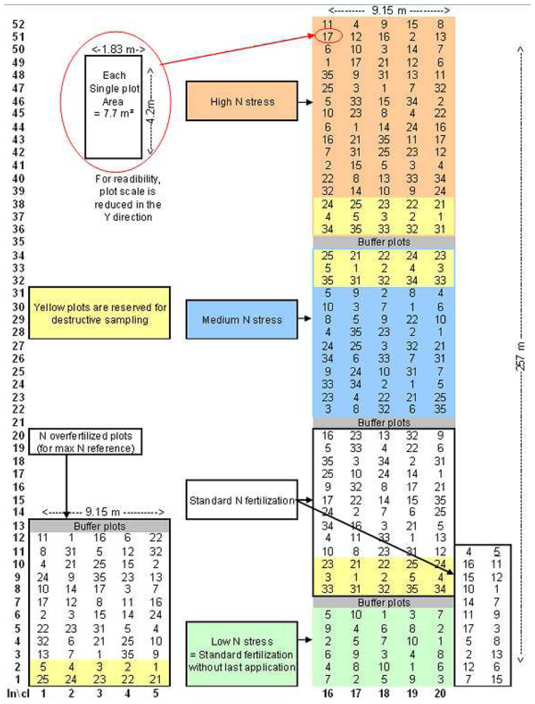
2.1 Trial plots
2.2. Ground-truth data
2.3. UAV-airborne images
- -
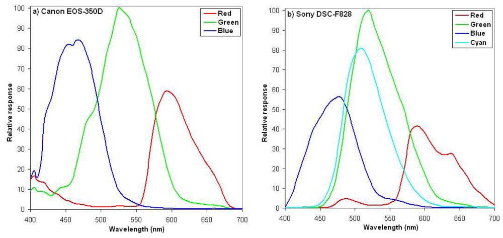
- CANON EOS 350D: a reflex camera with 8 GigaPixels classical Bayer CCD-matrix splitting the light in three channels (Red, Green, and Blue).
- -
- SONY DSC-F828: a reflex camera with 8 GigaPixels CCD-matrix splitting the light in four channels (Red, Green, Blue, and Cyan).
3. Method
3.1. Pre-processing
3.1.1. Vignetting correction
- 1)
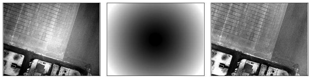
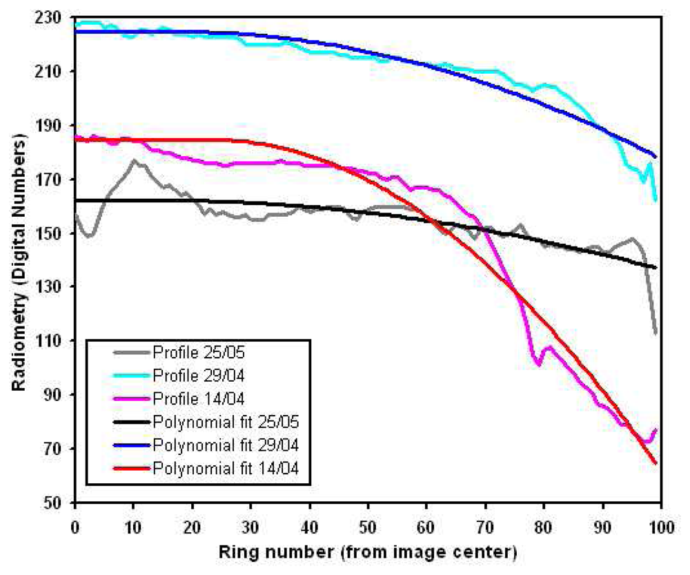
- The radial profile is derived from the mean image of all the images acquired by a single camera in the same conditions (focal distance, aperture, shutter speed), to avoid specific objects radiometric variations contribution. This mean image is split in 100, regularly spaced, concentric rings, in which the median value is calculated. The corresponding profile (the curve of the median intensity value as a function of the distance to the image centre, cf. Figure 5) is then interpolated by a two degrees polynomial function to discard the residual noise.
- 2)
- A circular image is produced, based on concentric rings. Each ring is given the value of the illumination profile polynomial fit corresponding to its distance to the centre. The number of rings depends on the size of the image to be corrected and is equal to the half of its largest dimensions to respect the Nyquist sampling theorem. A rectangle window then truncates the circular image to fit the original image dimensions, producing the vignetting image. We have chosen to lighten the corners of the image rather than darken the centre to preserve the overall image dynamics as much as possible: the area to be modified is smaller in this case. The antivignetting filter is thus the inverse of the vignetting image, produced by subtracting it to 255, minus its minimum to fix the filter minimum to zero.
- 3)
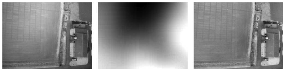
- The antivignetting filter is applied to the image to be corrected, simply summing these two images pixel to pixel. We here assume that, before summing, highest values lay near the image centre, and lowest values at the corners. Regarding the choice of corners lightning, we chose to avoid possible saturation by interpolating pixels values between the summed image minimum and the original image maximum. This interpolation also allows preserving radiometry temporal variation. Figure 6 illustrates the result obtained with this vignetting correction method.
3.1.2. Bidirectional reflectance effects correction
- 1)
- Sub-sampling of the original image. Blocks of pixels are averaged by means of a bilinear interpolation. This method has the advantage to be regular and reproducible, and rather independent of the strong dominant objects radiometry. Best results were obtained with scale factors equal to 200, thus sub-sampling for example a 2000× 2000 pixels image to a 10×10 pixels image.
- 2)
- Gaussian filtering on a 3×3 pixels window. To process all the pixels, even the first and last lines and rows of the image, we have first duplicated them, filtered the new image, and discarded them off the resulting image.
- 3)
- Over-sampling to the original size by bicubic interpolation. We have chosen to perform a bicubic interpolation because the bilinear interpolation does not translate the radiometric variations in the image with enough accuracy to provide an appropriate correction of the effects contained in the images. Minimum Curvature Splines, Thin Plate Splines, and Krigeage were also tested but resulted in too smooth results, and thus inaccurate corrections, along with a high consumption of processing time and complicated parameterization.
- 4)
- Inversion of the resulting image by subtracting it to 255, then scaling it to null origin.
- 5)
- Application of the resulting filter to the original image.
3.1.3. Geometric corrections and georeferencing
3.1.4. Intra-date and date-to-date radiometric calibration
3.2. Quantitative data extraction
3.3. Biophysical parameters estimation
- 1)
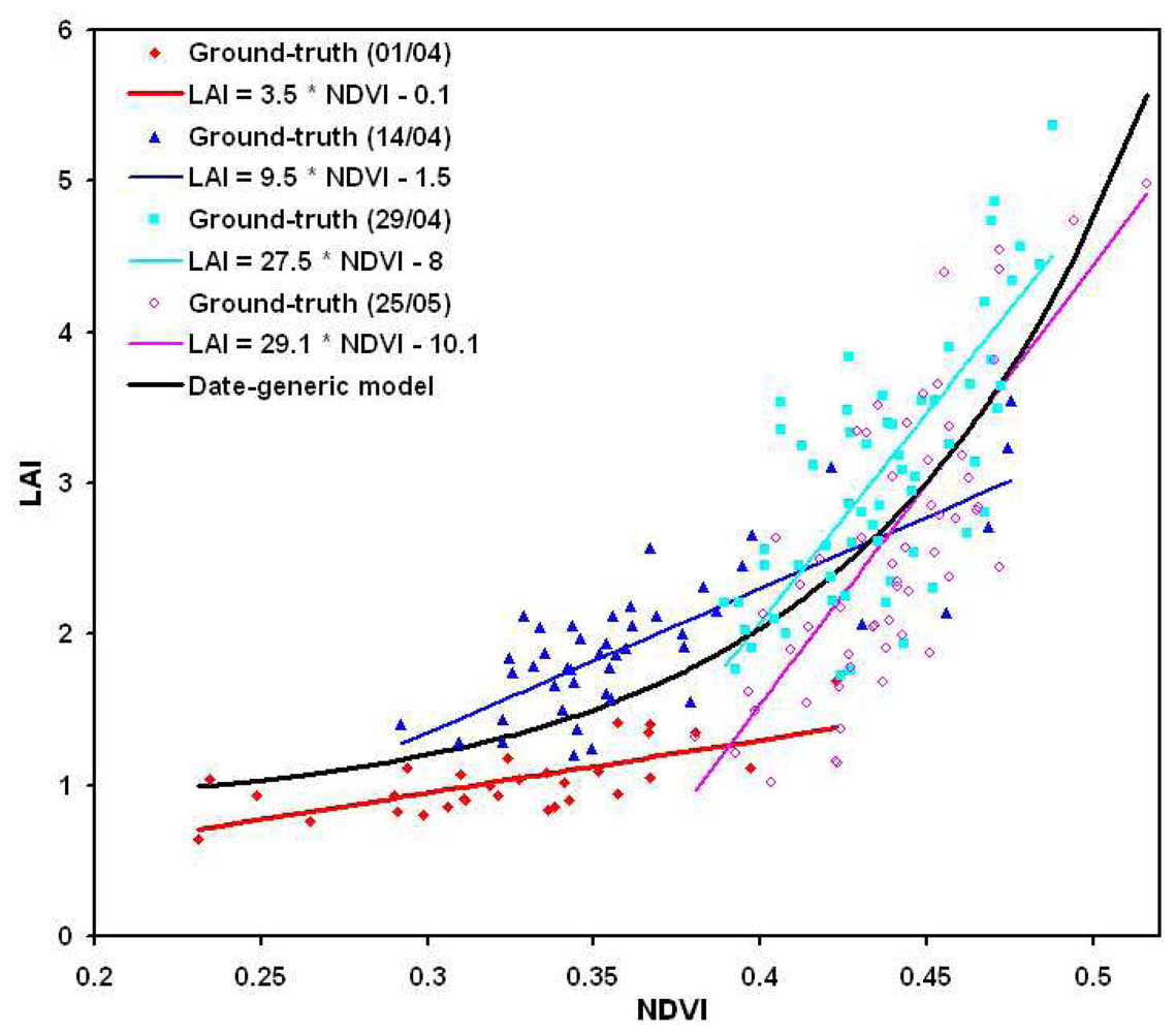
- A generic expression for any date and any genotype of wheat, taking into account the four acquisitions: 1/04, 14/04, 29/04, and 25/05, based on 192 ground-truth plots.
- 2)
- Date-specific expressions, reliable for each given date independently among 1/04, 14/04, 29/04, and 25/05, based on 30 to 50 ground-truth plots depending on the date.
4. Results and discussion
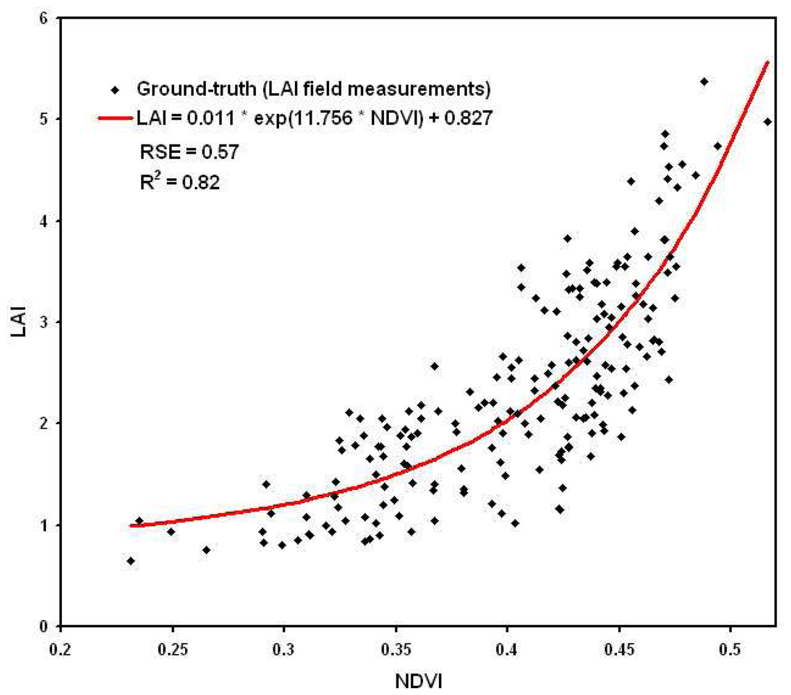
4.1. Generic relationships between LAI vs. NDVI, and QN vs. GNDVI
4.2. Date-specific relationships between LAI vs. NDVI, and QN vs. GNDVI
4.3. Cross-validation and sensibility analysis
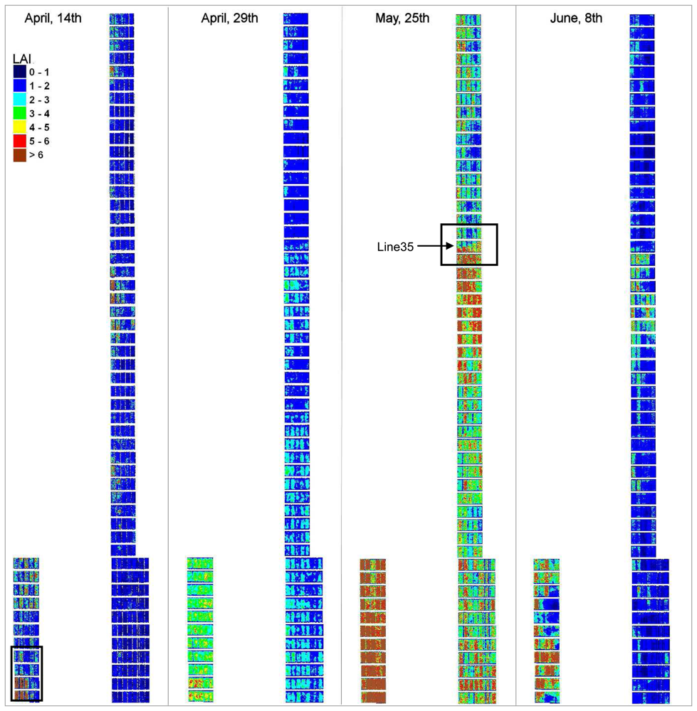
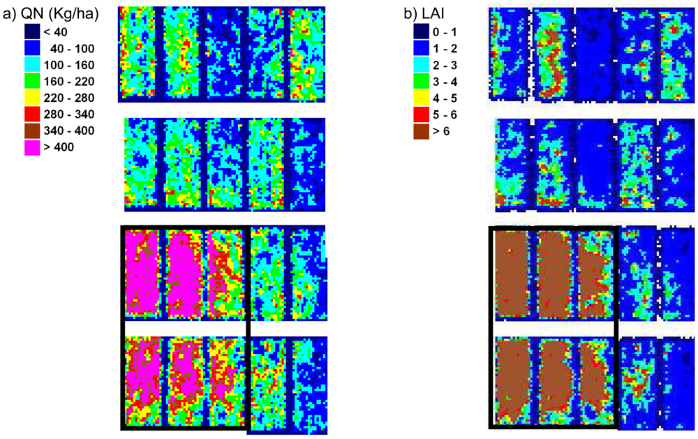
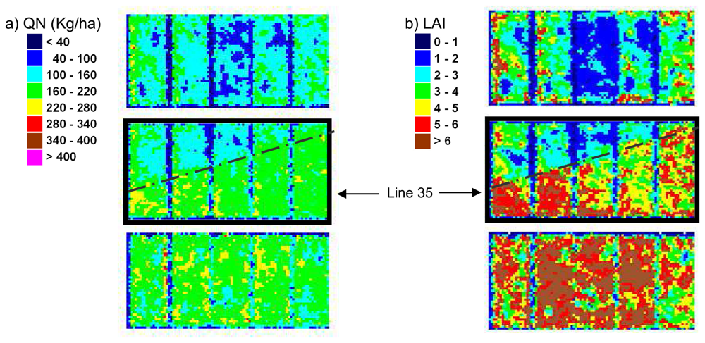
4.5. LAI and QN maps
5. Conclusion and perspectives
Acknowledgments
References
- National-Research-Council. Precision agriculture in the 21st Century: Geospatial information technologies in crop management; National Academy Press: Washington, D.C, 1997. [Google Scholar]
- Nemenyi, M.; Milics, G. Precision agriculture technology and diversity. Cereal Research Communications 2007, 35, 829–832. [Google Scholar]
- Murakami, E.; Saraiava, A.M.; Ribeiro, L.C.M.; Cugnasca, C.E.; Hirakawa, A.R.; Correa, P.L.P. An infrastructure for the development of distributed service-oriented information system for precision agriculture. Computers and Electronics in Agriculture 2007, 58, 37–48. [Google Scholar]
- Adrian, A.M.; Norwood, S.H.; Mask, P.L. Producer's perceptions and attitudes towards precision agriculture technologies. Computers and Electronics in Agriculture 2005, 48, 256–271. [Google Scholar]
- Hurley, T.M.; Oishi, K.; Malzer, G.L. Estimating the potential value of variable rate nitrogen applications: a comparison of spatial econometric and geostatistical models. Journal of Agricultural Resource Economics 2005, 30, 231–249. [Google Scholar]
- Stenberg, B.; Jonsson, A.; Borjesson, T. Use of near infrared reflectance spectroscopy to predict nitrogen uptake by winter wheat within fields with high variability in organic matter. Plant and Soil 2005, 269, 251–258. [Google Scholar]
- VanVuuren, J.A.; Meyer, J.H.; Claassens, A.S. Potential use of near infrared reflectance monitoring in precision agriculture. Communications in Soil Science and Plant Analysis 2006, 37, 3171–2184. [Google Scholar]
- Seelan, S.K.; Laguette, S.; Casady, G.M.; Seielstad, G.A. Remote sensing applications for precision agriculture: a learning community approach. Remote Sensing of Environment 2003, 88, 157–169. [Google Scholar]
- Chaerle, L.; Van Der Straeten, D. Imaging techniques and the early detection of plant stress. Trends in Plant Science 2000, 5, 295–500. [Google Scholar]
- Berri, O.; Peled, A. Spectral indices for precise agriculture monitoring. International Journal of Remote Sensing 2006, 27, 2039–2047. [Google Scholar]
- Ferwerda, J.G.; Skidmore, A.K.; Mutanga, O. Nitrogen detection with hyperspectral normalized ratio indices accross multiple plant species. International Journal of Remote Sensing 2005, 26, 4083–4095. [Google Scholar]
- Hodgen, P.J.; Raun, W.R.; Johnson, G.V.; Teal, R.K.; Freeman, K.W.; Brixey, K.B.; Martin, K.L.; Solie, J.B.; Stone, M.L. Relationship between response indices measured in-season and at harvest in winter wheat. Journal of Plant Nutrition 2005, 28, 221–235. [Google Scholar]
- Sims, D.A.; Gamon, J.A. The relationships between leaf pigment content and spectral reflectance accross a wide range of species, leaf structures and development stages. Remote Sensing of Environment 2002, 81, 337–354. [Google Scholar]
- Haboudane, D.; Miller, J.R.; tremblay, N.; Zarco-Tejada, P.J.; Dextrase, L. Integrated narrow-band vegetation indices for prediction of crop chlorophyll content for application to precision agriculture. Remote Sensing of Environment 2002, 81, 416–426. [Google Scholar]
- Thenkabail, P.S.; Smith, R.B.; de Pauw, E. Hyperspectral vegetation indices and their relationship with agricultural growth characteristics. Remote Sensing or Environment 2000, 71, 158–182. [Google Scholar]
- Franke, J.; Menz, G. Multi-temporal wheat disease detection by multi-spectral remote sensing. Precision Agriculture 2007, 8, 161–172. [Google Scholar]
- Reyniers, M.; Vrindts, E.; DeBaerdemaeker, J. Comparison of an aerial-based system and an on the ground continuous measuring device to predict yield of winter wheat. European Journal of Agronomy 2006, 34, 87–94. [Google Scholar]
- Hadria, R.; Duchemin, B.; Lahrouni, A.; Khabba, S.; Er-Raki, S.; Dedieu, G.; Chehbouni, A.G.; Olioso, A. Monitoring of irrigated wheat in a semi-arid climate using crop modeling and remote sensing data: Impact of satellite revisit time frequency. International Journal of Remote Sensing 2006, 27, 1093–1117. [Google Scholar]
- Zhao, D.G.; Li, J.L.; Qi, J.G. Identification of red and NIR spectral regions and vegetative indices for discrimination of cotton nitrogen stress and growth stage. Computers and Electronics in Agriculture 2005, 48, 155–169. [Google Scholar]
- Osborne, S.L.; Schepers, J.S.; Schlemmer, M.R. Detecting nitrogen and phosphorus stress in corn using multispectral imagery. Soil Science and Plant Analysis 2004, 35, 505–516. [Google Scholar]
- Boegh, E.; Soegaard, H.; Broge, N.; Hasager, C.B.; Jensen, N.O.; Schelde, K.; Thomsen, A. Airborne multispectral data for quantifying leaf area index, nitrogen concentration, and photosynthetic efficiency in agriculture. Remote Sensing of Environment 2002, 81, 179–193. [Google Scholar]
- Lelong, C.; Pinet, P.; Poilvé, H. Hyperspectral imaging and stress mapping in agriculture: a case study on wheat in Beauce (France). Remote Sensing of Environment 1998, 66, 179–191. [Google Scholar]
- Stone, M.L.; Solie, J.B.; Raun, W.R.; Whitney, R.W.; Taylor, S.L.; Ringer, J.D. Use of spectral radiance for correcting in-season fertilizer nitrogen deficiencies in winter wheat. Transactions of the ASAE 1996, 39, 1623–1631. [Google Scholar]
- Baret, F.; Houles, V.; Guérif, M. Quantification of plant stress using remote sensing observations and crop models: the case of nitrogen management. Journal of Experimental Botany 2007, 58, 869–880. [Google Scholar]
- Nemenyi, M.; Mesterhazi, P.A.; Pecze, Z.; Stepan, Z. The role of GIS and GPS in precision farming. Computers and Electronics in Agriculture 2003, 40, 45–55. [Google Scholar]
- Zhang, N.; Runquist, E.; Schrock, M.; Havlin, J.; Kluitenburg, G.; Redulla, C. Making GIS a versatile analytical tool for research in precision farming. Computers and Electronics in Agriculture 1999, 22, 221–231. [Google Scholar]
- Oppelt, N.; Mauser, W. Airborne visible/near infrared imaging spectrometer AVIS: design, characterization and calibration. Sensors 2007, 7, 1934–1953. [Google Scholar]
- Lamb, D.W. The use of qualitative airborne multispectral imaging for managing agricultural crops - a case study in south-eastern Australia. Australian Journal of Experimental Agriculture 2000, 40, 725–738. [Google Scholar]
- Neale, C.M.U.; Crowther, G.G. An airborne multispectral video radiometer remote-sensing system: development and calibration. Remote Sensing of Environment 1994, 49, 187–194. [Google Scholar]
- Mausel, P.W.; Everitt, J.H.; Escobar, D.E.; King, D.J. Airborne videography - Current status and future perspectives. Photogrammetric Engineering and Remote Sensing 1992, 58, 1189–1195. [Google Scholar]
- Kim, Y.; Reid, J.F. Modeling and calibration of a multispectral imaging sensor for in-field crop nitrogen assessment. Applied Engineering in Agriculture 2006, 22, 935–941. [Google Scholar]
- Beard, R.W.; McLain, T.W.; Nelson, D.B.; Kingston, D.B.; Johanson, D. Decentralized cooperative aerial-surveillance using fixed-wing miniature UAVs. Proceedings of the IEEE 2006, 94, 1306–1324. [Google Scholar]
- Majumdar, J.; Duggal, A.; Narayanan, K.G. Image exploitation - A forefront area for UAV application. Defence Science Journal 2001, 51, 239–250. [Google Scholar]
- Britton, A.; Joynson, D. An all weather millimetre wave imaging radar for UAVs. Aeronautical Journal 2001, 105, 609–612. [Google Scholar]
- Hailey, T.I. The powered parachute as a archaeological aerial reconnaissance vehicle. Archaelogical Prospection 2005, 12, 69–78. [Google Scholar]
- Casbeer, D.W.; Kingston, D.B.; Beard, R.W.; McLain, T.W. Cooperative forest fire surveillance using a team of small unmanned air vehicles. International Journal of Systems Science 2006, 37, 351–360. [Google Scholar]
- Herwitz, S.R.; Johnson, L.F.; Dunagan, S.E.; Higgins, R.G.; Sullivan, D.V.; Zheng, J.; Lobitz, B.M.; Leung, J.G.; Gallmeyer, B.A.; Aoyagi, M.; Slye, R.E.; Brass, J.A. Imaging from an unmanned aerial vehicle: agricultural surveillance and decision support. Computers and Electronics in Agriculture 2004, 44, 49–61. [Google Scholar]
- Sugiura, R.; Noguchi, N.; Ishii, K. Remote-sensing technology for vegetation monitoring using an unmanned helicopter. Biosystems Engineering 2006, 90, 369–379. [Google Scholar]
- Dean, C.; Warner, T.A.; McGraw, J.B. Suitability of the DCS460c colour digital camera for quantitative remote sensing analysis of vegetation. ISPRS Journal of Photogrammetry and Remote Sensing 2000, 55, 105–118. [Google Scholar]
- Shortis, M.R.; Seager, J.W.; Harvey, E.S.; Robson, S. The influence of Bayer filters on the quality of photogrammetric measurements; Videometrics VIII: San Jose, Canada, 2005; Beraldin, J.-A., El-Hakim, S.F., Gruen, A., Walton, J.S., Eds.; pp. 164–171. [Google Scholar]
- Smith, W.J. Modern Optical Engineering; Hill, M., Ed.; SPIE Press: New York, 2000; p. 617 pages. [Google Scholar]
- Gitin, A.V. Integral description of physical vignetting. Soviet Journal of Optical Technology 1993, 60, 556–558. [Google Scholar]
- Leong, F.J.; Brady, M.; McGee, J. Correction of uneven illumination (vignetting) in digital microscopy images. Journal of Clinical Pathology 2003, 56, 619–621. [Google Scholar]
- Lumb, D.H.; Finoguenov, A.; Saxton, R.; Aschenbach, B.; Gondoin, P.; Kirsch, M.; Stewart, I.M. In-orbit vignetting calibrations of XMM-Newton telescopes. Experimental Astronomy 2003, 15, 89–111. [Google Scholar]
- Mansouri, A.; Marzani, F.S.; Gouton, P. Development of a protocol for CCD calibration: application to a multispectral imaging system. International Journal of Robotics and Automation 2005, 20, 94–100. [Google Scholar]
- Sim, D.G. New panoramic image generation based on modeling of vignetting and illumination effects. Advances in multimedia information processing - PT1: Lecture notes in computer sciences 2005, 3767, 1–12. [Google Scholar]
- Yu, W. Practical anti-vignetting methods for digital cameras. IEEE Transactions on Consumer Electronics 2004, 50, 975–983. [Google Scholar]
- Klimentev, S.I. Vignetting in telescope systems with holographic image correction. Journal of Optical Technology 2002, 69, 385–391. [Google Scholar]
- Powel, I. Technique employed in the development of antivignetting filters. Optical Engineering 1997, 36, 268–272. [Google Scholar]
- Dean, C.; Warner, T.A.; McGraw, J.B. Suitability of the DCS460c colour digital camera for quantitative remote sensing analysis of vegetation. ISPRS Journal of Photogrammetry and Remote Sensing 2000, 55, 105–118. [Google Scholar]
- Edirisinghe, A.; Chapman, G.E.; Louis, J.P. Radiometric corrections for multispectral airborne video imagery. Photogrammetric Engineering and Remote Sensing 2001, 67, 915–922. [Google Scholar]
- Sawchuk, A.A. Real-time correction of intensity nonlinearities in imaging systems. IEEE Transactions on Computers 1977, 26, 34–39. [Google Scholar]
- Asada, N.; Amano, A.; Baba, M. Photometric calibration of zoom lens systems. 13th International Pattern Recognition Conference, Vienne, Austria; Recognition, T. I. A. f. P., Ed.; 1996; pp. 186–190. [Google Scholar]
- Causi, G.L.; Luca, M.D. Optimal subtraction of OH airglow emission: A tool for infrared fiber spectroscopy. New Astronomy 2005, 11, 81–89. [Google Scholar]
- Hapke, B. Bidirectional reflectance spectroscopy. 1. Theory. Journal of Geophysical Research 1981, 86, 3039–3054. [Google Scholar]
- Pinty, B.; Ramon, D. A simple bidirectional reflectance model for terrestrial surfaces. Journal of Geophysical Research 1986, 91, 7803–7808. [Google Scholar]
- Roujean, J.L.; Leroy, M.; Deschamps, P.Y. A bidirectional reflectance model of the Earth's surface for the correction of remote-sensing data. Journal of Geophysical Research 1992, 97, 20455–20468. [Google Scholar]
- Fahnestock, J.D.; Schonwengerdt, R.A. Spatially-variant contrast enhancement using local range modification. Optical Engineering 1983, 22, 378–381. [Google Scholar]
- Nobrega, R.A. Comparative analysis of atomatic digital image balancing and standard histogram enhancement techniques in remote sensing imagery. Revista Brazileira de Cartographia 2002, 56/01. [Google Scholar]
- Zitova, B.; Flusser, J. Image registration methods: a survey. Image and vision Computing 2003, 21, 977–1000. [Google Scholar]
- Goshtasby, A. Registration of images with geometric distorsions. IEEE Transactions on Geosciences and Remote Sensing 1988, 26, 60–64. [Google Scholar]
- Richards, J.A. Error Correction and Registration of Image Data. In Remote Sensing Digital Image Analysis; Chapter 1; Springer-Verlag (eds): Berlin, 1999; pp. 56–59. [Google Scholar]
- Tucker, C.J. Red and photographic infrared linear combinations for monitoring vegetation. Remote Sensing of Environment 1979, 8, 127–150. [Google Scholar]
- Cihlar, J.; St-Laurent, L.; Dyer, J. Relation between the normalized vegetation index and ecological variables. Remote Sensing of Environment 1991, 35, 279–298. [Google Scholar]
- Rondeaux, G.; Steven, M.; Baret, F. Optimization of soil-adjusted vegetation indices. Remote Sensing of Environment 1996, 55, 95–107. [Google Scholar]
- Gitelson, A.A.; Kaufman, Y.J.; Merzlyak, M.N. Use of green channel in remote sensing of global vegetation from EOS-MODIS. Remote Sensing of Environment 1996, 58, 289–298. [Google Scholar]
- Huete, A.R. A soil-adjusted vegetation index (SAVI). Remote Sensing of Environment 1988, 25, 295–309. [Google Scholar]
- Houlès, V.; Guérif, M.; Mary, B. Elaboration of a nitrogen nutrition indicator for winter wheat based on leaf area index and chlorophyll content for making nitrogen recommendations. European Journal of Agronomy 2007, 27, 1–11. [Google Scholar]
- Wenjiang, H.; Jihua, W.; Zhijie, W.; Jiang, Z.; Liangyun, L.; Jindi, W. Inversion of foliar biochemical parameters at various physiological stages and grain quality indicators of winter wheat with canopy reflectance. International Journal of Remote Sensing 2004, 25, 2409–2419. [Google Scholar]
- Das, D.K.; Mishra, K.K.; Kalra, N. Assessing growth and yield of wheat using remotely-sensed canopy temperature and spectral indices. International Journal of Remote Sensing 1993, 14, 3081–3092. [Google Scholar]
- Moulin, S.; Milla, R.Z.; Guérif, M.; Baret, F. Characterizing the spatial and temporal variability of biophysical variables of a wheat crop using hyper-spectral measurements. IEEE International Geoscience and Remote Sensing Symposium (IGARSS), Toulouse, France; IEEE (Eds), Ed.; 2003; pp. 2206–2208. [Google Scholar]


| Channel | Canon EOS-350D | Sony DSC-F828 | Landsat, Quickbird, Ikonos | SPOT |
|---|---|---|---|---|
| R | 570-640 nm | 570-650 nm | 630-690 nm | 610-680 nm |
| G | 490-580 nm | 490-570 nm | 520-600 nm | 500-590 nm |
| B | 420-500 nm | 430-510 nm | 450-520 nm | - |
| NIR | 720-850 nm | 720-850 nm | 760-900 nm | 790-890 nm |
| Name of Indices tested in this study | Index expression | Reference |
|---|---|---|
| NDVI (normalized difference vegetation index) | (NIR – R)/(NIR + R) | [63] |
| SAVI (soil-adjusted vegetation index) | (1 - L)(NIR – R)/(NIR + R - L) with L=0.5 | [67] |
| GNDVI (green normalized difference vegetation index) | (NIR – G)/(NIR + G) | [20] |
| GI (greenness index) | (R – V)/(R + V) | [66] |
| Derived parameter | RSE | Mean relative error | Min. relative error | Correlation coefficient |
|---|---|---|---|---|
| LAI | 0.6 m2/m2 | 17% | 8% | 0.82 |
| QN | 19 Kg/ha | 13% | 6% | 0.92 |
| Parameter | Date | A | B | RSE | MRE |
|---|---|---|---|---|---|
| LAI | 01/04 | 3.5 | -0.1 | 0.2 m2/m2 | 19% |
| 14/04 | 9.5 | -1.5 | 0.3 m2/m2 | 15% | |
| 29/04 | 27.7 | -8.0 | 0.5 m2/m2 | 16% | |
| 25/25 | 29.1 | -10.1 | 0.6 m2/m2 | 23% | |
| QN | 01/04 | 197 | -44 | 4 Kg/ha | 16% |
| 14/04 | 700 | -220 | 11 Kg/ha | 18% | |
| 29/04 | 1580 | -627 | 17 Kg/ha | 17% | |
| 25/25 | 1234 | -457 | 23 Kg/ha | 18% |
| LAI vs NDVI | A | B | C | RSE | MLAI | DLAI | CC Valid. |
|---|---|---|---|---|---|---|---|
| Initial | 0.011 | 11.76 | 0.83 | 0.57 | 2.34 | 0 | 0.83 |
| Test 1 | 0.019 | 10.69 | 0.70 | 0.56 | 2.34 | 0.02 | 0.81 |
| Test 2 | 0.012 | 11.42 | 0.78 | 0.53 | 2.33 | 0.14 | 0.81 |
| Test 3 | 0.014 | 11.32 | 0.73 | 0.57 | 2.32 | 0.02 | 0.79 |
| Test 4 | 0.019 | 10.65 | 0.72 | 0.56 | 2.34 | 0.02 | 0.78 |
| Test 5 | 0.016 | 10.99 | 0.76 | 0.58 | 2.34 | 0.01 | 0.82 |
| Test 6 | 0.008 | 12.34 | 0.93 | 0.57 | 2.36 | 0.02 | 0.86 |
| Test 7 | 0.01 | 11.97 | 0.85 | 0.59 | 2.35 | 0.06 | 0.85 |
| Test 8 | 0.014 | 11.22 | 0.73 | 0.57 | 2.33 | 0.01 | 0.8 |
| Test 9 | 0.012 | 11.61 | 0.86 | 0.57 | 2.32 | 0.08 | 0.81 |
| Test 10 | 0.016 | 11.03 | 0.80 | 0.57 | 2.34 | 0.06 | 0.83 |
| QN vs GDVI | A | B | C | RSE | MQN | DQN | CC Valid. |
|---|---|---|---|---|---|---|---|
| Initial | 17.8 | 5.2 | -82.4 | 19 | 89 | 0 | 0.93 |
| Test 1 | 20.8 | 4.9 | -88.1 | 20.5 | 90 | 1.93 | 0.93 |
| Test 2 | 11.7 | 5.9 | -68.1 | 19.3 | 87 | 3.66 | 0.92 |
| Test 3 | 13.3 | 5.6 | -70.4 | 20.4 | 92 | 4 | 0.92 |
| Test 4 | 18.6 | 5.1 | -86.3 | 20.3 | 91 | 6.7 | 0.92 |
| Test 5 | 23.2 | 4.7 | -96.7 | 19.6 | 91 | 4.07 | 0.89 |
| Test 6 | 20.7 | 4.9 | -89.8 | 19.9 | 88 | 1.07 | 0.9 |
| Test 7 | 18.5 | 5 | -82.2 | 19.9 | 91 | 9.84 | 0.91 |
| Test 8 | 22.7 | 4.7 | -93.9 | 18.7 | 87 | 4.44 | 0.9 |
| Test 9 | 19.6 | 5 | -85.7 | 19.8 | 90 | 4.49 | 0.92 |
| Test 10 | 17.7 | 5.1 | -80.4 | 19.6 | 88 | 4.4 | 0.92 |
| Plot | Cultivar | Measured LAI (06/04) | Interpolated LAI (14/04) | Calculated mean LAI (14/04) | Measured QN (06/04) | Interpolated QN (14/04) | Calculated mean QN (14/04) |
|---|---|---|---|---|---|---|---|
| 0101 | 25 | 1.7 | 2.7 | 3.5 | 55 | 143 | 251 |
| 0404 | 25 | 1.1 | 1.6 | 1.8 | 36 | 61 | 59 |
| 0102 | 24 | 1.2 | 2.1 | 3.1 | 44 | 76 | 219 |
| 0605 | 24 | 0.8 | 1.2 | 1.5 | 27 | 58 | 81 |
| 0103 | 23 | 1.2 | 2.1 | 2.5 | 36 | 72 | 91 |
| 0502 | 23 | 1.2 | 1.9 | 1.8 | 39 | 76 | 88 |
| 0201 | 5 | 2.4 | 3.5 | 3.8 | 78 | 118 | 124 |
| 0504 | 5 | 1.4 | 2.5 | 2.0 | 44 | 168 | 156 |
| 0202 | 4 | 2.3 | 3.2 | 3.7 | 78 | 123 | 150 |
| 0505 | 4 | 1.1 | 1.9 | 1.5 | 38 | 152 | 160 |
| 0203 | 3 | 1.9 | 3.1 | 2.8 | 55 | 184 | 166 |
| 0602 | 3 | 1.4 | 2.3 | 1.8 | 43 | 149 | 148 |
© 2008 by the authors; licensee Molecular Diversity Preservation International, Basel, Switzerland. This article is an open-access article distributed under the terms and conditions of the Creative Commons Attribution license ( http://creativecommons.org/licenses/by/3.0/).
Share and Cite
Lelong, C.C.D.; Burger, P.; Jubelin, G.; Roux, B.; Labbé, S.; Baret, F. Assessment of Unmanned Aerial Vehicles Imagery for Quantitative Monitoring of Wheat Crop in Small Plots. Sensors 2008, 8, 3557-3585. https://doi.org/10.3390/s8053557
Lelong CCD, Burger P, Jubelin G, Roux B, Labbé S, Baret F. Assessment of Unmanned Aerial Vehicles Imagery for Quantitative Monitoring of Wheat Crop in Small Plots. Sensors. 2008; 8(5):3557-3585. https://doi.org/10.3390/s8053557
Chicago/Turabian StyleLelong, Camille C. D., Philippe Burger, Guillaume Jubelin, Bruno Roux, Sylvain Labbé, and Frédéric Baret. 2008. "Assessment of Unmanned Aerial Vehicles Imagery for Quantitative Monitoring of Wheat Crop in Small Plots" Sensors 8, no. 5: 3557-3585. https://doi.org/10.3390/s8053557