Working Principle Simulations of a Dynamic ResonantWall Shear Stress Sensor Concept

Mechanical Department, University of Wyoming, USA; Laboratory for Shock Wave and Detonation
*
Author to whom correspondence should be addressed.
Sensors 2008, 8(4), 2707-2721; https://doi.org/10.3390/s8042707
Submission received: 26 November 2007
/
Accepted: 1 April 2008
/
Published: 17 April 2008
Abstract
:This paper discusses a novel dynamic resonant wall shear stress sensor concept based on an oscillating sensor operating near resonance. The interaction between the oscillating sensor surface and the fluid above it is modelled using the unsteady laminar boundary layer equations. The numerical experiment shows that the effect of the oscillating shear stress is well correlated by the Hummer number, the ratio of the steady shear force caused by the outside flow to the oscillating viscous force created by the sensor motion. The oscillating shear stress predicted by the fluid model is used in a mechanical model of the sensor to predict the sensor's dynamic motion. Static calibration curves for amplitude and frequency influences are predicted. These results agree with experimental results on some extent, and shows some expectation for further development of the dynamic resonant sensor concept.
1. Nomenclature
| m | Sensor Mass |
| xs | Sensor Position |
| b | Damping Coefficient |
| k | Spring Constant |
| Fm | Time-Dependent Excitation Force |
| Ff | Time-Dependent Shear Force |
| Ls | Characteristic Length of Sensor |
| Ly | Vertical Penetration Depth of Oscillating Sensor |
| f | Sensor Frequency |
| xs | Sensor Position |
| b | Damping Coefficient |
| k | Spring Constant |
| Fm | Time-Dependent Excitation Force |
| Ff | Time-Dependent Shear Force |
| Ls | Characteristic Length of Sensor |
| Ly | Vertical Penetration Depth of Oscillating Sensor |
| f | Sensor Frequency |
| a | Sensor Amplitude |
| U | Characteristic Flow Velocity Scale |
| L | Characteristic Flow Length Scale |
| τ0 | Mean Wall Shear Stress |
| ρ | Density of Flow |
| a* | Amplitude Ratio |
| Y* | Penetration Depth Ratio |
| L* | Flow/Sensor Length Ratio |
| ν | Kinematic Viscosity |
| Re | Reynolds Number |
| St | Strouhal Number |
| Hr | Hummer Number |
| x,y | Cartesian Coordinates |
| u,v | x and y Velocity Components |
| u′, v′ | x and y Fluctuating Velocity |
| x*, y* | Normalized Cartesian Coordinates |
| u*,v* | x and y Normalized Fluctuating Velocity Components |
| u*′, v*′ | x and y Normalized Fluctuating Velocity Components |
| t | Time |
| μ | Dynamic Viscosity |
| Ue | Edge Velocity |
| X | Non-Dimensional Streamwise Coordinate |
| T | Non-Dimensional Time |
| η | Non-Dimensional Vertical Coordinate |
| P1,P2,P3 | Known values in the simplified boundary layer equations |
| U0 | Edge Velocity at t=0 |
| ψ | Stream Function |
| Us | Sensor Velocity |
| P, Q, R | Locations Where Differences are Determined in Zig-Zag Scheme |
| < > | Time Average |
| ω | Angular Frequency |
| Fluctuating Skin Friction | |
| τ | Wall Shear Stress |
| A | Peak-to-peak Amplitude of the Sensor |
| Aτ = 0 | Peak-to-peak Amplitude of the Sensor at zero shear stress level |
1.1. Subscripts
| pp | Peak-to-Peak |
| s | Sensor |
| rms | Root-Mean Square Value |
| Blasius | Blasius Boundary Layer Result |
2. Introduction
The development of surface shear stress sensor has been studied extensively. The need for wall shear stress measurements is important in both fundamental fluid mechanics problems and real-world systems. Some kind of sensors that have been investigated for years at large scales are being reduced in size to investigate benefits arising from scaling. Direct force balances, thermal sensors, and sensors measuring points in the velocity profile have all been investigated recently at small-scale. At the large scale, these sensors suffer from several shortcomings. As a result, measurement techniques such as oil-film interferometry are gaining widespread use for mean surface shear stress measurements. Due to the nature of the oil-film technique, it is likely that its use will be limited outside the laboratory environment, and it is not a candidate for fluctuating measurements. More details about surface shear stress measurement methods can be found in related literatures written by Winter, [1] Haritonidis, [2] and Naughton and Sheplak [3].
Benefits of creating sensors at the small scale are possible because of the advances in microelectrical-mechanical system (MEMS) and micromachining technologies now available. The approach to date has primarily been to reduce the size of conventional sensors, and it has met with mixed success. A brief description of experience with miniature force-balance techniques is provided below. Other approaches (velocity-based sensors, thermal, and surface acoustic wave sensors) can be found in the literature (see Naughton and Sheplak [3] for an overview).
Small-scale implementations of direct force balance methods have been around for 15 years since Schmidt et al. implemented the first prototype sensor [4]. Subsequent modifications have improved on this original design. In all these designs, elastic legs (tethers) support a floating element. As shear stress is applied to the sensor surface, the sensor deflects laterally. Capacitive, [4, 5] piezo-resistive, [6–8] and photo-electric [9, 10] methods have been used to determine the position of the sensor. In another design, Pan et al. [11] developed a sensor that incorporated an electro-static comb-finger design that could be used for capacitive sensing of floating element position or could be used to actuate the sensor. More recently, Zhe et al. [12] has a preliminary design for a cantilever beam sensor that also uses capacitive sensing to measure displacement. Horowitz et al. [13] have recently demonstrated the use of Moire interferometry as a means of sensing the displacement of a floating element. Of these sensor concepts, only those of Padmanabhan et al. [9] and Horowitz et al. [13] have been dynamically calibrated (to 4 kHz). A drawback of floating element designs is their limitations in dirty environments due to the necessary gaps between the floating element and the surrounding surface. The sensor of Padmanabhan et al. [9] required a remote light source that made the sensor sensitive to vibration. In summary, balance techniques appear to show promise, but a fully characterized prototype with the necessary features for fluctuating surface shear stress measurements has not yet been developed.
This paper numerically describes characteristics of a novel wall shear stress sensing concept that was developed by Professors at UW ActiveAero Center. The novel sensor studied here is a dynamic resonant sensor that takes advantage of the sensitivity of a resonant system to small changes in its environment. The challenge here is to design the resonant system such that it is highly sensitive to small wall shear stress forces and insensitive to large pressure forces. In addition, the system should only be weakly sensitive to other changes in the system.
To develop this sensor, both experimental work and modelling of the sensor concept have been undertaken. A prototype sensor has been fabricated and tested and shows sensitivity to wall shear stress as expected. The present sensor is sensitive to wall shear stress due to the complex interaction between the oscillating sensor and the fluid above it. The results of this work are reported by Armstrong [14]. To complement the experimental effort, the development of a coupled fluid/mechanical model of the sensor has been undertaken to understand the operating principles of the sensor. The results from the model provide a solid basis for understanding the sensor, and, with further validation, the model will provide a tool for optimizing the sensor concept.
3. Dynamic Resonant Shear Stress Sensor Concept
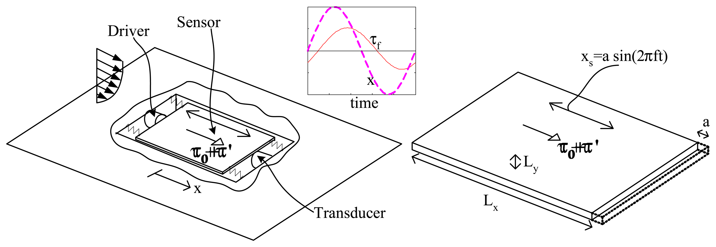
The idea of using a dynamic resonant device arose from the sensitivity of resonant devices to small changes in their environment. Figure 1 shows a schematic of the sensor with its important components and parameters. The sensor is forced to oscillate near resonance using a driving device, and a position transducer measures the location of the sensor. The sensor can be modelled as a forced second-order system with an additional forcing term supplied by the unsteady shear force that develops on the sensor surface exposed to the flow:
The unsteady shear force Ff is dependent on the interaction between the oscillating sensor and the boundary layer flow above the sensor. As will be shown, the fluid response time is finite, and thus the shear force lags the sensor motion. This phase lag ensures that the shear force is not proportional to position or velocity, and thus introduces amplitude difference due to this phase lag.
The prototype design of this sensor is shown in figure 2 where both an image of the sensor surface (a) and a solid model of the sensor (b) are shown. The sensor is made from a single piece of stainless steel, and material is removed using electrical discharge machining (EDM). The active sensor surface is connected to the main body through thin sensor legs (tethers) that provide high compliance thus providing resonance over a small range of frequency (i.e. it is a high Q system). The sensor is driven by the interaction between the driving magnet and a hand-wound magnetic solenoid that is driven by the amplified output of a signal generator. The signal generator is used to control the amplitude and frequency of the driving signal. A magnetic Hall probe is used to measure the sensor position whose output is linearly related to position. The decrease of the magnetic field with the square of the distance from the solenoid ensures very little effect of the solenoid on the Hall probe output. The active sensing area of the prototype sensor is approximately 10 mm square. This sensor may be operated in an open loop or closed loop configuration. To determine the quantities important to the fluid/structure interaction associated with this sensor, non-dimensional analysis of the equations governing the fluid flow have been carried out. Some useful parameters given in figure 1 yield several dimensional groups summarized in table 1. The amplitude ratio represents the amount that the sensor moves compared to the length of the sensor. The penetration depth ratio represents the distance that the sensor affects the flow in the vertical direction (Ly) to the sensor length (Ls). Here, viscous scaling for the vertical length scale similar to that used for a Stokes layer is used
. The sensor-to-flow length scale ratio represents the ratio of the characteristic length of the sensor to the length scale associated with the flow field. As will be demonstrated by the non-dimensionalization of the boundary layer equations, the most important non-dimensional quantity is the Hummer number, the ratio of the forces due to the mean flow to the unsteady forces created by the sensor motion.
The boundary layer equations (momentum and mass) are decomposed into a mean and a fluctuating equations. The fluctuating equations are then non-dimensionalized using the following scaling:
Substituting this scaling into the fluctuating boundary layer equation yields
Equation 2 has two different terms that arise from the original convective terms: terms that represent the convection of velocity fluctuations by the mean flow and other terms that represent convection of velocity fluctuations by the fluctuating flow. In order to be sensitive to shear stress for this sensor, these terms must both survive and must be of order one:
The first parameter in equation 3 represents the relative motion of the sensor indicating that the sensor has to have an appreciable movement relative to its length. To interpret the second parameter in equation 3, assume the vertical penetration depth length scale Ly scales as in Stokes flow [15]
which yields the following dimensionless parameter:
This dimensionless group represents the ratio of the shear stress force on the sensor due to the mean flow above the sensor to the viscous force on the sensor due to its oscillating movement. Due to its importance to the current sensor, this parameter has been named the “Hummer Number.” The significance of the Hummer number having to be of order one indicates that the oscillation has to be such that it creates unsteady forces on the sensor that are of the order of the mean shear force exerted on the sensor. This requirement provides one guide for designing sensors operating under different conditions.
4. Model Description
4.1. Fluid Model
There are several numerical methods for solving the unsteady boundary layer equations in differential form. Finite difference methods that have been used for these flows include the Crank-Nicolson scheme [16], the characteristic scheme [17, 18], and the Keller's Box method [19]. Cebeci provides a detailed introduction of solution methods for boundary layer flows [19]. In this study, a modified box scheme is employed that uses a zig-zag scheme to calculate regions of reverse flow [19].
4.1.1. Boundary Layer Flow Simulations
Non-Dimensional Control Equations The two-dimensional unsteady boundary-layer equations are given by
In terms of the dependent dimensionless variables defined by
and an independent dimensionless variable
the boundary layer equations (equations 6 and 7) become
where
Equation 8 is a third-order non-linear ordinary differential equation. This equation are solved using a linearized method.
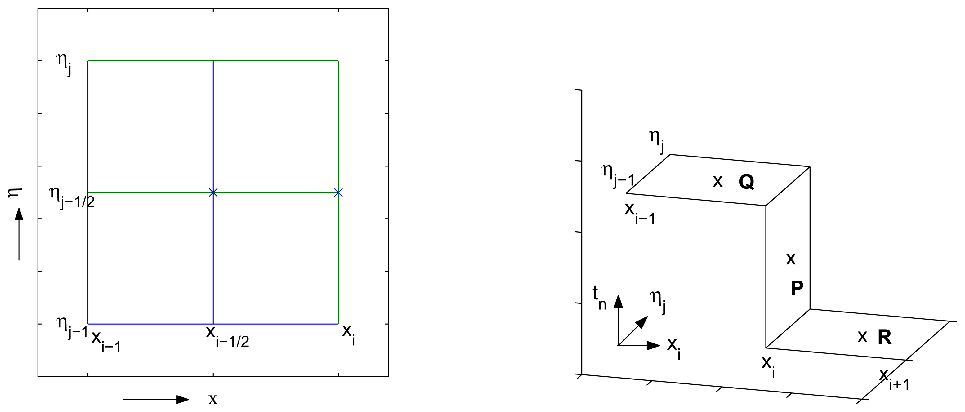
Solution Methods To solve equation 8 with corresponding initial and boundary conditions, Keller's Box method, which is a two point finite difference scheme, is used. As shown in Fig. 3, the difference approximation for equation 8 is taken at xi,
and
,
.
A zig-zag difference scheme is used to calculate regions that contain reverse flow According to the local characteristic velocity, the appropriate finite difference scheme for equation 8 is selected. If
, the standard Box method is used. If
, zig-zag scheme is used in order to include information from upstream. For zig-zag scheme quantities are centered at point P(see fig. 3), and uses quantities centered at P, Q and R, where
The resulting system of equations from Box and zig-zag schemes is both implicit and nonlinear. The system of equations is solved using a block-elimination method.
Boundary Conditions Equation 8 is parabolic, and thus boundary conditions are required at the inlet, on the surface, and in the free stream. The boundary conditions on the surface enforce the no-slip condition. A time-dependent velocity is prescribed for those grid points that represent the sensor surface because a moving dynamic sensor is being modelled, and zero velocity is prescribed elsewhere on the surface. The time-dependent wall velocity of the sensor grid points is given by
where Us,max = 2πfa/Ue. Whereas the upper boundary condition is simply a prescribed edge velocity Note that pressure gradients can be imposed by varying this free-stream velocity along the surface. The inflow boundary condition is prescribed as a laminar boundary layer by solving
Initial Conditions Initial conditions must be provided to solve equation 8. The initial conditions are determined by solving 8 without time term. The initial conditions represent a laminar boundary layer subject to a pressure gradient for a fixed wall. Thus, the solution of the time dependent problem will capture the transient behavior of the sensor during startup, and the simulation must be run for a sufficient amount of time to achieve an asymptotic result.
4.2. Mechanical Dynamic Resonant Device Model
The mechanical model is constructed by the application of Newton's second law in the presence of driving, elastic-structural, inertial and fluid forces. Equation 1 is used to describe the mechanical model. Fourth-order Runge-Kutta integration is used to solve this equation to determine the sensor position as a function of time.
4.3. Assumptions Inherent to the Models
In the flow model, the gap effects between dynamic sensor and the non-moving surface have been neglected. There is expected to be some damping effect from this region, but it has been neglected to simplify the calculations. In the mechanical model, damping ratio changes due to the influence of the non-linear spring stiffness (static equilibrium position changes) for different mean shear force acting on the dynamic sensor have been neglected.
5. Results
5.1. Fluid Model Results
The fluid model discussed above has been used to simulate the sensor behavior in a laminar boundary layer flow. The sensor is located halfway down a flat plate and has a length 1/10th of plate length, which yields a constant flow/sensor length scale ratio L* of 0.1. All other parameters (Re, Hr, St, a*) are varied in the simulations.
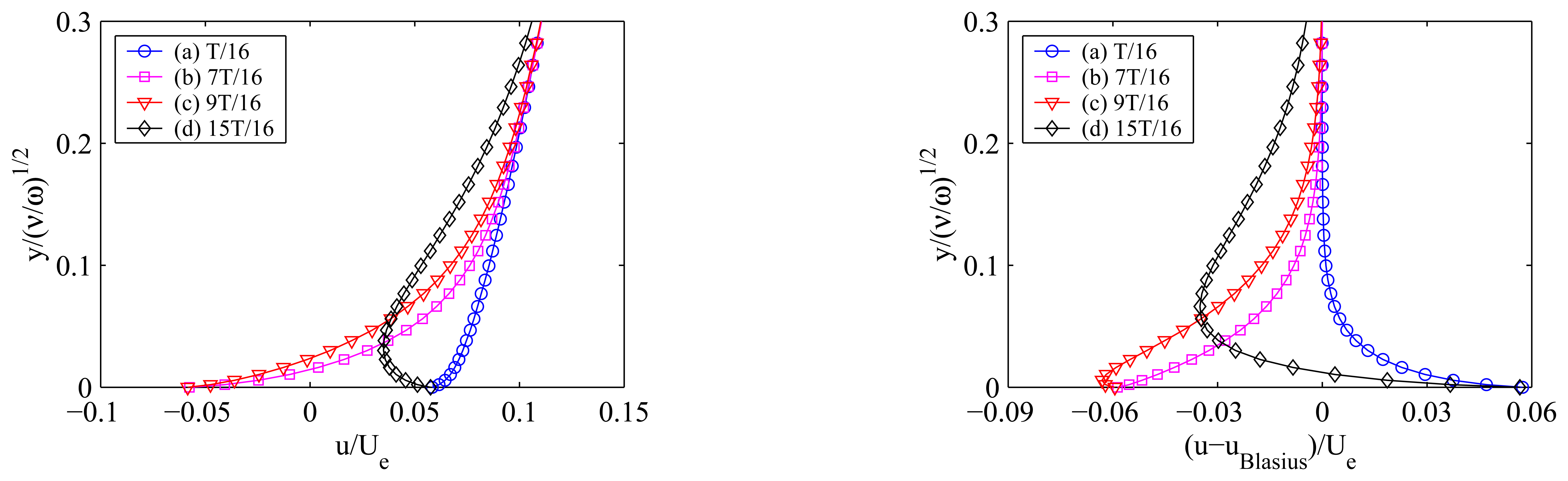
The non-linear interaction between the sensor and fluid is key to the success of this sensor. This is evident in figure 4 where the velocity profiles are shown at four different times during an oscillation cycle. Left side in figure 4 shows the non-dimensional velocity near the wall and right side of figure 4 shows the velocity in the same location with the Blasius velocity subtracted. Due to the no-slip condition on the sensor surface, the velocity directly above the surface matches that of the sensor. At distances further above the wall, it takes time for momentum to diffuse upward and thus the velocity at these points lags the sensor velocity. This is evident in the velocity profile at point d (15 T/16) where the sensor is moving forward and the velocity above the wall is lagging behind. The details of the velocity profile near the wall have an obvious impact on the fluctuating shear stress force experienced by the sensor. Another important result is that the region above the wall that the sensor's motion affects is relatively small for the conditions shown here. In figure 4, it is evident that the fluctuating velocity near the wall looks much like a Stokes layer. The penetration distance of the fluctuating velocity is smaller than that of a typical Stokes layer, which probably results from convection of the momentum imparted by the wall by the mean velocity above the wall.
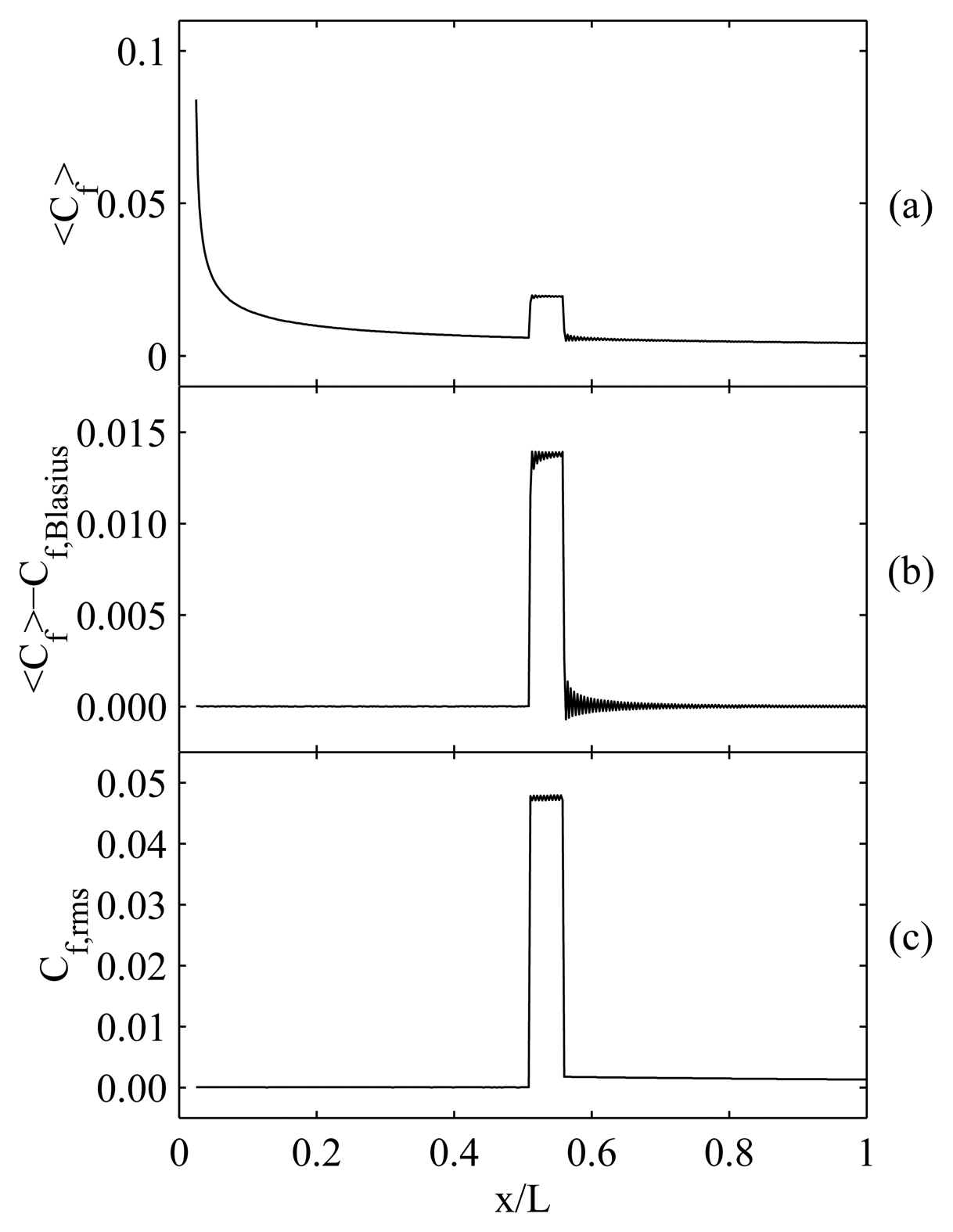
Changes in the shear stress distribution near the sensor are expected from the time dependent velocity profiles imposed by the oscillating sensor. The mean and fluctuating shear stress in the boundary of the sensor are shown in figure 5. In Figure 5(a), it is interesting that the oscillating shear stress causes a local elevation in the mean skin friction. Figure 5(b) shows the mean shear with the Blasius result removed revealing that the increase in shear stress is isolated to the region directly adjacent to the sensor. There are some oscillations seen in Figure 5(b) from numerical artifacts. The rms skin friction is shown in Figure 5(c) where it can be seen that the fluctuating shear stress caused by the sensor is actually several times the mean shear at the sensor location.
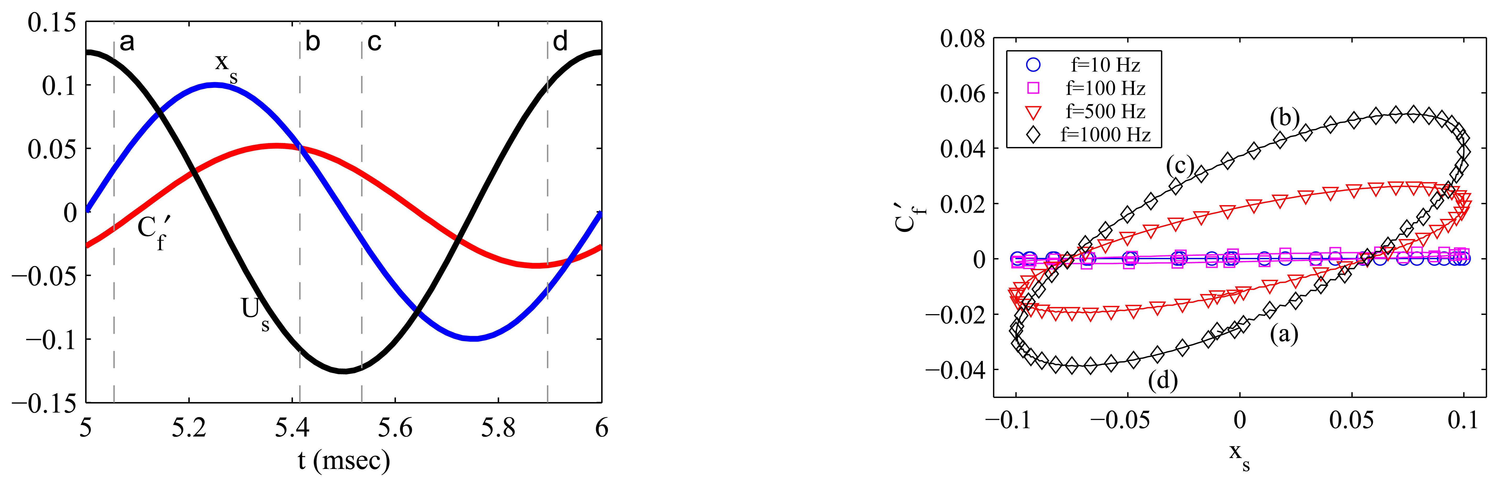
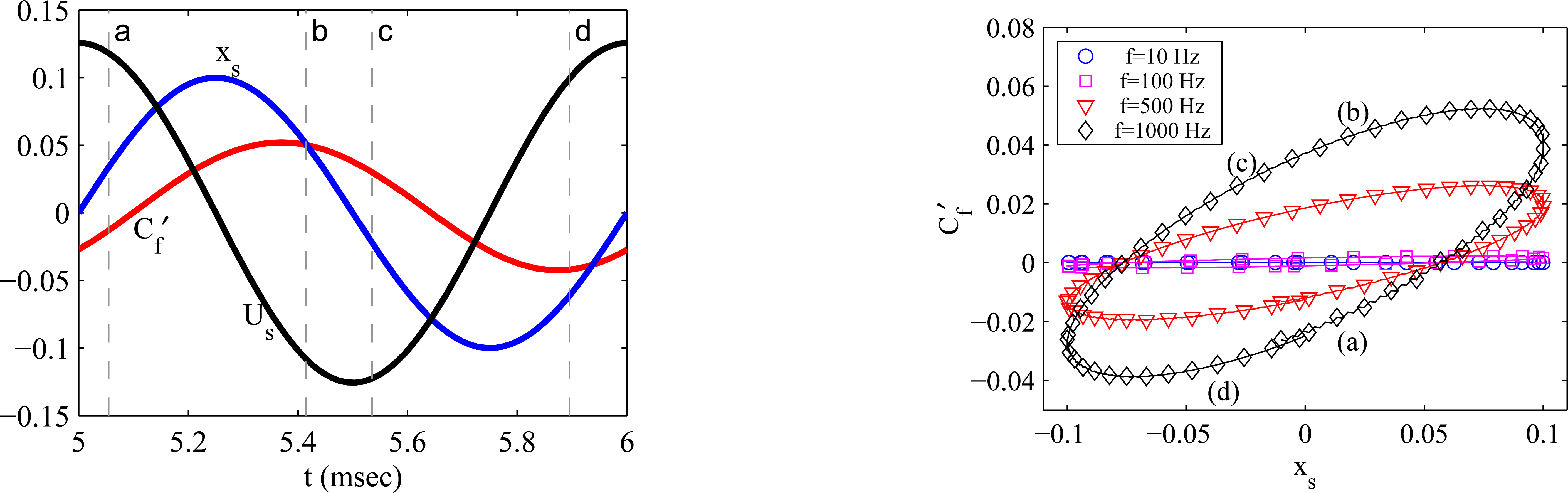
The analytical solution for an oscillating plane in a fluid can result in a phase shift of 45°(Landau/Lifschitz, “Fluid Mechanics”), so it is also expected that the shear stress will be out of phase with the sensor motion. Left side of figure 6 shows the sensor position and velocity along with the fluctuating skin friction. Here, the fluctuating skin friction lags significantly
The resultant effect of the phase difference between the sensor motion and the fluctuating shear stress is visualized by plotting
as a function of sensor position. Figure 6 shows this relationship for the sensor operating at several different frequencies. The positions in the cycle are again shown for reference. The effect of increasing the sensor oscillation frequency is to increase the magnitude of the fluctuating shear stress as would be expected since the sensor velocity scales with the frequency. This figure indicates that the sensor will experience asymmetric forcing when moving upstream and downstream. Both the asymmetry and strength of the shear force are characterized by the ellipses. One measure of the effect of the fluid on the oscillating sensor is given by the area contained within the ellipse.
Although the effect of varying the frequency on the resultant
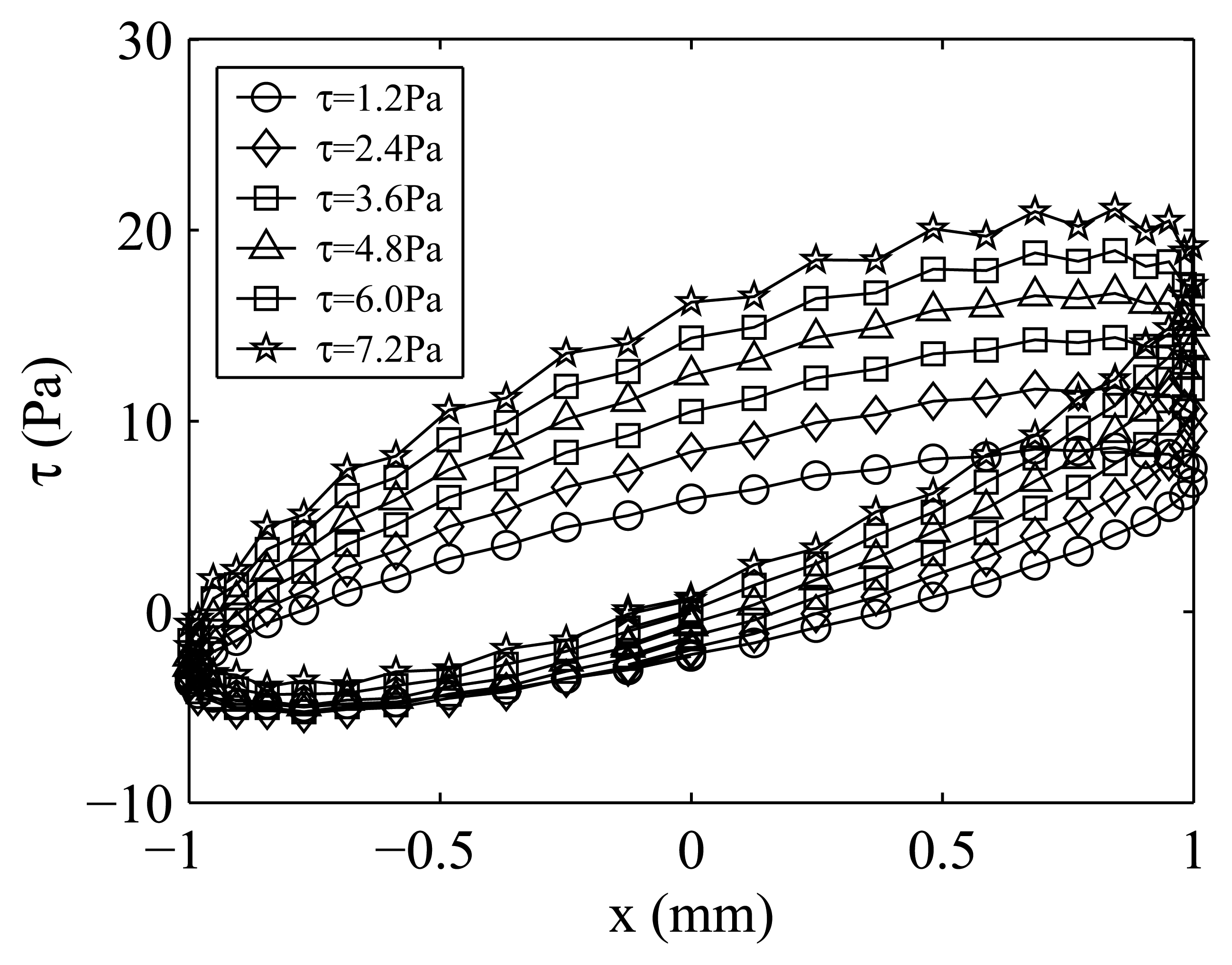
is important for designing the sensor, actual sensor operation is better visualized by varying the mean wall shear and observing the effect on the fluctuating wall shear. Figure 7 shows the fluctuating shear stress on the sensor surface for different mean shear stress levels. This figure shows that, as the mean shear is increased, the tilt and size of the ellipse increases indicating that the fluctuating shear force on the sensor is changing as the mean shear changes. Note that the upward migration of the curves occurs because the total shear is plotted and the mean shear is increasing. If the increasing mean shear produces a sufficient change, a response in the sensor model should be observed. These results indicate that a sensor oscillating near resonance should be sensitive to changes in wall shear stress and that the mechanism responsible is the finite lag time associated with the fluid.
5.2. Coupled Fluid/Mechanical Model Results
5.2.1. Sensor Response Behavior
A coupled fluid/mechanical model of the sensor is necessary to completely understand its performance. Such a model can be used to predict sensor performance as well as to guide the design of future sensors.
For the simulations performed here, sensor properties that corresponded to the prototype shown in figure 2 are used (m=0.537g, b=3.36 g/s, k=1250 N/m, and Fm=7.46 mN). Since this sensor has already been shown to work, [14] it provides a case for which the model should succeed.
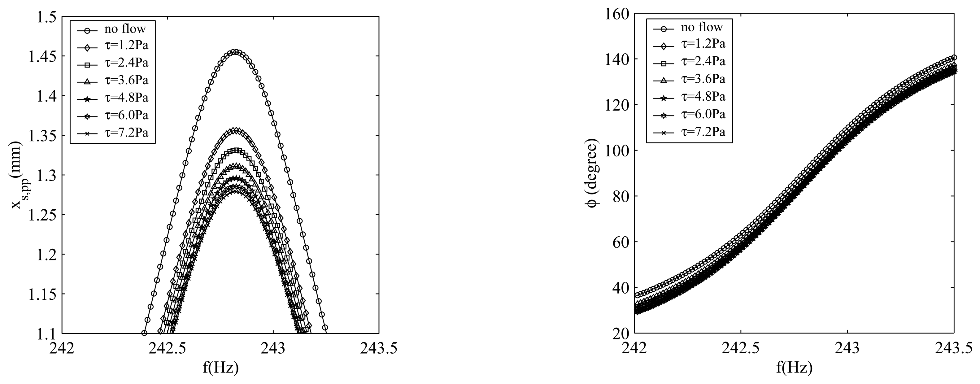
To determine the sensitivity of the sensor to different driving frequencies, all parameters but the frequency are held constant and the frequency is varied over a range bracketing resonance. This process is repeated for several different evenly spaced wall shear stress levels. The results are shown in figure 8 where both the amplitude and phase response are shown. Although only a portion of the resonance peak is shown, it is clear that the peak is very narrow, a characteristic typical of a high-Q system. The peak-to-peak amplitude shown in figure 8 decreases monotonically with increasing shear stress. The increment of amplitude decrease is reduced at higher wall shear stress levels. The large jump from flow off to the first shear level indicates that sensitivity remains to measure lower shear levels - perhaps much lower. In contrast, the collapse of the curves at the higher shear levels indicates a saturation of the sensor's response. The phase at which the peak resonance is observed changes little with increasing shear, although some shift downward and to the right is evident in figure 8. This is important because, if the sensor is operated at fixed frequency, its position relative to the resonance peak is essentially constant.
5.2.2. Sensor Sensitivity
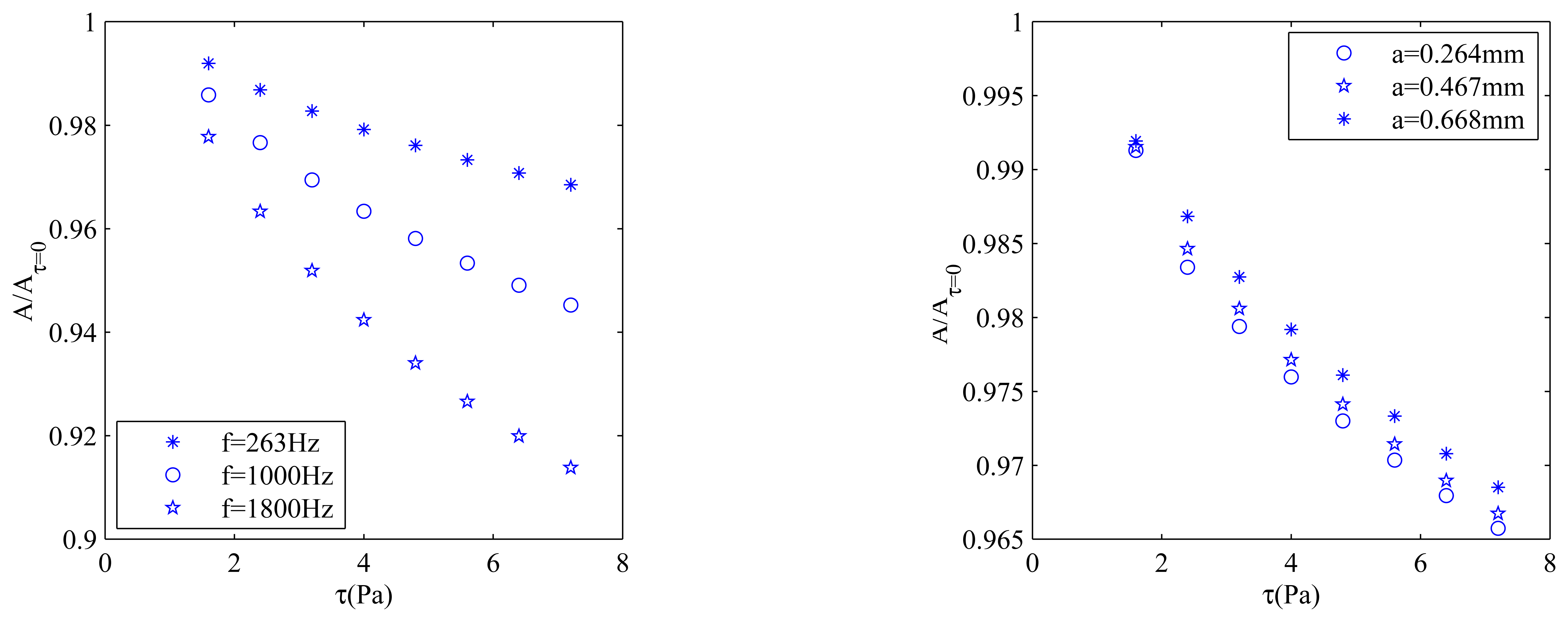
Numerical simulations corresponding to fixed frequency-variable oscillating amplitude and fixed amplitude-variable resonant frequency were performed. For the fixed frequency simulations, a frequency of 263 Hz was used. Three different oscillating amplitudes, a = 0.264 mm, a = 0.467 mm, a = 0.668 mm, were chosen to keep the oscillating amplitudes in the linear elastic range of the sensor material. To investigate frequency effects, an oscillating amplitude of a = 0.264 mm was chosen and three different oscillating frequencies, f = 263 Hz, f = 1000 Hz, f = 1800 Hz, were simulated. Here, the parameter selections for frequency influences did not consider the sensor structure and material properties, which are not possible to have several resonant frequency for a specific sensor element structure. So this simulation is exaggerated in some extend.
The influence of sensor amplitude on the static calibration curve in a flat plate boundary layer flow is shown in figure 9 for several shear levels, where A represents the peak-to-peak amplitude of the sensor at different shear stress levels, AT=0 represents the peak-to-peak amplitude of the sensor at zero shear stress level, and τ is defined as mean shear stress acting on the sensor. Figure 9 indicates that a smaller sensor oscillating amplitude has a little bit more sensitivity. This can be explained by considering that, when the sensor amplitude is decreased, the driving force becomes much smaller, and the resulting driving force is more comparable with shear stress force. The influence of sensor frequency on the static calibration curve in the same boundary layer flow as figure 9 was determined and is shown in figure 9. From the figure, it is evident that increasing the resonant frequency will increase the sensor sensitivity. When the resonant frequency increases, the fluctuating shear stress due to the sensor motion will increase significantly due to the high sensor velocity. Higher resonant frequency sensors will be pursued in the future because there is a significant sensor sensitivity increase with increasing resonant frequency(resonant frequency is related to sensor mass and stiffness).
6. Future Work
Although the existing sensor has been numerically investigated its related behavior, it requires further characterization to develop into a functioning sensor. Dynamic response of this type of shear stress sensor is still need further investigation. At the same time, in order to experimentally investigate scale effects, small size dynamic resonant shear stress sensor experiments will be the future developing direction. In addition, MEMS sensor should be developed to take advantage of the small size possible with micro-machining technologies. How to drive a MEMS sensor element and how to make a MEMS sensor element with high resonant frequency are also a big challenge work.
7. Conclusion
In order to understand how and why the dynamic resonant sensor works, a two-dimensional unsteady boundary layer code has been developed. This code was a minimum level analysis in order to determine the time-dependent shear stress due to the sensor motion and, it was much more time-efficient than running a general time-dependent flow solver. In the two-dimensional unsteady boundary layer flow model, the gap effects between dynamic sensor and the non-moving surface have been neglected. There is expected to be some damping effect from this region, but it has been neglected to simplify the calculations.
The development of a coupled fluid mechanical model is complete, which was the primary objective of the work discussed here. The model shows that the mechanism responsible for the successful operation of the sensor is the finite response time of the fluid to the oscillating sensor surface and is characterized by the integral of the fluctuating shear stress with respect to sensor position. Simulations based on the properties of a prototype sensor indicate that the sensor is sensitive to shear stress when operating near resonance, although the response is non-linear. These results suggest that the concept of a dynamic resonant sensor is sound.
Acknowledgments
The authors would like to thank Michael Scott, Eddie Adcock, and Sateesh Bajikar of NASA-Langley Research Center. Their participation under Memorandum of Agreement SAA1-646 has been helpful to the success of this project.
References
- Winter, K.G. An outline of the techniques available for the measurement of skin friction in turbulent boundary layers. Progress in Aerospace Sciences 1977, 18, 1–57. [Google Scholar]
- Haritonidis, J. H. The measurement of wall shear stress. Advances in Fluid Mechanics 1989. [Google Scholar]
- Naughton, J.W.; Sheplak, M. Modern developments in shear stress measurement. Progress in Aerospace Sciences 2002, 38, 515–570. [Google Scholar]
- Schmidt, M.A.; Howe, R.T.; Senturia, S.D.; Haritonidis, J.H. Design and calibration of a micro-fabricated floating-element shear-stress sensor. Transactions of Electron Devices 1988, 35, 750–757. [Google Scholar]
- Desai, A.V.; Haque, M. A. Design and fabrication of a direction sensitive mems shear stress sensor with high spatial and temporal resolution. J. Micromech. Microeng. 2004, 14, 1718–1725. [Google Scholar]
- Ng, K.; Shajii, J.; Schmidt, M.A. A liquid shear-stress sensor using wafer-bonding technology. Journal of Microelectricalmechanical Systems 1992, 1, 931–934. [Google Scholar]
- Barlian, A. A.; Parka, S.-J.; Mukundana, V.; Pruitta, B. L. Design and characterization of microfab-ricated piezoresistive floating element-based shear stress sensors. Sensors and Actuators A:Physical 2007, 134(1), 77–87. [Google Scholar]
- Li, Y.; Nishida, T.; Arnold, D.; Sheplak, M. Microfabrication of a wall shear stress sensor using side-implanted piezoresistive tethers. Proceeding of SPIE 14th Annual International Symposium on Smart Structures and Materials, San Diego, CA; 2007. [Google Scholar]
- Padmanabhan, A.S.M.; Breuer, K.S.; Schmidt, M.A. Micromachined sensors for static and dynamic shear stress measurements in aerodynamic flows. Transducers 1997. [Google Scholar]
- Tseng, F.; Lin, C. Polymer mems-based fabry-perot shear stress sensor. IEEE SENSORS Journal 2003, 3(6), 812–817. [Google Scholar]
- Pan, T.; Hyman, D.; Mehregany, M.; Reshotko, E.; Garverick, S. Microfabricated shear stress sensors, part 1: design and fabrication. AIAA Journal 1999, 37, 66–72. [Google Scholar]
- Zhe, J. Z.; Farmer, K. R.; Modi, V. A mems device for measurement of sking friction with capacitive sensing. Porceedings of IEEE MEMS 2002. [Google Scholar]
- Horowitz, S.; Chen, T.; Chandrasekaran, V.; Tedjojuwono, K.; Nishida, T.C.L.; Sheplak, M. Micromachined geometric moiré interferometric floating element shear stress sensor. AIAA 2004-1042 2004. [Google Scholar]
- Armstrong, W. D.; Singhal, A.; Naughton, J. W. A dynamic resonant wall shear stress sensor. AIAA Paper 2004, 2004–2608. [Google Scholar]
- Panton, R. L. Incompressible FlowWiley, second edition; 1996. [Google Scholar]
- Anderson, Dale A.; Tannehill, J.o.C.; Pletcher, R.H. Computational fluid mechanics and heat transfer; McGraw-Hill: New York, 1984. [Google Scholar]
- Keller, H.B. Numerical methods in boundary-layer theory. Annual Review of Fluid Mechanics 1978, 10, 417–433. [Google Scholar]
- Cebeci, T.; Cousteaux, J. Modeling and Computation of Boundary-Layer Flows; Springer, 1999. [Google Scholar]
- Cebeci, P. B. T.; Whitelaw, J. H. Engineering calculation methods for turbulent flows; Academic press, 1981. [Google Scholar]
Figure 1.
Schematic of the dynamic resonant wall shear stress sensor showing important components and parameters.
Figure 1.
Schematic of the dynamic resonant wall shear stress sensor showing important components and parameters.

Figure 2.
Prototype dynamic resonant shear stress sensor: image of the sensor and solid model of the sensor.
Figure 2.
Prototype dynamic resonant shear stress sensor: image of the sensor and solid model of the sensor.
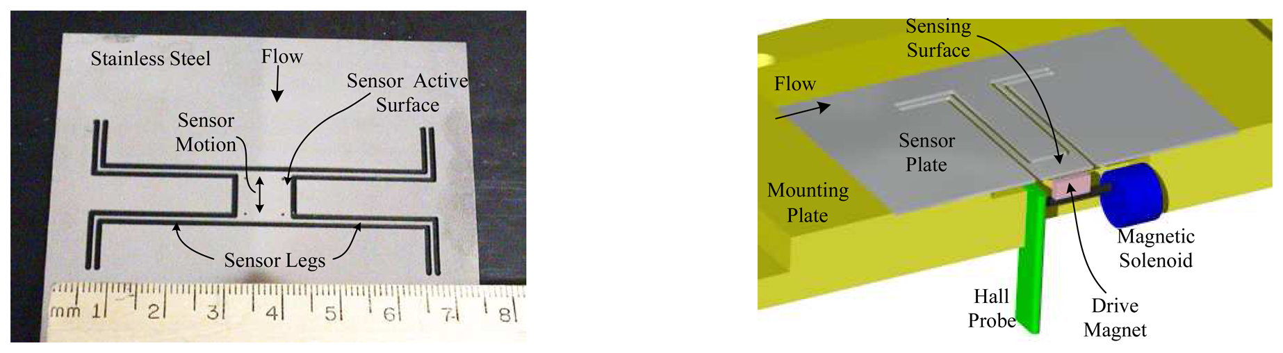
Figure 3.
zig-zag scheme.

Figure 4.
Velocity distributions in region just above sensor: velocity distribution and velocity distribution with the laminar boundary layer velocity distribution subtracted. The conditions for this case are Re=50000, a*=0.02, St=10, and Hr=0.02.
Figure 4.
Velocity distributions in region just above sensor: velocity distribution and velocity distribution with the laminar boundary layer velocity distribution subtracted. The conditions for this case are Re=50000, a*=0.02, St=10, and Hr=0.02.

Figure 5.
Skin friction distribution along flat plate with sensor: (a) mean skin friction, (b) mean skin friction with laminar boundary layer skin friction removed, and (c) rms Skin friction. The conditions for this case are Re=50000, a*=0.02, St=10, and Hr=0.02.
Figure 5.
Skin friction distribution along flat plate with sensor: (a) mean skin friction, (b) mean skin friction with laminar boundary layer skin friction removed, and (c) rms Skin friction. The conditions for this case are Re=50000, a*=0.02, St=10, and Hr=0.02.

Figure 6.
Time record of sensor position and unsteady skin friction experienced by the sensor and unsteady skin friction on sensor surface for different actuation frequencies. Provide conditions here. The conditions for this case are Re=50000, a*=0.02.
Figure 6.
Time record of sensor position and unsteady skin friction experienced by the sensor and unsteady skin friction on sensor surface for different actuation frequencies. Provide conditions here. The conditions for this case are Re=50000, a*=0.02.
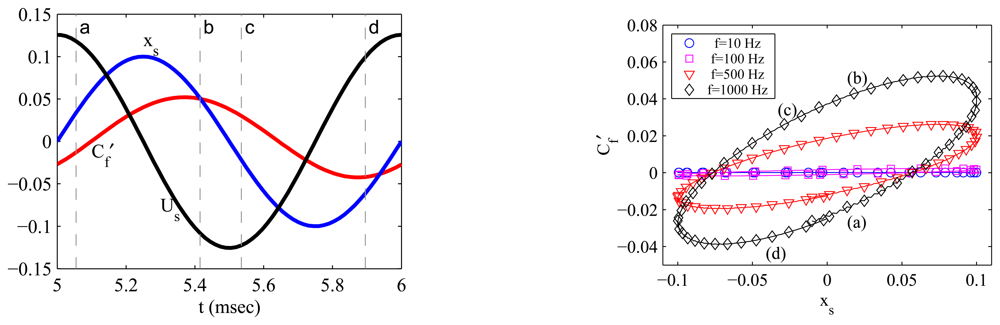
Figure 7.
Unsteady skin friction on sensor surface for different wall shear stress levels. The conditions for this case are f=240 Hz and a*=0.14.
Figure 7.
Unsteady skin friction on sensor surface for different wall shear stress levels. The conditions for this case are f=240 Hz and a*=0.14.

Figure 8.
Response of a dynamic resonant shear stress sensor in a laminar boundary layer: (a) amplitude response, and (b) phase response. The condition held constant for this case is a* = 0.14, and the sensor properties were m=.537 g, k=1250 N/m, b=3.36 g/s, and Fm=7.46 mN.
Figure 8.
Response of a dynamic resonant shear stress sensor in a laminar boundary layer: (a) amplitude response, and (b) phase response. The condition held constant for this case is a* = 0.14, and the sensor properties were m=.537 g, k=1250 N/m, b=3.36 g/s, and Fm=7.46 mN.

Figure 9.
Amplitude and frequency influences on the sensor sensitivity.


| Quantity | Expression |
|---|---|
| Reynolds Number(Re) | UL/ν |
| Strouhal Number(St) | fLs/U |
| Amplitude Ratio(a*) | a/Ls |
| Penetration Depth Ratio(Y*) | ν1/2/Lsf1/2 |
| Sensor/Flow Length Scale Ratio(L*) | Ls/L |
| Hummer Number(Hr) | τ0/ρν1/2f3/2Ls |
© 2008 by MDPI (http://www.mdpi.org). Reproduction is permitted for noncommercial purposes.
Share and Cite
MDPI and ACS Style
Zhang, X.; Naughton, J.W.; Lindberg, W.R. Working Principle Simulations of a Dynamic ResonantWall Shear Stress Sensor Concept. Sensors 2008, 8, 2707-2721. https://doi.org/10.3390/s8042707
AMA Style
Zhang X, Naughton JW, Lindberg WR. Working Principle Simulations of a Dynamic ResonantWall Shear Stress Sensor Concept. Sensors. 2008; 8(4):2707-2721. https://doi.org/10.3390/s8042707
Chicago/Turabian StyleZhang, Xu, Jonathan W. Naughton, and William R. Lindberg. 2008. "Working Principle Simulations of a Dynamic ResonantWall Shear Stress Sensor Concept" Sensors 8, no. 4: 2707-2721. https://doi.org/10.3390/s8042707