Topographic Effects on the Surface Emissivity of a Mountainous Area Observed by a Spaceborne Microwave Radiometer

Abstract

A simulation study to understand the influence of topography on the surface emissivity observed by a satellite microwave radiometer is carried out. We analyze the effects due to changes in observation angle, including the rotation of the polarization plane. A mountainous area in the Alps (Northern Italy) is considered and the information on the relief extracted from a digital elevation model is exploited. The numerical simulation refers to a radiometric image, acquired by a conically-scanning radiometer similar to AMSR-E, i.e., flying at 705 km of altitude with an observation angle of 55°. To single out the impact on surface emissivity, scattering of the radiation due to the atmosphere or neighboring elevated surfaces is not considered. C and X bands, for which atmospheric effects are negligible, and Ka band are analyzed. The results indicate that the changes in the local observation angle tend to lower the apparent emissivity of a radiometric pixel with respect to the corresponding flat surface characteristics. The effect of the rotation of the polarization plane enlarges (vertical polarization), or attenuates (horizontal polarization) this decrease. By doing some simplifying assumptions for the radiometer antenna, the conclusion is that the microwave emissivity at vertical polarization is underestimated, whilst the opposite occurs for horizontal polarization, except for Ka band, for which both under- and overprediction may occur. A quantification of the differences with respect to a flat soil and an approximate evaluation of their impact on soil moisture retrieval are yielded.

1. Introduction

Spaceborne microwave radiometric observations of land are mainly determined by surface emissivity and temperature, especially at frequencies where the atmosphere is more transparent. If bare soil is considered, its emissivity at a given frequency depends on moisture, which influences the dielectric permittivity of a smooth surface [1], surface geometry (at wavelength scale i.e., roughness, and at resolution scale, i.e., topography) and, to a less extent, on composition and density. Over mountainous areas, which represent important targets within Earth remote sensing from satellites, especially for hydrological purposes, the relief effects must be carefully taken into account [2]. Moreover, at microwave frequencies, the highly inhomogeneous features of the mountainous scenario should be compared with the relatively large antenna footprints.

Large-scale relief effects on the upwelling brightness temperature (T_B) measured by a spaceborne radiometer are [2-3]: i) modification of the atmospheric contributions due to their dependence on the altitude of the emitting surface; ii) shadowing of the downwelling atmospheric radiation; iii) local modification of the observation angle with respect to a flat terrain, which may cause shadowing of the upwelling surface radiation; iv) rotation of the linear polarization plane. These effects imply an overall change of the apparent emissivity with respect to the surface characteristics that can affect the retrieval of bio-geophysical parameters, such as soil moisture.

The topography effects for microwave radiometry over land have been analyzed in a past investigation carried out by Mätzler and Standley [2]. They underlined that a weak attention was paid to this aspect before the publication of their study. However, they focused on one of the effects, i.e., the shadowing of sky radiation by the surrounding elevated terrain. According to their conclusions, a pixel illuminated by the radiation coming from neighbors located at higher altitude, increases its T_B with respect to a pixel which scatters atmospheric downward radiation only. The impact of the relief has been also considered in a brief report by Kerr et al. [3] and, recently, by Talone et al. [4]. Both studies concern the L band SMOS instrument using aperture synthesis. In [3], the level of topography influencing the radiometric signal is assessed. In [4], the relief has been accounted for in a SMOS End-to-End performance simulator, leading to a quantification of the variation of the local observation angle up to 55°, and to a warning on its possible impact.

The main objective of this study is the quantification of the effects of changes in local observation angle on the emitted component of the radiation measured by a satellite microwave radiometer observing a mountainous scene. In addition, we also aim at yielding an approximate evaluation of the impact of these effects on soil moisture retrieval. The interest in pursuing these goals is due to the fact that most of the algorithms developed to retrieve bio-geophysical parameters (such as soil moisture) assume that the Earth surface is flat, so that their applicability to mountainous areas may be questioned. A quantification of the relief effects on microwave radiometry is therefore useful for preliminary correcting radiometric data before applying retrieval algorithms tuned for flat terrains.

Here we focus on the modification of the local observation angle and the rotation of the plane of linear polarization, thus complementing the investigation accomplished in [2] for a complete analysis of the various effects of the large-scale surface geometry. For this purpose, we have exploited semi-empirical models for rough bare soil [5-6], a digital elevation model (DEM) of an Alpine region in Italy, and some simplifying assumptions concerning the radiometer antenna and its conical scanning (as in [2]) to simulate the T_B observed by an imaging radiometer. We have considered the Advanced Microwave Scanning Radiometer for the Earth Observing System (AMSR-E), i.e., an instrument flying at 705 km of altitude with an observation angle of 55° [7]. Focusing on the emitted component of upwelling T_B, reflection of the radiation due to the atmosphere or neighboring elevated surfaces (already treated in [2]) is not taken into account here. Our analysis starts from low frequencies (in particular, C and X bands, i.e., 6.925 and 10.65 GHz) for which, in the absence of rain, atmospheric effects can be neglected [8]. However, since at these frequencies the poor spatial resolution tends to smooth relief effects on surface emission, the latter are discussed for Ka band (36.5 GHz) too.

The work is organized as follows. Section 2 describes the simulation methodology, i.e., the procedure that we have adopted to compute the emissivity of each DEM point at the three AMSR-E frequency bands considered here and to simulate the radiometric observation. In section 3, the comparison between the synthetic T_B's obtained from the simulated image of the mountainous scene and those relative to a flat bare soil having the same characteristics (roughness, moisture, composition, etc.) is discussed. Section 4 draws the main conclusions.

2. Simulation Methodology

To simulate the radiometric observation of a mountainous area, we have firstly computed the local observation angle of each surface element of the DEM. Then, we have estimated the emissivity toward the satellite radiometer of a DEM element. To do this, we have selected two semi-empirical models that allow calculating the microwave surface emissivity as a function of the local observation angle and of the soil roughness parameters. Finally, the observation of the satellite radiometer has been simulated by assuming specific measurement geometry. For this purpose, we have evaluated the elements of the DEM comprised in the instantaneous field of view of the radiometer antenna and then we have estimated the antenna temperature. Hereafter, a description of the simulation methodology is given in detail.

2.1. Computation of the emissivity

We have focused our analysis on a mountainous area in the Alps (Northern Italy) and we have derived the topography from a DEM with a spatial resolution of 250×250 m. A matrix of 512×512 points, i.e., an area of 128×128 km has been considered. For each DEM element, the aspect and the slope angles have been extracted and the local surface normal has been determined. Then, the angle between the local surface normal and the radiometer pointing direction, i.e., the local observation angle θ_l, has been computed.

The electromagnetic models of the complex dielectric permittivity ε proposed by Dobson et al. [1], for C and X bands, and by Calvet et al. [9], for Ka band, have been adopted. Note that the former is valid within the 1.4 to 18 GHz region, whilst the latter is suitable for higher frequencies. We have computed ε for a terrain characterized by fairly standard values of volumetric moisture (0.30), dry soil density (1.3 g/m³) and soil temperature (296 K). The fractions of sand and clay have been assumed equal to 48.5% and 18.5%, respectively.

To calculate the surface emissivity, we have selected the model developed by Wegmüller and Mätzler [5] (hereafter denoted by WM model), since it is characterized by a wide range of applicability, both for frequencies and observation angles. A different model, derived from the measurements performed at the “Institut National de la Recherche Agronomique” (INRA) [6] (hereafter INRA model) and suitable for high frequencies, has been also used for the 36.5 GHz band. Bare terrains characterized by standard deviations of height (s) equal to 0.89 and 1.91 cm have been considered, as done in [6].

According to [5], the p-polarized emissivity of the soil (e_p), where p may be H (horizontal) or V (vertical) is given by:

$$e_H\left({\theta }_l\right)=1-\left(1-e_{0H}\right)exp[-{\left(ks\right)}^{\sqrt{0.10cos{\theta }_l}}]$$

(1a)

$$e_V\left({\theta }_l\right)=\{\begin{array}{ll}1-\left[1-e_H\left({\theta }_l\right)\right]{\left(cos{\theta }_l\right)}^{0.655}\hfill & {\theta }_l\le 60°\hfill \\ 1-\left[1-e_H\left({\theta }_l\right)\right]\left[0.635-0.0014\left({\theta }_l-60°\right)\right]\hfill & {\theta }_l>60°\hfill \end{array}$$

(1b),(1c)

In equations (1), (1−e_0H) denotes specular reflectivity (one minus emissivity) at H polarization and θ_l indicates the local observation angle.

The INRA model expresses the soil emissivity as [6]:

$$e_p\left({\theta }_l\right)=1-[1+e_{0p}\left({\theta }_l\right)\left(Q-1\right)-Q{e}_{0q}\left({\theta }_{li}\right)]exp[-h{cos}^N\left({\theta }_l\right)]$$

(2)

In Equation (2), p and q stand for either V or H polarization and Q, h and N are parameters depending on the type of terrain and on frequency. As suggested in [6], at Ka band, Q, h and N have been assumed equal to 0.33, 0.15 and 0.0, respectively, for s=0.89 cm and to 0.45, 0.62 and 0.5, respectively, for s=1.91 cm.

Figure 1 shows the trend of the emissivity versus the observation angle, as predicted by the two models. It can be noted that the emissivity foreseen by the INRA model for the 36 GHz band is smaller than the emissivity predicted by the WM model (at the same frequency). The former presents a higher sensitivity to the observation angle, with a sharper decrease in correspondence to higher angles. Furthermore, for s=0.89 cm, the appearance of the Brewster effect can be observed for the INRA model. We point out that the consideration of two emissivity models, presenting different sensitivities to the observation angle, aims at assessing the generality of the results. A comparison of these models or their validation is beyond the scope of this study.

The emissivity of each element of the DEM, as a function the local observation angle, has been firstly calculated by applying equations (1) and (2). Then, we have determined the angle between the polarization basis vectors in the global coordinate system (related to the direction of observation) and in the local coordinate system (related to the surface element), that is the rotation angle of the polarization plane α (see [10] for details). The emissivity in the global frame is expressed by [2]:

$$e_p^{\prime }\left({\theta }_l,\alpha \right)=e_p\left({\theta }_l\right){cos}^2\alpha +e_q\left({\theta }_l\right){sin}^2\alpha$$

(3)

This rotation causes a decrease of the emissivity at V polarization and an increase at H polarization, i.e., a change in the observed polarization.

2.2. Simulation of a radiometric observation

We have simulated the radiometric image for three frequency bands: 6.925, 10.65 and 36.5 GHz. A conically-scanning sensor observing the Earth at θ =55°, from an altitude R=705 km and with a track from North to South along the central column of the DEM matrix has been assumed. A pixel spacing of 10×10 km has been supposed, with the following spatial resolutions: 75×43, 51×29 and 15×8 km for the, 6-, 10-, and 36-GHz bands, respectively [7]. The upper panel of Figure 2 shows the simulation of the scan at 36 GHz. Note that in the area that we have considered for this exercise (128×128 km) 11 (in the direction of the radiometer track) by 13 radiometric pixels are included. Obviously, for the lower frequencies, this number is smaller.

We have determined the elements of the DEM comprised in every radiometric pixel, i.e., in the instantaneous field of view (IFOV) of the radiometer antenna, in a fairly approximate way. Denoting by σ_x and σ_y the semiaxes of the ellipse representing the radiometric IFOV, by m_x and m_y the coordinates of the IFOV center, and by γ the azimuthal step of the sensor scan (Figure 2, upper panel), an element of the DEM, whose central points coordinates are (x, y), is contained in the elliptic IFOV if the following inequality is satisfied:

$$\frac{{(x-m_x)}^2}{{\sigma }_x^2}+\frac{{(y-m_y)}^2}{{\sigma }_y^2}+tan(2\gamma )\frac{({\sigma }_x^2-{\sigma }_y^2)}{{\sigma }_x^2{\sigma }_y^2}(x-m_x)(y-m_y)\le 1$$

(4)

Once the number N of DEM elements included in a given elliptic IFOV has been identified, the antenna temperature must be computed. For this purpose, some simplifying assumptions about the radiometer antenna have been done. We have supposed that the antenna is characterized by major lobe efficiency η_ml equal to 1 and by a constant directivity D within the major lobe. A constant distance R between the radiometer and every facet of the DEM has been assumed. Let us observe Figure 2, lower panel. The area A of a DEM element refers to a projection on the horizontal plane, whereas the actual area of a tilted facet is given by (A/cosβ_i), where β_i is the slope angle of the i-th element of the DEM, whose local angle is θ_li. Therefore, indicating by T_Bi the brightness temperature of the element (i.e., the emissivity multiplied by the surface temperature, assumed equal to 296 K in this exercise), the antenna temperature T_A, equal to the major lobe temperature with the above simplifications, can be expressed by:

$$T_A=\frac{\text{∑}_{i=1}^N{T}_{Bi}D{\Omega }_i}{\text{∑}_{i=1}^{N}D{\Omega }_i}=\frac{\text{∑}_{i=1}^N{T}_{Bi}D\frac{Acos{\theta }_{li}}{R^{2}cos{\beta }_i}}{\text{∑}_{i=1}^{N}D\frac{Acos{\theta }_{li}}{R^{2}cos{\beta }_i}}=\frac{\text{∑}_{i=1}^N{T}_{Bi}\frac{cos{\theta }_{li}}{cos{\beta }_i}}{\text{∑}_{i=1}^N\frac{cos{\theta }_{li}}{cos{\beta }_i}}$$

(5)

where Ω_i is the solid angle under which the i-th facet is observed by the radiometer, which is equal to (Acos θ_li/R²cosβ_i) [2]. According to Equation (5), the antenna temperature is given by the average of the brightness temperatures of the surface facets included in the antenna IFOV weighted by the ratio between the cosines of the local and the slope angles.

3. Results

The histogram of the normalized occurrences (NO) of the local observation angle in the considered Alpine region is shown in the upper panel of Figure 3. It can be observed that the distribution is fairly spread and that some occurrences at -10° are present. The latter actually correspond to angles greater than 90° that are not visible by the radiometer. The facets of the DEM with θ_l>90° do not contribute to the upwelling T_B. It is worth mentioning that the mean value of the visible local angles is 56.4°, greater than the nominal one (55°).

The histograms of the emissivity at 6.925 GHz for a bare soil with s=0.89 cm, computed by applying the WM model and Equation (3), are shown in the central and bottom panels of Figure 3 for H and V polarizations, respectively. It can be noted that the histogram for V polarization is narrower than the histogram for H polarization. This is due to the less sensitivity to the observation angle presented by the former (Figure 1, left panel).

The analysis of the results of our simulation is based on the comparison between the antenna temperature expressed by Equation (5) and the signal due to the emission of a flat terrain having the same characteristics. This signal is given by the emissivity computed by substituting the radiometer nominal observation angle (55°) instead of θ_l in equations (1) and (2), multiplied by the soil temperature (296 K). The objective of this comparison is the quantification of the errors, due to the emitted component of the observed radiation, caused by the modification of the local observation angle. As mentioned, we start from C and X bands since they are not affected by the atmosphere.

3.1. C and X bands

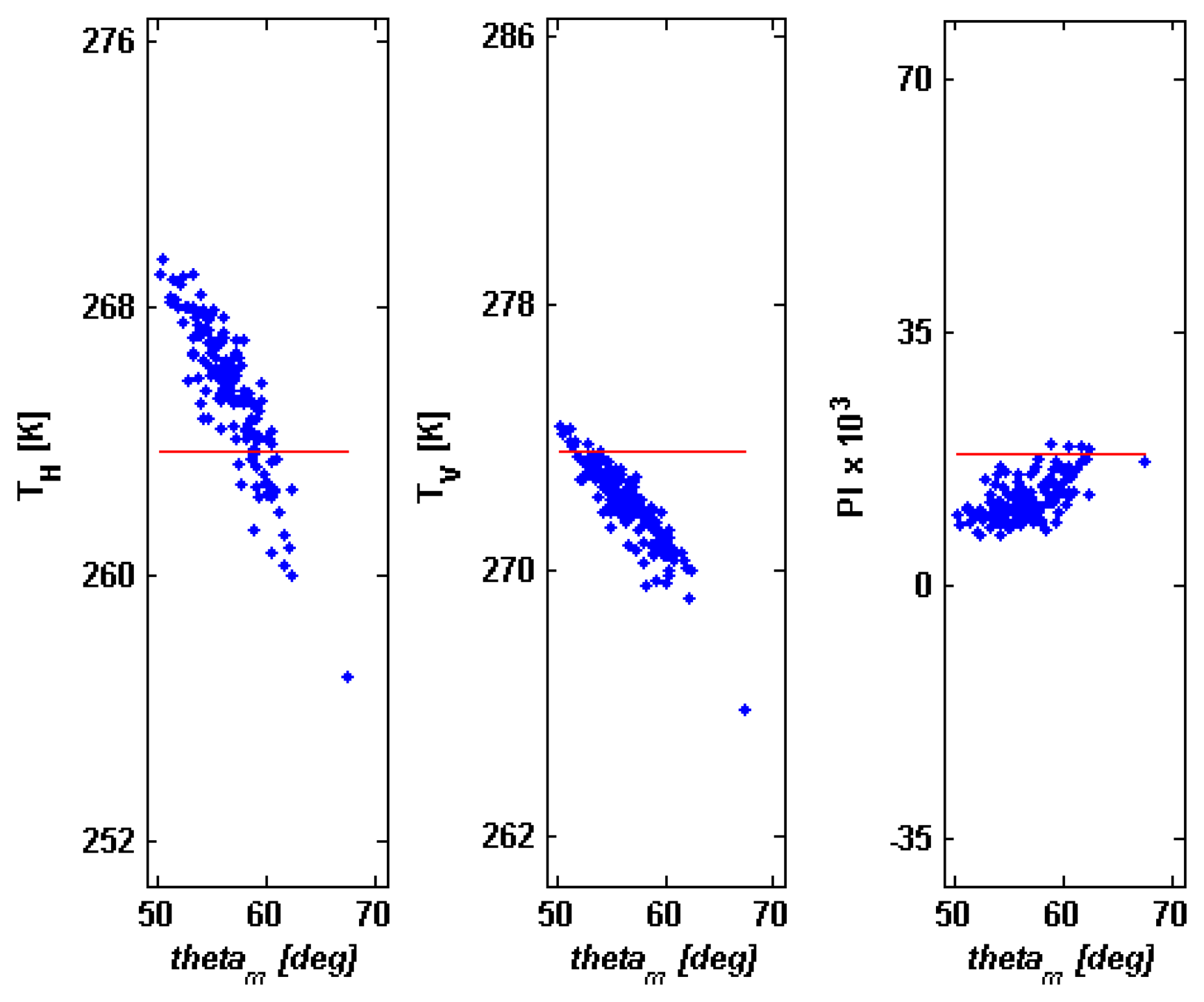
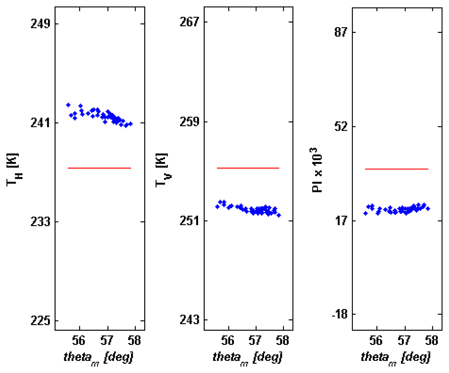
For C and X bands, only the WM emissivity model has been used. Figure 4 shows, for the 6 GHz band and for s=0.89 cm, the values of the various T_A 's that we have obtained through our simulation procedure, versus the average observation angle θ_m of a radiometric IFOV, that is the mean value of θ_li 's inside the antenna footprint. Left panel concerns H polarization (T_H), central panel V polarization (T_V). The polarization index (PI), equal to

$$PI=\frac{T_V-T_H}{T_V+T_H},$$

(6)

is also displayed in the right panel of Figure 4 (scaled by factor of 10³ for the sake of representation clarity). The values obtained for a flat terrain are also shown (red solid lines: T_Hflat, T_Vflat, PI_flat).

Table 1. Statistics of ΔT_H, ΔT_V and ΔPI at 6 GHz (WM model) for a bare surface with s=0.89 cm.

	ΔTH (K)	ΔTV (K)	ΔPI ×103
mean	4.16	-3.31	-15.20
std. dev.	0.39	0.24	0.81
max	5.10	-2.70	-13.58
min	3.49	-3.79	-16.77

quantifies the result reporting, for the 6 GHz band, the statistics of the differences between the T_A 's, i.e., of ΔT_H=T_H−T_Hflat, ΔTV=T_V−T_Vflat and of ΔPI= PI−PI_flat.

Figure 4 suggests that T_V and PI are always underestimated, whilst the opposite occurs for T_H. The maximum decrease of T_V is equal to 3.79 K and the maximum rise of T_H is 5.10 K (Table 1). To explain these results, we have to consider that three factors contribute to the variation of T_A with respect to that measured over a flat terrain [see Equation (5)]: i) the dependence of T_Bi on the local angle θ_li; ii) the dependence of Ω_i on the weighting quantity (cosθ_li/cosβ_i); iii) the rotation of the polarization plane. We can analyze these factors separately.

The modification of the local observation angle tends to lower the emissivity, especially at H polarization, which, as previously underlined, is more sensitive to this parameter. By neglecting both depolarization and weighting, the mean values of ΔT_H and ΔT_V at C band would be in the order of −6 K and −4 K, respectively, instead of 4.16 K and −3.31 K (Table 1). This is due to the presence within the antenna footprint of facets with large θ_li whose impact is fairly strong, because of the decrease of the emissivity with the rise of the observation angle (Figure 1, left panel). Furthermore, some facets are not visible by the radiometer, as previously pointed out.

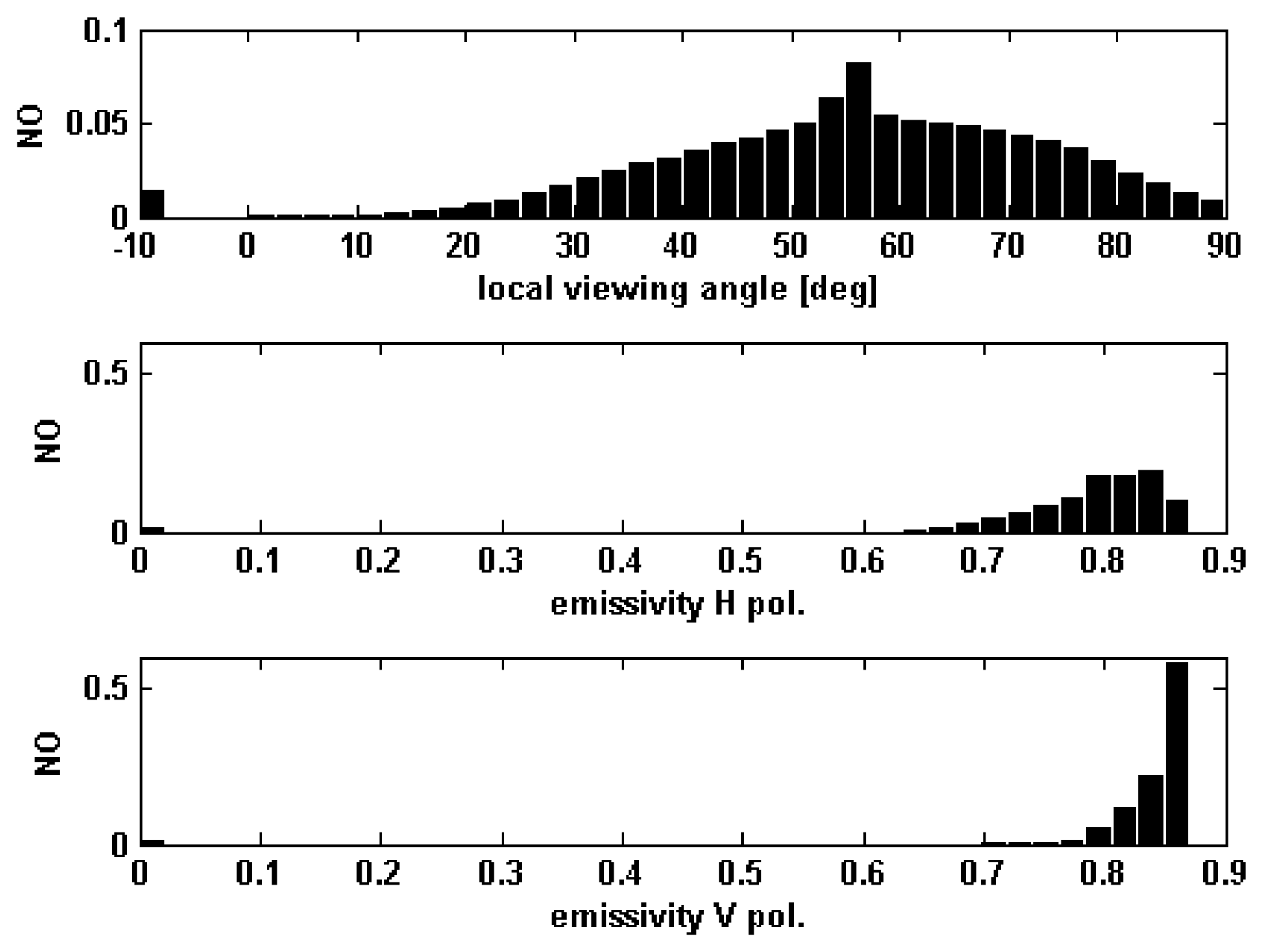
Regarding the impact of the beam weighting, due to the presence of the term (cosθ_li/cosβ_i) in Equation (5), for a flat terrain we would have cosθ_li=cos(55°) and cosβ_i=1 for all the elements of the DEM, so that Equation (5) would reduce to a simple average of T_Bi 's over the number of facets within the IFOV. For a mountainous scene, the weighting gives rise to an increase of T_A with respect to a simple average. This is due to the fact that the facets with the highest emissivity are those whose θ_li is small (Figure 1, left panel), i.e., the surfaces that are almost orthogonal to the radiometer direction of observation (Figure 2, lower panel). Since for these facets (cosθ_li /cosβ_i) is high, they appear to the radiometer under a large solid angle Ω_i [see Equation (5)]. In other words, the facets that weight most in Equation (5) are those characterized by high T_Bi, thus implying an overall increase of T_A. This increase is more evident for T_H, being smaller than T_V. Finally, the rotation of the polarization plane produces a coupling between the vertically and horizontally polarized emissivities [see Equation (3)] that implies a rise of T_H and a lowering of T_V.

We can now explain the results of Figure 4 and Table 1. The decrease of the emission of a radiometric pixel due to the change in the local angle is contrasted by the beam weighting (especially for H polarization), whilst the rotation of the polarization plane may enlarge (V polarization) or attenuate (H polarization) the lowering of T_A. Consequently, T_V and PI are always underestimated and T_H is overpredicted.

The differences (bias as well as standard deviation) quantified in Table 1 may affect the retrieval of bio-geophysical parameters, such as soil moisture, based on inversion algorithms tuned for flat terrains. To give an evaluation of the impact of these errors on estimates of soil moisture content (SMC), we have carried out a simple inversion of the forward model in which all the characteristics of the terrain specified at the beginning of Section 2 (standard deviation of height, dry soil density, fractions of sand and clay, etc.) are supposed known except SMC. Moreover, an angle of 55° (i.e., the radiometer nominal observation angle) is assumed. From the C band emissivities at H polarization (e_H) computed with our simulation procedure (i.e., the T_H 's divided by 296 K), we have determined the corresponding specular emissivities e_0H through equation (1a). Then, we have inverted the Fresnel equation to calculate the dielectric constant of the k-th radiometric pixel ε as done in [7]:

$${\varepsilon }_k={sin}^{2}55°+{\left[cos55°\frac{-1-\sqrt{\left(1-e_{0Hk}\right)}}{-1+\left(1-e_{0Hk}\right)}\right]}^2$$

(6)

Finally, we have fitted the model of Dobson et al. [1] to retrieve SMC. The histogram of the estimated SMC's is shown in Figure 5. The SMC values have to be compared with 0.3, which, as mentioned at the beginning of Section 2, is the nominal SMC for which the simulation has been accomplished. It can be inferred that neglecting the modification of the observation angle (i.e., considering a constant angle of 55°) leads to an underestimation of SMC, due to the overestimation of e_H. The mean value of the retrieved SMC is 0.24.

The results for X band, s=0.89 cm, are quantified in

Table 2. Statistics of ΔT_H, ΔT_V and ΔPI at10 GHz (WM model) for a bare surface with s=0.89 cm.

	ΔTH (K)	ΔTV (K)	ΔPI ×103
mean	3.65	-2.79	-12.79
std. dev.	0.56	0.37	0.97
max	5.06	-1.76	-10.48
min	2.68	-3.59	-14.98

. The dynamic range and the standard deviation are slightly larger with respect to C band because of the higher spatial resolution of the X band radiometric pixel that reduces the smoothing effect due to antenna beamwidth integration.

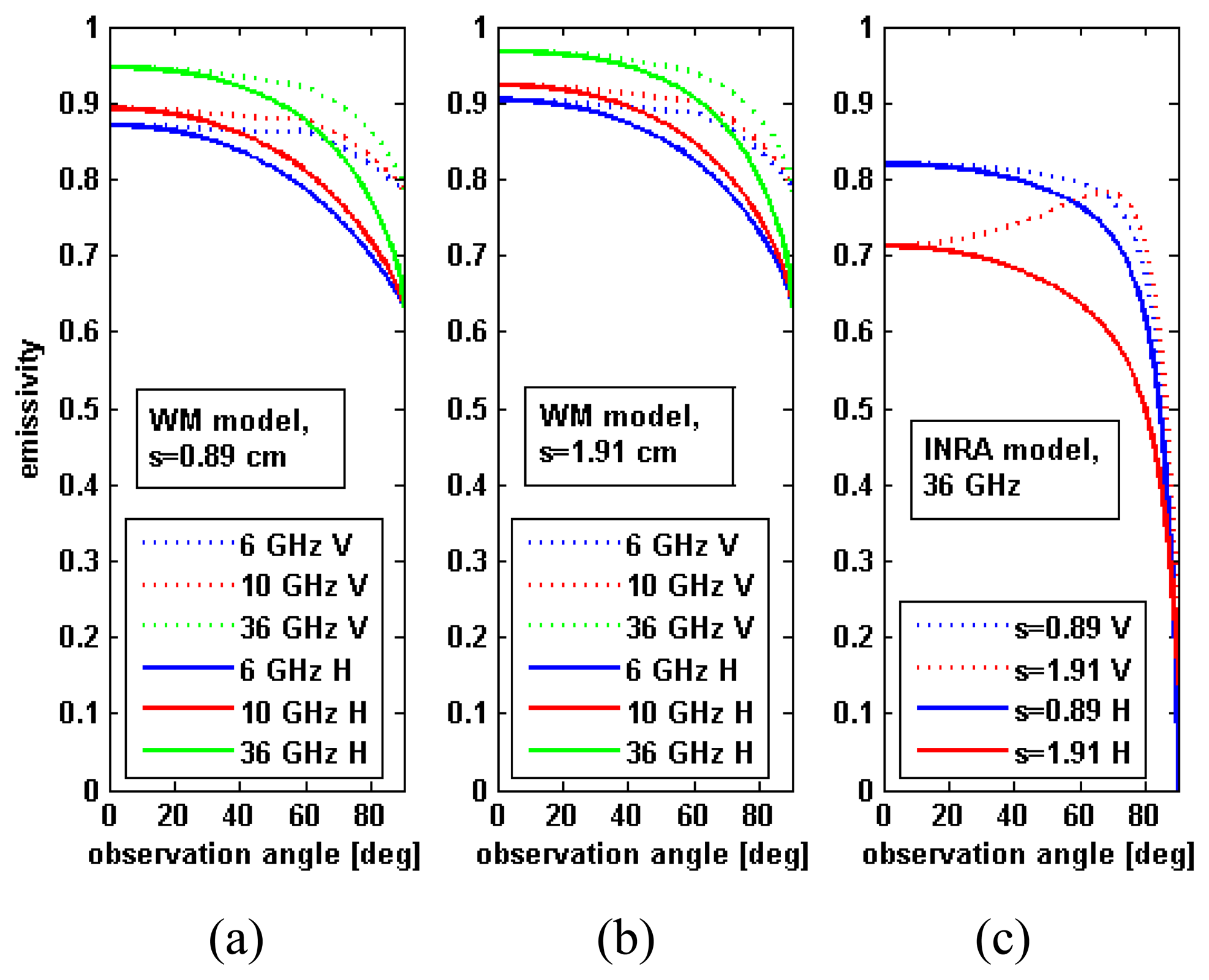
By observing left and central panels of Figure 1, it can be noted that the sensitivity of the emissivity to the observation angle is fairly similar, so that the results achieved for s=0.89 cm do not substantially change for s=1.91 cm and the explanation yielded above on the effects of the three factors on T_A still applies. The mean values of ΔT_H, ΔT_V and ΔPI obtained for the latter case are reported in

Table 3. Mean values of ΔT_H, ΔT_V and ΔPI for s=1.91 cm at C and X bands (WM model).

	ΔTH (K)	ΔTV (K)	ΔPI ×103
6 GHz	3.29	-2.54	-11.42
10 GHz	2.77	-2.09	-9.31

. The magnitude of the biases is slightly smaller with respect to the case of a less rough terrain.

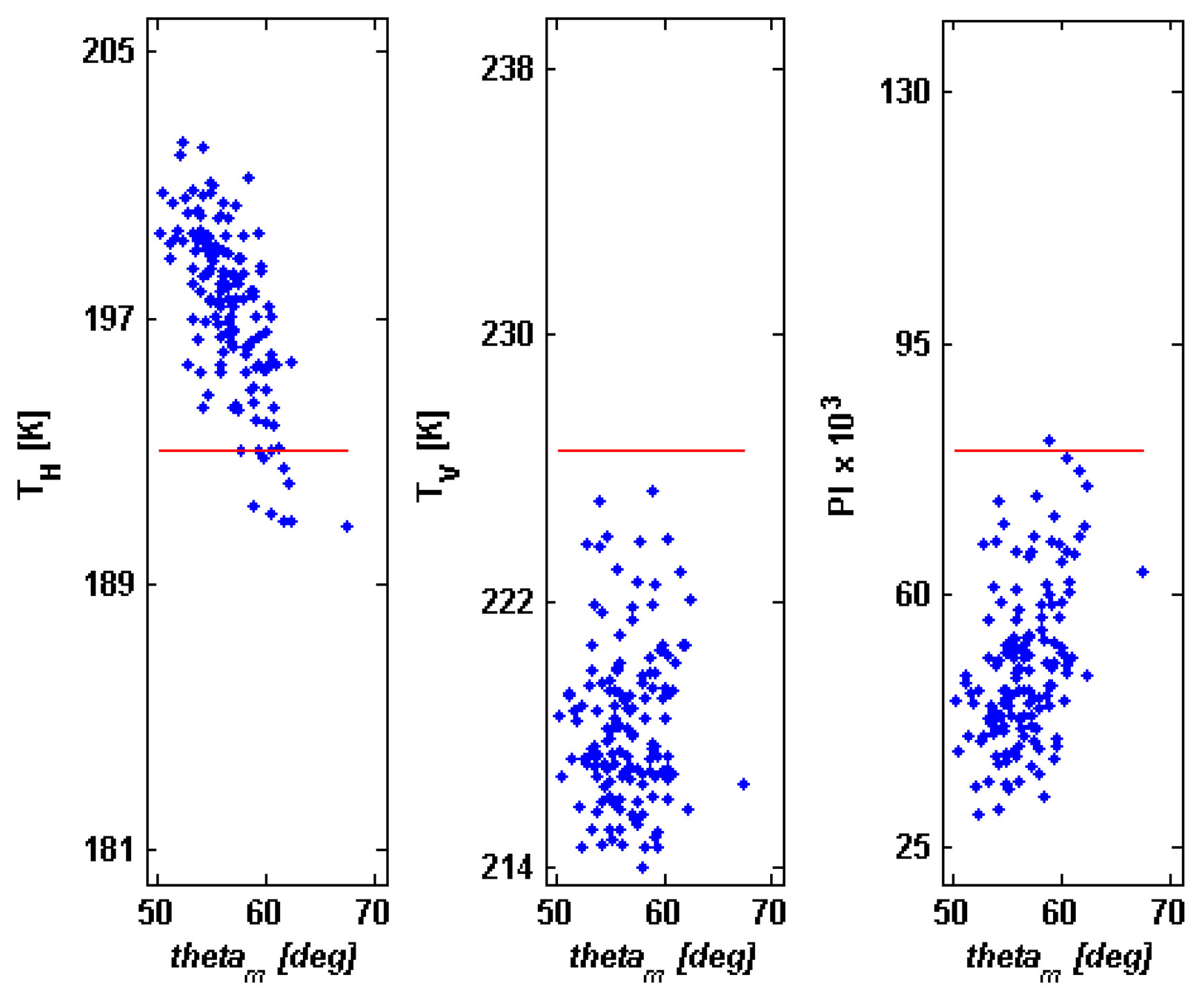
3.2. Ka band

Figure 6 is the analogous to Figure 4, but for the 36.5 GHz band (WM model, s=0.89 cm). First of all, it is understood that, in this case, actual measurements at Ka band are affected by the atmosphere. Limiting ourselves to the emission term, the analysis of Ka band allows us to better single out the topography effect and its dependence on local observation angle, since the smoothing effect of the low-resolution radiometric pixel noted for C and X bands is reduced. The general overestimation of T_H and underprediction of T_V and PI are confirmed. The clearest differences with respect to C band are represented by the increase of the correlation between T_A and θ_m, by the widening of the range of θ_m and by the increase of both the dynamics and the standard deviation of T_A. Furthermore, some situations in which T_H is underpredicted and few cases (small θ_m, in the order of 50°) in which T_V is slightly greater than T_Vflat occur.

Table 4. Statistics of ΔT_H, ΔT_V and ΔPI at 36 GHz (WM model) for a bare surface with s=0.89 cm.

	ΔTH (K)	ΔTV (K)	ΔPI ×103
mean	1.84	-1.59	-6.38
std. dev.	2.11	1.21	2.74
max	5.83	0.77	1.32
min	-6.71	-7.70	-11.48

quantifies the result shown in Figure 6. The maximum decrease of T_V is equal to −7.70 K and the maximum rise of T_H is 5.83 K. It is worth mentioning that, neglecting depolarization and weighting, the mean values of ΔT_H and ΔT_V at Ka band would be in the order of −7 K and −5 K and that the decrease of T_H would reach −16.5 K. Again, beam weighting and rotation of the polarization plane cause an effect that contrasts this lowering of T_H. However, for largest θ_m's the effect of the local angle prevails and T_H < T_Hflat.

It must be considered that the results that we have obtained so far depend on the sensitivity of the emissivity to the observation angle as predicted by the WM model. It is interesting to verify whether the use of another model, characterized by a different trend emissivity-observation angle, leads to different results. We have applied our procedure, for the 36 GHz band, by adopting the INRA model too, whose behavior, especially for s=0.89 cm, V polarization, is fairly different with respect to the WM one (Figure 1). The result is presented in Figure 7 and quantified in

Table 5. Same of Table 4 (36 GHz, s=0.89 cm), but for the INRA model.

	ΔTH (K)	ΔTV (K)	ΔPI ×103
mean	4.38	-8.20	-29.54
std. dev.	2.52	2.38	10.97
max	9.28	-1.14	1.67
min	-2.21	-12.51	-50.23

.

The general overprediction of T_H and the underestimation of T_V and PI are confirmed and enlarged using the INRA model. This enlargement can be explained by considering that, on one hand, the high sensitivity to the observation angle presented by the INRA model (Figure 1, right panel) causes a larger lowering of T_A (for high θ_li's, greater than the Brewster angle, at V polarization) if the effect of the modification of the observation angle is singled out (i.e., neglecting depolarization and beam weighting). On the other hand, the considerable difference between the emissivities at V and H polarizations occurring for s =0.89 cm (Figure 1, right panel), amplifies the effect of the rotation of the polarization plane. The coupling of the polarizations yields therefore a strong increase of T_H and a large lowering of T_V. Moreover, for V polarization the facets producing the highest emission are observed under the Brewster angle and their weighting quantity (cosθ_li /cosβ_i) is fairly low, thus limiting the effect of the beam weighting. The overall result is that T_H is largely overestimated (the maximum increase with respect to T_Hflat is 9.28 K) and both T_V and PI are considerably underpredicted (the decreases reach 12.51 K and 50.23×10^-3, respectively). With respect to Figure 6, it can be noted a lower correlation between T_V and θ_m due to the Brewster angle effect, which implies that the emissivity at V polarization does not monotonically decrease with the observation angle (Figure 1, right panel).

The mean values of ΔT_H, ΔT_V and ΔPI for the case of Ka band, s=1.91 cm are reported in

Table 6. Mean values of ΔT_H, ΔT_V and ΔPI for the 36 GHz band, s=1.91 cm.

	ΔTH (K)	ΔTV (K)	ΔPI ×103
36 GHz - WM	1.02	-1.23	-4.06
36 GHZ - INRA	0.07	-2.42	-5.29

(both models). The magnitude of the biases is smaller with respect to the case of s=0.89 cm. This is particularly evident for the INRA model. As for H polarization, the smaller difference with respect to the emissivity at V polarization, due to the increase of roughness, limits the increase of T_H caused by the rotation of the polarization plane. At V polarization, the increase of roughness implies the disappearance of the Brewster effect, so that the facets with the highest emissivity present a small θ_li (Figure 1, right panel) and a large weighting quantity (cosθ_li /cosβ_i). In other words, the beam weighting effect is not limited, as conversely occurs for s=0.89 cm (INRA model).

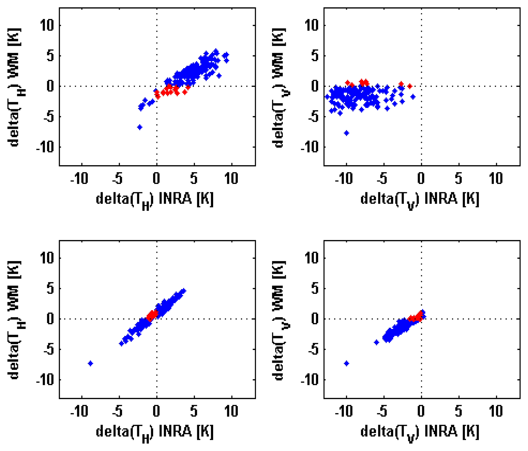
Figure 8 compares for Ka band, the values of ΔT_H achieved by using the INRA model with those obtained with the WM model. The purpose is to show that situations which may be critical for our results, in which the relief causes an overestimation of T_H using one model and an underprediction adopting the other, occur for only few cases (red points in Figure 8). It is worth noting that although for s=0.89 cm the correlation between ΔT_V's is small, the percentage of red points is 5% only. The maximum value of this percentage is 12% (s=0.89 cm, H polarization). We can therefore conclude this discussion on Ka band affirming that, despite the different sensitivities to the observation angle predicted by WM and INRA models, the results that we have achieved can be considered fairly general. What changes is only the magnitude of under- or overestimation, which is model dependent, as expected.

4. Conclusions

A simulation study aiming at quantifying the effects of changes in local observation angle on satellite microwave radiometric observations of a mountainous scene has been presented. A conically-scanning spaceborne radiometer similar to AMSR-E has been assumed. C and X bands, not affected by the atmosphere, as well as Ka band have been analyzed. Only the surface emissivity has been considered in this study that complements the investigation carried out in [2], which mainly concerned the scattered component of the upwelling signal. Our results should therefore be combined with those achieved in [2].

We have found that the changes tend to decrease the upward emissivity towards the sensor. This decrease is contrasted, for horizontal polarization and amplified, for vertical polarization, by the rotation of the plane of linear polarization. Accounting for the beam weighting performed by the radiometer antenna too, we have found that the brightness temperature at vertical polarization and the polarization index are underestimated with respect to the measurements over a flat terrain. The opposite generally occurs for horizontal polarization, although, at Ka band, we have found some situations in which the average observation angle within a radiometric pixel θ_m is very large, so that the effect of the change of the local observation angle prevails on those due to rotation of the polarization plane and beam weighting. To evaluate how these differences affect the retrieval of a bio-geophysical parameter a simple exercise, consisting of the inversion of the forward model to retrieve soil moisture, has been accomplished for C band. A general underestimation of this parameter has been found.

References and Notes

1. Dobson, M. C.; Ulaby, F. T.; Hallikainen, M. T.; El-Rayes, M. Microwave dielectric behavior of wet soil - Part II: Dielectric mixing models. IEEE Trans. Geosci. Rem. Sens. 1985, GE-23, 35–46. [Google Scholar]
2. Mätzler, C.; Standley, A. Technical note: relief effects for passive microwave remote sensing. Int. J. Rem. Sens. 2000, 21, 2403–2412. [Google Scholar]
3. Kerr, Y.H.; Secherre, F.; Lastenet, J.; Wigneron, J.P. SMOS: analysis of perturbing effects over land surfaces. Proc. IEEE/IGARSS 2003, 2, 908–910. [Google Scholar]
4. Talone, M.; Camps, A.; Monerris, A.; Vall-Ilossera, M.; Ferrazzoli, P.; Piles, M. Surface Topography and Mixed-Pixel Effects on the Simulated L-Band Brightness Temperatures. IEEE Trans. Geosci. Rem. Sens. 2007, 45, 1996–2003. [Google Scholar]
5. Wegmüller, U.; Mätzler, C. Rough bare soil reflectivity model. IEEE Trans. Geosci. Remote Sens. 1999, 37, 1391–1395. [Google Scholar]
6. Prigent, C.; Wigneron, J. P.; Rossow, W. B.; Pardo-Carrion, J. R. Frequency and Angular Variations of Land Surface Microwave Emissivities: Can We Estimate SSM/T and AMSU Emissivities from SSM/I Emissivities. IEEE Trans. Geosci. Rem. Sens. 2000, 38, 2373–2386. [Google Scholar]
7. Kawanishi, T.; Sezai, T.; Ito, Y.; Imaoka, K.; Takeshima, T.; Ishido, Y.; Shibata, A.; Miura, M.; Inahata, H.; Spencer, R. W. The advanced microwave scanning radiometer for the earth observing system (AMSR-E), NASDA's Contribution to the EOS for global energy and water cycle studies. IEEE Trans. Geosci. Remote Sens. 2003, 41, 184–194. [Google Scholar]
8. Kerr, Y. H.; Njoku, E. G. A semi empirical model f or interpreting microwave emission from semiarid land surfaces as seen from space. IEEE Trans. Geosci. Remote Sens. 1990, 28, 384–393. [Google Scholar]
9. Calvet, J.-C.; Wigneron, J.-P.; Chanzy, A.; Raju, S.; Laguerre, L. Microwave dielectric properties of a silt-loam at high frequencies. IEEE Trans. Geosci. Rem. Sens. 1995, 33, 634–642. [Google Scholar]
10. Lyzenga, D.R. Comparison of WindSat Brightness Temperatures With Two-Scale Model Predictions. IEEE Trans. Geosci. Rem. Sens. 2006, 44, 560–568. [Google Scholar]
11. Jackson, T.J.; Hurkmans, R.; Hsu, A.; Cosh, M.H. Soil moisture algorithm validation using data from the Advanced Microwave Scanning Radiometer (AMSR-E) in Mongolia. Italian Journal of Remote Sensing 2004, 30/31, 39–52. [Google Scholar]
Figure 1. Emissivity versus observation angle for a bare soil according to the WM model (left panel: s=0.89 cm; central panel: s=1.91 cm) and to the INRA model (right panel, only Ka band). Dotted and solid lines concern V and H polarizations, respectively.
Sensors 08 01459f1
Figure 2. Measurement geometry assumed in the simulation. Upper panel shows the conical scan at 36 GHz. The green ellipses represent the radiometric pixels, θ is the observation angle and R the satellite altitude (scaled for the sake of figure clarity). Lower panel illustrates the observation of a single radiometric pixel in which N elements of the DEM are included. The relief is represented by the local surface normal ni (i=1:N), by the slope angle βi (i=1:N), and by the local observation angle θli (i=1:N). A indicates the area of a DEM element projected on the horizontal plane.
Sensors 08 01459f2
Figure 3. Histograms (Normalized Occurrences: NO) of the local observation angle (upper panel) and of the emissivities at 6 GHz (WM model) for H (central panel) and V (bottom panel) polarizations and for a bare surface with s=0.89 cm. In the upper panel, the local observation angles greater than 90° have been represented by the bar at −10° for the sake of plot clarity.
Sensors 08 01459f3
Figure 4. Trend of TH (left panel), TV (central panel) and PI multiplied by 103 (right panel) versus average observation angle (θm) at 6 GHz (WM model) for a bare surface with s=0.89 cm.
Sensors 08 01459f4
Figure 5. Histograms (Normalized Occurences: NO) of the retrieved SMC computed by inverting the forward model assuming a constant observation angle of 55°.
Sensors 08 01459f5
Figure 6. Trend of TH (left panel), TV (central panel) and PI multiplied by 103 (right panel) versus average observation angle (θm) at 36 GHz (WM model) for a bare surface with s=0.89 cm.
Sensors 08 01459f6
Figure 7. Same of Figure 6 (36 GHz, s=0.89 cm), but for the INRA model.
Sensors 08 01459f7
Figure 8. Comparison between the values of ΔTH obtained, for Ka band, with the two emissivity models. Upper and lower panels concern s=0.89 cm and s=1.91 cm, respectively. Left and right panel concern H and V polarizations, respectively.
Sensors 08 01459f8